Formation and Persistence of Spatiotemporal Turing Patterns

Abstract.

This article is concerned with the stability and long-time dynamics of structures arising from a structureless state. The paradigm is suggested by developmental biology, where morphogenesis is thought to result from a competition between chemical reactions and spatial diffusion. A system of two reaction–diffusion equations for the concentrations of two morphogens is reduced to a finite system of ordinary differential equations. The stability of bifurcated solutions of this system is analyzed, and the long-time asymptotic behavior of the bifurcated solutions is established rigorously. The Schnakenberg and Gierer–Meinhardt equations are discussed as examples.

1. Introduction

Morphogenesis—that is, the development and formation of tissues and organs—is one of the main mysteries in living organisms. How does structure emerge from a structureless state without the apparent action of an external organizing force? A major factor seems to be the competition between chemical reactions and spatial diffusion of substances called morphogens, which are present in the cells. The idea goes back to the pioneering work of Turing in 1952 [24], who noted that diffusion in a mixture of chemically reacting morphogens can cause instability of a spatially uniform steady state and lead to the formation of spatial patterns; see the article by Cross and Hohenberg [3] and the recent text by Hoyle [8] for a comprehensive overview of the theory of pattern formation and Turing analysis.

Turing’s analysis, which is essentially a linear eigenvalue analysis, has been a basic tool in the study of nonlinear reaction–diffusion systems; in fact, it has provided insight into the behavior of nonlinear systems as well, since the latter can often be approximated, at least for brief lengths of time, by linearized systems. But as time evolves, the nonlinear structure takes over, and other tools are needed to study the long-time behavior. In certain cases, where the existence of invariant regions for reaction–diffusion systems can be established, the solution of a nonlinear system remains bounded [22]; however, even in these cases it is not known rigorously whether the patterns persist in the long run, even though the idea is supported by many numerical simulations.

The mathematical literature contains many instances of weakly nonlinear stability analyses for reaction–diffusion systems. An early reference is [6], where a center-manifold approach is used; other, more recent references are [26, 27]. Sometimes, special techniques have been applied to the study of Turing patterns in different regimes. For example, Ref. [9] deals with the stability of symmetric $N$-peaked steady states for systems where the inhibitor diffuses much more rapidly than the activator. We also mention Refs. [1, 18], which deal with the Schnakenberg model on a two-dimensional square domain, where spatially varying diffusion coefficients cause the removal of the degeneracy of the Turing bifurcation.

Weakly nonlinear stability analyses can be justified rigorously on the basis of modulation theory and a Ginzburg–Landau approximation; see, for example, Refs. [2, 4, 20, 21, 25]. Murray’s monograph [14] gives applications to biological systems such as animal coat patterns.

The purpose of the present work is to investigate the nonlinear stability and persistence of spatiotemporal patterns on bounded domains. The investigation is based on recent results of Ma and Wang [11] on attractor bifurcation for nonlinear equations. The attractor bifurcation theorem (see the Appendix, Section A.1) sums up the basic features of a stability-breaking bifurcation. Starting from the original partial differential equation, it identifies and characterizes the local basins of attraction based on the multiplicity of the eigenvalues near a bifurcation point. Thus, the attractor bifurcation theorem gives the complete picture, rather than the caricature given by the amplitude equations.

A second essential feature of the present investigation is a center-manifold reduction to reduce the partial differential equation to a finite-dimensional dynamical system. The reduction requires the computation of the center-manifold function and the interaction of the higher-order eigenfunctions with the eigenspace belonging to the leading eigenvalues. Such a reduction is inherently difficult, and for this reason one usually resorts to a generic form of the reduced equation which is somewhat detached from the original. On the other hand, a center-manifold reduction offers a practical way to find the structure of the local attractors of the original partial differential equation. These attractors completely describe the local transitions, and their basins of attraction define the long-time dynamics associated with the transitions. Since these are exactly the features of interest, we have taken this approach and focused much of our efforts on the center-manifold reduction. As a result, we are able to characterize the types of transitions in terms of explicitly computable parameters which depend only on the domain and the values of the physical parameters of the system under consideration.

We prove that spatiotemporal patterns in reaction–diffusion systems of the attractor–inhibitor type can arise as the result of a supercritical (pitchfork) or subcritical bifurcation. The former results in a continuous transition, the latter in a discontinuous transition. In the case of diffusion on a (bounded) interval or on a rectangular (non-square) domain, we prove that the attractor consists of two points, each with its basin of attraction (Theorem 4.1, Fig. 2). In the case of diffusion on a (bounded) square, the phase diagram after bifurcation consists of eight steady-state solutions and their connecting heteroclinic orbits (Theorem 5.1, Fig. 3). The conditions for the stability of these bifurcated steady states and the heteroclinic orbits are explicit; they can be verified in terms of eigenvalues and eigenvectors. In the framework of classical bifurcation theory, such an explicit characterization is very difficult, if not impossible, and the existence of heteroclinic orbits for a partial differential equation is often hard to prove.

Although the focus in this article is on activator–inhibitor systems, the analysis is quite general and applies, for example, to systems consisting of a self-amplifying activator and a depleted substrate.

Following is an outline of the paper. In Section 2, we formulate the reaction–diffusion problem for an activator–inhibitor mixture and rewrite it as an evolution equation in a function space. In Section 3, we study the exchange of stability, which is crucial for the stability and bifurcation analysis. The results of the bifurcation analysis are summarized for the one-dimensional case in Section 4 and the two-dimensional case in Section 5. In Section 6, we illustrate the theoretical results on two examples, namely the Schnakenberg equation and the Gierer–Meinhardt equations. Section 7 summarizes our conclusions. Appendix A contains a brief summary of the attractor bifurcation theory from Ref. [11] and the reduction method introduced in Ref. [12].

2. Statement of the Problem

Consider a mixture of two chemical species which simultaneously react and diffuse; one of the species is an activator, the other an inhibitor of the chemical reaction. Their respective concentrations $U$ and $V$ satisfy a system of coupled nonlinear reaction–diffusion equations,

(2.1) $$\begin{split}U_{t}&=f(U,V)+d_{1}\Delta U,\\ V_{t}&=g(U,V)+d_{2}\Delta V,\end{split}$$

subject to no-flux boundary conditions and given initial conditions. The functions $f$ and $g$, which describe the kinetics of the chemical reaction, are generally nonlinear functions of the arguments. The diffusion coefficients $d_{1}$ and $d_{2}$ are constant and positive.

We assume that the system of Eqs. (2.1) admits a uniform steady-state solution which is positive throughout the domain. That is, there exist constants $\bar{u}>0$ and $\bar{v}>0$ such that

(2.2) $$f(\bar{u},\bar{v})=0,\quad g(\bar{u},\bar{v})=0.$$

We are interested in solutions that bifurcate from this equilibrium solution and, in particular, in their long-term dynamics, under the assumption that the equilibrium solution (2.2) is stable in the absence of diffusion.

For the bifurcation analysis, it is convenient to rescale time and space and rewrite the system (2.1) in the form

(2.3) $$\begin{split}U_{t}&=\gamma f(U,V)+\Delta U,\\ V_{t}&=\gamma g(U,V)+d\Delta V,\end{split}$$

where $\gamma=1/d_{1}$ and $d=d_{2}/d_{1}$. Thus, $\gamma$ is a measure of the ratio of the characteristic times for diffusion and chemical reaction, and $d$ is the ratio of the diffusion coefficients of the two species. The above equations are satisfied on an open bounded domain, say $\Omega\subset\mathbf{R}^{n}$ ($n=1,2$), while $U$ and $V$ satisfy Neumann (no-flux) boundary conditions on the boundary $\partial\Omega$ of $\Omega$.

2.1. Bifurcation Problem

Let

(2.4) $$U=\bar{u}+u,\quad V=\bar{v}+v.$$

Since $\bar{u}$ and $\bar{v}$ satisfy the identities (2.2), we have

(2.5) $$\begin{split}f(U,V)&=f_{u}(\bar{u},\bar{v})u+f_{v}(\bar{u},\bar{v})v+f_{1}(u,v),\\ g(U,V)&=g_{u}(\bar{u},\bar{v})u+g_{v}(\bar{u},\bar{v})v+g_{1}(u,v),\end{split}$$

where $f_{1}$ and $g_{1}$ incorporate the higher-order terms in the Taylor expansions. The functions $u$ and $v$ satisfy the equations

(2.6) $$\begin{split}u_{t}&=\Delta u+\gamma(f_{u}(\bar{u},\bar{v})u+f_{v}(\bar{u},\bar{v})v)+\gamma f_{1}(u,v),\\ v_{t}&=d\Delta v+\gamma(g_{u}(\bar{u},\bar{v})u+g_{v}(\bar{u},\bar{v})v)+\gamma g_{1}(u,v).\end{split}$$

Henceforth we omit the arguments $(\bar{u},\bar{v})$ and use the abbreviations $f_{u}$ for $f_{u}(\bar{u},\bar{v})$, et cetera.

Since the variables $U$ and $V$ are associated with the activator and the inhibitor, respectively, of the chemical reaction, we have the inequalities

(2.7) $$f_{u}>0,\quad g_{v}<0.$$

The equilibrium solution (2.2) is stable in the absence of diffusion, so we also have the inequalities

(2.8) $$f_{u}g_{v}-f_{v}g_{u}>0,\quad f_{u}+g_{v}<0.$$

The first inequality in (2.8), together with the inequalities (2.7), implies that $f_{v}g_{u}<0$.

The problem as stated has two parameters, $\gamma$ and $d$. We represent the ordered pair by a single symbol, $\lambda=(\gamma,d)$, and consider $\lambda$ as the bifurcation parameter. The bifurcation is from the trivial solution, $(u,v)=(0,0)$.

2.2. Abstract Evolution Equation

The system of Eqs. (2.6) defines an abstract evolution equation for a vector-valued function $w:[0,\infty)\to H=(L^{2}(\Omega))^{2}$,

(2.9) $$\frac{dw}{dt}=L_{\lambda}w+G_{\lambda}(w),\,t>0;\quad w(t)=\left(\begin{array}[]{c}u(\cdot\,,t)\\ v(\cdot\,,t)\end{array}\right).$$

Here, $L_{\lambda}$ a linear operator in $H$ of the form

(2.10) $$L_{\lambda}=-AD+\gamma B,$$

where $A:\mathrm{dom}(A)\to H$ is given by the expression

(2.11) $$A=-\Delta I=\left(\begin{array}[]{cc}-\Delta&0\\ 0&-\Delta\end{array}\right),$$

on $\mathrm{dom}(A)=H_{1}=\{w\in(H^{2}(\Omega))^{2}:n\cdot\nabla w=0\mathrm{~{}on~{}}\partial\Omega\}$, and $B:H\to H$ and $D:H\to H$ are represented by the constant matrices

(2.12) $$B=\left(\begin{array}[]{cc}f_{u}&f_{v}\\ g_{u}&g_{v}\end{array}\right),\quad D=\left(\begin{array}[]{cc}1&0\\ 0&d\end{array}\right).$$

In Eq. (2.11), $\Delta$ denotes the Laplacian, $H^{2}(\Omega)$ is the usual Sobolev space, and the gradient on the boundary $\partial\Omega$ of $\Omega$ is taken component-wise.

The nonlinear operator $G_{\lambda}:H\to H$ is given by

(2.13) $$G_{\lambda}:w=\left(\begin{array}[]{c}u\\ v\end{array}\right)\mapsto\gamma\left(\begin{array}[]{c}f_{1}(u,v)\\ g_{1}(u,v)\end{array}\right),$$

Without loss of generality, we assume that $G_{\lambda}$ can be written as the sum of symmetric multilinear forms,

(2.14) $$G_{\lambda}(w)=\sum_{k=2}^{\infty}G_{\lambda,k}(w,\ldots\,,w),$$

where $G_{k}$ is a symmetric $k$-linear form ($k=2,3,\ldots$). When the $k$ arguments of $G_{k}$ coincide, we write $G_{k}$ with a single argument, $G_{k}(w)=G_{k}(w,\ldots\,,w)$.

The abstract evolution equation (2.9) belongs to a class of equations analyzed in detail in Ref. [11]; the relevant results are summarized for reference purposes in the Appendix, Section A.1.

3. Exchange of Stability

The inequalities (2.8) imply that

(3.1) $$\mathrm{det}(B)>0,\quad\mathrm{tr}(B)<0.$$

Under these conditions, diffusion has a destabilizing effect: At some critical value $\lambda_{0}$ of $\lambda$, an exchange of stability occurs and the solution of Eq. (2.9) bifurcates from the trivial solution.

3.1. Eigenvalues and Eigenvectors of $L_{\lambda}$ and $L^{*}_{\lambda}$

The negative Laplacian $-\Delta$ on a bounded domain $\Omega\in\mathbf{R}^{n}$ with Neumann boundary conditions is selfadjoint and positive in $L^{2}(\Omega)$. Its spectrum is discrete, consisting of eigenvalues $\rho_{k}$ with corresponding eigenvectors $\varphi_{k}$,

(3.2) $$-\Delta\varphi_{k}=\rho_{k}\varphi_{k},\quad k=1,2,\ldots\,,$$

We assume that the eigenvalues are ordered, $0<\rho_{1}\leq\rho_{2}\leq\cdots\,$, and that the eigenvectors $\{\varphi_{k}\}_{k}$ form a basis in $L^{2}(\Omega)$.

It follows from the definition (2.11) that $A$ is selfadjoint and positive in $H$; its spectrum is also discrete, consisting of the same eigenvalues $\rho_{k}$ and the eigenvectors $\varphi_{k}$ once repeated. The operator $L_{\lambda}$ reduces via projection to its components on the linear span of each eigenvector of $A$. Let $E_{k}$ be the component of $L_{\lambda}$ in the eigenspace associated with the eigenvalue $\rho_{k}$,

(3.3) $$E_{k}(\lambda)=-\rho_{k}D+\gamma B,\quad k=1,2,\ldots\,.$$

The determinant and trace of $E_{k}(\lambda)$ are

(3.4) $$\begin{split}\mathrm{det}(E_{k}(\lambda))&=\gamma^{2}\mathrm{det}(B)+\gamma\rho_{k}|g_{v}|-\rho_{k}d(\gamma f_{u}-\rho_{k}),\\ \mathrm{tr}(E_{k}(\lambda))&=\gamma\,\mathrm{tr}(B)-\rho_{k}(1+d).\end{split}$$

Note that $\mathrm{tr}(E_{k}(\lambda))$ is negative everywhere in the first quadrant and becomes more negative as $k$ increases.

The eigenvalues of $E_{k}(\lambda)$ come in pairs,

(3.5) $$\beta_{ki}(\lambda)=\textstyle{\frac{1}{2}}\left(\mathrm{tr}(E_{k}(\lambda))\pm\left((\mathrm{tr}(E_{k}(\lambda))^{2}-4\,\mathrm{det}(E_{k}(\lambda))\right)^{1/2}\right),\quad i=1,2.$$

They are either complex conjugate, with $\Re\beta_{k1}=\Re\beta_{k2}<0$, or they are both real, with $\beta_{k1}+\beta_{k2}<0$. We identify $\beta_{k1}$ with the upper ($+$) sign and $\beta_{k2}$ with the lower ($-$) sign, so $\Re\beta_{k2}\leq\Re\beta_{k1}$.

The eigenvector corresponding to the eigenvalue $\beta_{ki}$ of $L_{\lambda}$ is

(3.6) $$w_{ki}=\left(\begin{array}[]{c}-\gamma f_{v}\varphi_{k}\\ (\gamma f_{u}-\rho_{k}-\beta_{ki})\varphi_{k}\end{array}\right).$$

The eigenvectors $w_{k1}$ and $w_{k2}$ are linearly independent as long as $\beta_{k1}\neq\beta_{k2}$. The set of eigenvectors $\{w_{ki}\}_{k,i}$ forms a basis for $H$.

Note that $B$ is not symmetric; its adjoint $B^{*}$ is the transpose $B^{\prime}$ of $B$. Hence, the adjoint of $L_{\lambda}$ is $L^{*}_{\lambda}=-AD+\gamma B^{\prime}$, and the adjoint of $E_{k}(\lambda)$ is $E_{k}^{*}(\lambda)=-\rho_{k}D+\gamma B^{\prime}$. The eigenvalues of $E_{k}^{*}(\lambda)$ are $\bar{\beta}_{ki}$, $i=1,2$, the complex conjugates of the eigenvalues $\beta_{ki}$ of $E_{k}(\lambda)$ given in Eq. (3.5). Since the latter are either complex conjugate or real, the eigenvalues of $L_{\lambda}$ and $L_{\lambda}^{*}$ coincide. The eigenvector corresponding to the eigenvalue $\bar{\beta}_{ki}$ of $L_{\lambda}^{*}(\lambda)$ is

(3.7) $$w^{*}_{ki}=\left(\begin{array}[]{c}-\gamma g_{u}\varphi_{k}\\ (\gamma f_{u}-\rho_{k}-\bar{\beta}_{ki})\varphi_{k}\end{array}\right).$$

3.2. Exchange of Stability

The equation $\mathrm{det}(E_{k}(\lambda))=0$ defines a curve $\Lambda_{k}$ in the $(\gamma,d)$-plane,

(3.8) $$\Lambda_{k}=\{(\gamma,d):\mathrm{det}(E_{k}(\lambda))=0\}=\{(\gamma,d):d=d_{k}(\gamma)\},\quad k=1,2,\ldots,$$

where

(3.9) $$d_{k}(\gamma)=\frac{\gamma^{2}\mathrm{det}(B)+\gamma\rho_{k}|g_{v}|}{\rho_{k}(\gamma f_{u}-\rho_{k})}.$$

The expression for $d_{k}$ can be recast in the form

(3.10) $$d_{k}(\gamma)-d^{(s)}=\frac{\rho_{k}|f_{v}g_{u}|}{f_{u}^{3}}(\gamma-\gamma_{k}^{(s)})^{-1}+\frac{\mathrm{det}(B)}{\rho_{k}f_{u}}(\gamma-\gamma_{k}^{(s)})^{-1},$$

where $\gamma_{k}^{(s)}=\rho_{k}/f_{u}$ and $d^{(s)}=(\mathrm{det}(B)+|f_{v}g_{u}|)/f_{u}^{2}$. This expression shows that (i)  $\Lambda_{k}$ is symmetric with respect to the point $(\gamma_{k}^{(s)},d^{(s)})$ (ii)  $\Lambda_{k}$ has a vertical asymptote at $\gamma=\rho_{k}/f_{u}$; and (iii)  $\Lambda_{k}$ has an oblique asymptote with slope $\mathrm{det}(B)/(\rho_{k}f_{u})$. The symmetry point $(\gamma_{k}^{(s)},d^{(s)})$ is located in the first quadrant of the $(\gamma,d)$-plane; $\gamma_{k}^{(s)}$ increases as $k$ increases, $d^{(s)}$ is independent of $k$. The vertical asymptote is in the right-half of the $(\gamma,d)$-plane, shifting to the right as $k$ increases. The slope of the oblique asymptote is positive, decreasing to zero as $k$ increases. Therefore, each curve $\Lambda_{k}$ has a branch in the positive quadrant of the $(\gamma,d)$-plane. The positive branches of the curves $\Lambda_{1}$ and $\Lambda_{2}$ are sketched in Fig. 1.

Figure 1. Positive branches of $\Lambda_{1}$ and $\Lambda_{2}$.

The curve $\Lambda_{k}$ separates the region where $\mathrm{det}(E_{k}(\lambda))>0$ (below the curve) from the region where $\mathrm{det}(E_{k}(\lambda))<0$ (above the curve). We focus on the region below the curve $\Lambda_{2}$, bounded on the left by the first vertical asymptote at $\gamma=\rho_{1}/f_{u}$ and on the right by $\gamma=\gamma_{1}$, where the curves $\Lambda_{1}$ and $\Lambda_{2}$ cross (see Fig. 1). The curve $\Lambda_{1}$ separates this region into two subregions,

(3.11) $$\begin{split}R_{1}&=\{\lambda=(\gamma,d):\rho_{1}/f_{u}<\gamma<\gamma_{1},\,0<d<d_{1}(\gamma)\},\\ R_{2}&=\{\lambda=(\gamma,d):\rho_{1}/f_{u}<\gamma<\gamma_{1},\,d_{1}(\gamma)<d<d_{2}(\gamma)\}.\end{split}$$

These regions are indicated in Fig.1.

Lemma 3.1.

The eigenvalues $\beta_{1i}$ ($i=1,2$) of $L_{\lambda}$ satisfy the inequalities

(3.12) $$\begin{array}[]{ll}\Re\beta_{11}(\lambda)<0,\,\Re\beta_{12}(\lambda)<0&\text{~{}if~{}}\lambda\in R_{1},\\ \beta_{11}(\lambda)=0,\,\beta_{12}(\lambda)<0&\text{~{}if~{}}\lambda\in\Lambda_{1},\\ \beta_{11}(\lambda)>0,\,\beta_{12}(\lambda)<0&\text{~{}if~{}}\lambda\in R_{2}.\\ \end{array}$$

Furthermore, for $k=2,3,\ldots\,$,

(3.13) $$\Re\beta_{k1}(\lambda)<0,\,\Re\beta_{k2}(\lambda)<0\,\text{~{}if~{}}\lambda\in\Lambda_{1}.$$

Proof.

In $R_{1}$, we have $\mathrm{tr}(E_{1}(\lambda))<0$ and $\mathrm{det}(E_{1}(\lambda)>0$, so $\beta_{11}(\lambda)$ and $\beta_{12}(\lambda)$ are either complex conjugate with a negative real part, or they are both real and negative. On $\Lambda_{1}$, the leading eigenvalue $\beta_{11}(\lambda)$ is zero. Since $\mathrm{tr}(E_{1}(\lambda))<0$, it must be the case that $\beta_{12}(\lambda)$ is real and negative. In $R_{2}$, we have $\mathrm{tr}(E_{1}(\lambda))<0$ and $\mathrm{det}(E_{1}(\lambda)<0$, so $\beta_{11}(\lambda)$ and $\beta_{12}(\lambda)$ are both real, and they have opposite signs.

On $\Lambda_{1}$, $\mathrm{det}(E_{2}(\lambda))>0$. Since $\mathrm{det}(E_{k}(\lambda))$ increases with $k$, it follows that $\mathrm{det}(E_{k}(\lambda))>0$ for $k=2,3,\ldots$. Also, $\mathrm{tr}(E_{k}(\lambda))<0$. Hence, either $\beta_{k1}(\lambda)$ and $\beta_{k2}(\lambda)$ are complex conjugate with a negative real part, or they are both real and negative. ∎

The lemma implies that all eigenmodes are stable as long as $\lambda$ is below the curve $\Lambda_{1}$. However, as soon as $\lambda$ crosses the “critical curve” $\Lambda_{1}$, the first unstable eigenmode appears and an exchange of stability occurs.

4. Bifurcation Analysis – One-dimensional Domain

We first consider the bifurcation problem (2.9) on a one-dimensional domain $\Omega=(0,\ell)$. We reduce Eq. (2.9) to its center-manifold representation near a point $\lambda_{0}$ on the critical curve $\Lambda_{1}$, as proposed in Ref. [12] and sketched in the Appendix, Section A.2.

The eigenvalues and eigenvectors of the negative Laplacian subject to Neumann boundary conditions (see Eq. (3.2)) are

$$\rho_{k}=k^{2}(\pi/\ell)^{2},\quad\varphi_{k}(x)=\cos(k(\pi/\ell)x),\,x\in\Omega;\qquad k=1,2,\ldots.$$

The linear operator $L_{\lambda}$ decomposes into its components

(4.1) $$E_{k}(\lambda)=-k^{2}(\pi/\ell)^{2}D+\gamma B,\quad k=1,2,\ldots\,,$$

with

(4.2) $$\begin{split}\mathrm{det}(E_{k}(\lambda))&=\gamma^{2}\mathrm{det}(B)+\gamma|g_{v}|k^{2}(\pi/\ell)^{2}-dk^{2}(\pi/\ell)^{2}(\gamma f_{u}-k^{2}(\pi/\ell)^{2}),\\ \mathrm{tr}(E_{k}(\lambda))&=\gamma\mathrm{tr}(B)-(1+d)k^{2}(\pi/\ell)^{2}.\end{split}$$

Each $E_{k}$ contributes two eigenvalues, $\beta_{k1}$ and $\beta_{k2}$, to the spectrum of $L_{\lambda}$; the expressions for $\beta_{ki}$ ($i=1,2$) in terms of $\mathrm{det}(E_{k}(\lambda))$ and $\mathrm{tr}(E_{k}(\lambda))$ are given in Eq. (3.5). The eigenvalues of the adjoint $L_{\lambda}^{*}$ are the complex conjugates, $\bar{\beta}_{k1}$ and $\bar{\beta}_{k2}$. The eigenvectors of $L_{\lambda}$ and $L_{\lambda}^{*}$ corresponding to the eigenvalues $\beta_{ki}$ and $\bar{\beta}_{ki}$ are

(4.3) $$w_{ki}=\left(\begin{array}[]{c}-\gamma f_{v}\cos(k(\pi/\ell)x)\\ (\gamma f_{u}-k^{2}(\pi/\ell)^{2}-\beta_{ki})\cos(k(\pi/\ell)x)\end{array}\right)$$

and

(4.4) $$w_{ki}^{*}=\left(\begin{array}[]{c}-\gamma g_{u}\cos(k(\pi/\ell)x)\\ (\gamma f_{u}-k^{2}(\pi/\ell)^{2}-\bar{\beta}_{ki})\cos(k(\pi/\ell)x)\end{array}\right),$$

respectively.

4.1. Center-manifold Reduction

We are interested in solutions of Eq. (2.9) near a point $\lambda_{0}$ on the critical curve $\Lambda_{1}$. In the region $R_{1}$, just below $\Lambda_{1}$, both eigenvalues $\beta_{11}$ and $\beta_{12}$ are real, with $\beta_{12}<\beta_{11}<0$. As $\lambda$ approaches $\lambda_{0}$, the leading eigenvalue $\beta_{11}$ increases and, as $\lambda$ transits into $R_{2}$, $\beta_{11}$ passes through 0 and becomes positive. Thus, the first exchange of stability occurs.

Lemma 4.1.

Near the critical curve $\Lambda_{1}$, the solution of Eq. (2.9) can be expressed in the form

(4.5) $$w=y_{11}w_{11}+z,\quad z=y_{12}w_{12}+\sum_{k=2}^{\infty}\sum_{i=1,2}y_{ki}w_{ki},$$

where the coefficient $y_{11}$ of the leading term satisfies the reduced bifurcation equation,

(4.6) $$\frac{dy_{11}}{dt}=\beta_{11}y_{11}+\alpha y_{11}^{3}+o(|y_{11}|^{3}).$$

The coefficient $\alpha\equiv\alpha(\lambda)$ are given explicitly in terms of the eigenfunctions of $L_{\lambda}$ and $L_{\lambda}^{*}$,

(4.7) $$\alpha(\lambda)=\alpha_{2}(\lambda)+\alpha_{3}(\lambda),$$

where

$$\alpha_{2}(\lambda) =\frac{2}{<w_{11},w_{11}^{*}>}\sum_{i=1,2}\frac{<G_{2}(w_{11},w_{2i}),w_{11}^{*}><G_{2}(w_{11}),w_{2i}^{*}>}{(2\beta_{11}-\beta_{2i})<w_{2i},w_{2i}^{*}>},$$

$$\alpha_{3}(\lambda) =\frac{1}{<w_{11},w_{11}^{*}>}<G_{3}(w_{11}),w_{11}^{*}>.$$

Here, $<\cdot\,,\cdot>$ denotes the inner product in $H$. (The subscript $\lambda$ on the $k$-linear forms has been omitted.)

Proof.

We look for a solution $w$ of Eq. (2.9) of the form (4.5). In the space spanned by the eigenvector $w_{11}$, Eq. (2.9) reduces to

(4.8) $$\begin{split}<w_{11},w_{11}^{*}>\frac{dy_{11}}{dt}&=\ <L_{\lambda}w,w_{11}^{*}>\ +\ <G_{\lambda}(w),w_{11}^{*}>\\ &=\ \beta_{11}<w_{11},w_{11}^{*}>y_{11}\ +\ \sum_{k=2}^{\infty}<G_{k}(w),w_{11}^{*}>.\end{split}$$

To evaluate the contributions from the various terms in the sum, we use the asymptotic expression for the center-manifold function near $\lambda_{0}$ given in the Appendix (Section A.2), Theorem A.2,

(4.9) $$y_{ki}=\Phi^{\lambda}_{ki}(y_{11})=\frac{<G_{2}(w_{11}),w_{ki}^{*}>y_{11}^{2}}{(2\beta_{11}-\beta_{ki})<w_{ki},w_{ki}^{*}>}+o(|y_{11}|^{2}),\quad k=2,3,\ldots\,.$$

The contribution from the bilinear form ($k=2$) is

$$<G_{2}(w),w_{11}^{*}> =\ <G_{2}(y_{11}w_{11}+z),w_{11}^{*}>$$

$$=\ <G_{2}(w_{11}),w_{11}^{*}>y_{11}^{2}$$

$$\hskip 20.00003pt+\ 2<G_{2}(w_{11},z),w_{11}^{*}>y_{11}+<G_{2}(z),w_{11}^{*}>.$$

The first term in the right member vanishes, because

$$<G_{2}(w_{11}),w_{11}^{*}>\ =0.$$

The second and third term can be evaluated by means of the asymptotic expression (4.9) for the center manifold,

$$<G_{2}(w_{11},z),w_{11}^{*}> =\sum_{i=1,2}<G_{2}(w_{11},w_{2i}),w_{11}^{*}>y_{2i}+\ o(|y_{11}|^{2})$$

$$=\ \textstyle{\frac{1}{2}}\alpha_{2}<w_{11},w_{11}^{*}>y_{11}^{2}+o(|y_{11}|^{2}),$$

$$<G_{2}(z),w_{11}^{*}> =o(|y_{11}|^{3}),$$

where $\alpha_{2}$ is defined in Eq. (4.7). Putting it all together, we obtain the asymptotic result

(4.10) $$<G_{2}(w),w_{11}^{*}>\ =\ \alpha_{2}<w_{11},w_{11}^{*}>y_{11}^{3}+o(|y_{11}|^{3}).$$

The contribution from the trilinear form ($k=3$) is

(4.11) $$\begin{split}<G_{3}(w),w_{11}^{*}>&=\ <G_{3}(w_{11}),w_{11}^{*}>y_{11}^{3}+o(|y_{11}|^{3})\\ &=\ \alpha_{3}<w_{11},w_{11}^{*}>y_{11}^{3}+o(|y_{11}|^{3}),\end{split}$$

where $\alpha_{3}$ is defined in Eq. (4.7). The higher-order forms contribute only terms of $o(|y_{11}|^{3})$. ∎

4.2. Structure of the Bifurcated Attractor

The results of the bifurcation analysis for one-dimensional spatial domains are summarized in the following theorem.

Theorem 4.1.

$\Omega=(0,\ell)$.

• If $\alpha(\lambda_{0})<0$, then the following statements are true:

  1. $w=0$ is a locally asymptotically stable equilibrium point of Eq. (2.9) for $\lambda\in R_{1}$ or $\lambda\in\Lambda_{1}$.

  2. The solution of Eq. (2.9) bifurcates supercritically from $(\lambda_{0},0)$ to an attractor $\mathcal{A}_{\lambda}$ as $\lambda$ crosses $\Lambda_{1}$ from $R_{1}$ into $R_{2}$.

  3. There exists an open set $U_{\lambda}\subset H$ with $0\in U_{\lambda}$ such that the bifurcated attractor $\mathcal{A}_{\lambda}$ attracts $U_{\lambda}\setminus\Gamma$ in $H$, where $\Gamma$ is the stable manifold of $0$ with codimension $1$.

  4. The attractor $\mathcal{A}_{\lambda}$ consists of two steady-state points, $w_{\lambda}^{+}$ and $w_{\lambda}^{-}$,

     (4.12) $$w_{\lambda}^{\pm}={\pm}(\beta_{11}/|\alpha|)^{1/2}w_{11}+\omega_{\lambda},\quad\lambda\in R_{2},$$

     where $\|\omega_{\lambda}\|_{H}=o(\beta_{11}^{1/2})$.

  5. There exists an $\varepsilon>0$ and two disjoint open sets $U_{\lambda}^{+}$ and $U_{\lambda}^{-}$ in $H$, with $0\in\partial U_{\lambda}^{+}\cap\partial U_{\lambda}^{-}$, such that $w_{\lambda}^{\pm}\in U_{\lambda}^{\pm}$ and $\lim_{t\to\infty}||w(t;w_{0})-w_{\lambda}^{\pm}||_{H}=0$ for any solution $w(t;w_{0})$ of Eq. (2.9) satisfying the initial condition $w(0;w_{0})=w_{0}\in U_{\lambda}^{\pm}$ and any $\lambda$ satisfying the condition $\mathrm{dist}(\lambda_{0},\lambda)<\varepsilon$.

• If $\alpha(\lambda_{0})>0$, then the solution of Eq. (2.9) bifurcates subcritically from $(\lambda_{0},0)$ to exactly two repeller points as $\lambda$ crosses $\Lambda_{1}$ from $R_{2}$ into $R_{1}$.

Proof.

Equation (4.6) shows that, if $\alpha(\lambda_{0})<0$, then $w=0$ is a locally asymptotically stable equilibrium point.

According to the attractor bifurcation theorem (Section A.1, Theorem A.1), the system bifurcates at $(\lambda_{0},0)$ to an attractor $\mathcal{A}_{\lambda}$ as $\lambda$ transits from $R_{1}$ into $R_{2}$.

The structure of the attractor follows from the stationary form of Eq. (4.6),

$$\beta_{11}y_{11}+\alpha y_{11}^{3}+o(|y_{11}|^{3})=0.$$

The number and nature of the solutions of this equation does not change if the terms of $o(|y_{11}|^{3})$ are ignored, provided all solutions are regular at the origin. Thus, if $\alpha<0$, we find two solutions near $y=0$,

(4.13) $$y_{11}=\pm(\beta_{11}/|\alpha|)^{1/2}+o(\beta^{1/2}).$$

The last assertion of the theorem follows by time reversal. ∎

Theorem 4.1 shows that, if $\alpha(\lambda_{0})<0$, the attractor consists of two steady-state points, each with its own basin of attraction. The attractor bifurcation is shown schematically in Fig. 2. From the perspective of pattern formation, the theorem predicts the persistence of two types of patterns that differ only in phase; which of the two patterns is actually realized depends on the initial data.

Figure 2. One-dimensional domain: Supercritical bifurcation to an attractor $\mathcal{A}=\{w^{+},w^{-}\}$.

5. Bifurcation Analysis – Two-dimensional Domains

Next, we consider the bifurcation problem (2.9) on a two-dimensional domain $\Omega=(0,\ell_{1})\times(0,\ell_{2})$.

As in the one-dimensional case, we reduce Eq. (2.9) to its center-manifold representation near a point $\lambda_{0}\in\Lambda_{1}$.

The eigenvalues and eigenvectors of the negative Laplacian subject to Neumann boundary conditions (see Eqs. (4.3) and (4.4)) are

$$\begin{split}\rho_{k_{1}k_{2}}&=k_{1}^{2}(\pi/\ell_{1})^{2}+k_{2}^{2}(\pi/\ell_{2})^{2},\\ \varphi_{k_{1}k_{2}}(x)&=\cos(k_{1}(\pi/\ell_{1})x_{1})\cos(k_{2}(\pi/\ell_{2})x_{2}),\,x=(x_{1},x_{2})\in\Omega.\end{split}$$

Here, $k_{1}$ and $k_{2}$ range over all nonnegative integers such that $|k|=k_{1}+k_{2}=1,2,\ldots$.

The eigenvalues $\beta_{k_{1}k_{2}i}$ ($i=1,2$) and the corresponding eigenvectors of $L_{\lambda}$ are given in Eqs. (3.5) and (3.6), respectively, where $k$ now stands for the ordered pair $(k_{1},k_{2})$.

The dynamics depend on the relative size of $\ell_{1}$ and $\ell_{2}$. On a rectangular (non-square) domain, they are essentially the same as on a one-dimensional domain. For example, if $\ell_{2}<\ell_{1}$, then $\rho_{10}=(\pi/\ell_{1})^{2}$ is the smallest eigenvalue of the negative Laplacian, with corresponding eigenvector $\varphi_{10}=\cos((\pi/\ell_{1})x_{1})$, and the leading eigenvalue of $L_{\lambda}$ is $\beta_{101}$. This eigenvalue is simple, and the corresponding eigenvector is

(5.1) $$w_{101}=\left(\begin{array}[]{c}-\gamma f_{v}\cos((\pi/\ell_{1})x_{1})\\ (\gamma f_{u}-(\pi/\ell_{1})^{2}-\beta_{101})\cos((\pi/\ell_{1})x_{1})\end{array}\right).$$

The center-manifold reduction leads to a one-dimensional dynamical system similar to Eq. (4.6). Lemma 4.1 and Theorem 4.1 apply verbatim if $\beta_{11}$ is replaced by $\beta_{101}$ and $w_{11}$ by $w_{101}$ everywhere.

On the other hand, the dynamics become qualitatively different if the domain is square—that is, if $\ell_{1}=\ell_{2}=\ell$ and $\Omega=(0,\ell)^{2}$. The eigenvalues and eigenvectors of $-\Delta$ on the square are

$$\rho_{k_{1}k_{2}} =(k_{1}^{2}+k_{2}^{2})(\pi/\ell)^{2},$$

$$\varphi_{k_{1}k_{2}}(x) =\cos(k_{1}(\pi/\ell)x_{1})\cos(k_{2}(\pi/\ell)x_{2}),\quad x=(x_{1},x_{2}).$$

Note that $\rho_{k_{1}k_{2}}=\rho_{k_{2}k_{1}}$ for any pair $(k_{1},k_{2})$, so the eigenvalues $\beta_{k_{1}k_{2}i}$ ($i=1,2$) of $L_{\lambda}$ satisfy the same symmetry condition, $\beta_{k_{1}k_{2}i}=\beta_{k_{2}k_{1}i}$. To avoid notational complications, we consider two eigenvalues, even if they coincide because of symmetry, as distinct and associate with each its own eigenvector. Thus, we associate the eigenvector

(5.2) $$w_{k_{1}k_{2}i}=\left(\begin{array}[]{c}-\gamma f_{v}\varphi_{k_{1}k_{2}}\\ (\gamma f_{u}-\rho_{k_{1}k_{2}}-\beta_{k_{1}k_{2}i})\varphi_{k_{1}k_{2}}\end{array}\right)$$

with the eigenvalue $\beta_{k_{1}k_{2}i}$, and the eigenvector

(5.3) $$w_{k_{1}k_{2}i}^{*}=\left(\begin{array}[]{c}-\gamma g_{u}\varphi_{k_{1}k_{2}}\\ (\gamma f_{u}-\rho_{k_{1}k_{2}}-\bar{\beta}_{k_{1}k_{2}i})\varphi_{k_{1}k_{2}}\end{array}\right)$$

with the eigenvalue $\bar{\beta}_{k_{1}k_{2}i}$, whether $k_{1}$ and $k_{2}$ are equal or not.

5.1. Center-manifold Reduction

We are again interested in values of $\lambda$ near the critical curve $\Lambda_{1}$, where the first exchange of stability occurs. The leading eigenvalues are $\beta_{101}$ and $\beta_{011}$. These eigenvalues coincide, but we consider them separately, each with its own eigenvector. The two eigenvalues pass (together) through 0 as $\lambda$ crosses $\Lambda_{1}$ into $R_{2}$ from $R_{1}$, at the value $\lambda=\lambda_{0}$.

Lemma 5.1.

Near the critical curve $\Lambda_{1}$, the solution of Eq. (2.9) can be expressed in the form

(5.4) $$w=y_{1}w_{1}+y_{2}w_{2}+z,\quad z=\sum_{(k_{1},k_{2}):|k|=2,3,\ldots}\sum_{i=1,2}y_{k_{1}k_{2}i}w_{k_{1}k_{2}i},$$

where $w_{1}=w_{101}$ and $w_{2}=w_{011}$. The coefficients $y_{1}$ and $y_{2}$ of the leading terms satisfy a system of equations of the form

(5.5) $$\begin{split}\frac{dy_{1}}{dt}&=\beta_{101}y_{1}+(\alpha y_{1}^{2}+\sigma y_{2}^{2})y_{1}+o(|y|^{3}),\\ \frac{dy_{2}}{dt}&=\beta_{011}y_{2}+(\alpha y_{2}^{2}+\sigma y_{1}^{2})y_{2}+o(|y|^{3}),\end{split}$$

where $\beta_{100}=\beta_{011}$. The coefficients $\alpha\equiv\alpha(\lambda)$ and $\sigma\equiv\sigma(\lambda)$ are given explicitly in terms of the eigenfunctions of $L_{\lambda}$ and $L_{\lambda}^{*}$,

(5.6) $$\alpha(\lambda)=\alpha_{2}(\lambda)+\alpha_{3}(\lambda),$$

where

$$\alpha_{2}(\lambda) =\frac{2}{<w_{1},w_{1}^{*}>}\sum_{i=1,2}\frac{<G_{2}(w_{1},w_{20i}),w^{*}_{1}><G_{2}(w_{1}),w_{20i}^{*}>}{(2\beta_{101}-\beta_{20i})<w_{20i},w_{20i}^{*}>},$$

$$\alpha_{3}(\lambda) =\frac{1}{<w_{1},w_{1}^{*}>}<G_{3}(w_{1}),w_{1}^{*}>,$$

and

(5.7) $$\sigma(\lambda)=\sigma_{2}(\lambda)+\sigma_{3}(\lambda),$$

where

$$\sigma_{2}(\lambda) =\frac{4}{<w_{1},w_{1}^{*}>}\sum_{i=1,2}\frac{<G_{2}(w_{2},w_{11i}),w^{*}_{1}><G_{2}(w_{1},w_{2}),w^{*}_{11}>}{(2\beta_{101}-\beta_{11i})<w_{11i},w_{11i}^{*}>},$$

$$\sigma_{3}(\lambda) =\frac{3}{<w_{1},w_{1}^{*}>}<G_{3}(w_{1},w_{2},w_{2}),w_{1}^{*}>.$$

The asymptotic estimates in Eq. (5.5) are valid as $|y|=\|y_{1}\|+\|y_{2}\|\to 0$.

Proof.

We look for a solution $w$ of Eq. (2.9) of the form (5.4). In the space spanned by the eigenvectors $w_{1}=w_{101}$ and $w_{2}=w_{011}$, Eq. (2.9) reduces to

(5.8) $$\begin{split}<w_{1},w_{1}^{*}>\frac{dy_{1}}{dt}&=\beta_{101}<w_{1},w_{1}^{*}>y_{1}+\sum_{k=2}^{\infty}<G_{k}(w),w_{1}^{*}>,\\ <w_{2},w_{2}^{*}>\frac{dy_{2}}{dt}&=\beta_{011}<w_{2},w_{2}^{*}>y_{2}+\sum_{k=2}^{\infty}<G_{k}(w),w_{2}^{*}>.\end{split}$$

To evaluate the contributions from the various terms in the sums, we again use the asymptotic expression for the center-manifold function near $\lambda_{0}$ given in the Appendix (Section A.2), Theorem A.2,

(5.9) $$\begin{split}y_{k_{1}k_{2}i}&=\Phi^{\lambda}_{k_{1}k_{2}i}(y_{1},y_{2})\\ &=\frac{\sum_{j=1,2}<G_{2}(w_{j}),w_{k_{1}k_{2}i}^{*}>y_{j}^{2}}{(2\beta_{101}-\beta_{k_{1}k_{2}i})<w_{k_{1}k_{2}i},w_{k_{1}k_{2}i}^{*}>}+o(|y|^{2}),\quad k_{1}\not=k_{2},\\ y_{kki}&=\Phi^{\lambda}_{kki}(y_{1},y_{2})=\frac{2<G_{2}(w_{1},w_{2}),w_{kki}^{*}>y_{1}y_{2}}{(2\beta_{101}-\beta_{kki})<w_{kki},w_{kki}^{*}>}+o(|y|^{2}),\end{split}$$

where $|y|^{2}=\|y_{1}\|^{2}+\|y_{2}\|^{2}$.

Consider the first of Eqs. (5.8). The contribution from the bilinear form is

$$<G_{2}(w),w_{1}^{*}> =\ \sum_{i=1,2}<G_{2}(w_{i}),w_{1}^{*}>y_{i}^{2}$$

$$\hskip 20.00003pt+2\sum_{i=1,2}<G_{2}(w_{i},z),w_{1}^{*}>y_{i}+<G_{2}(z),w_{1}^{*}>.$$

The first term in the right member vanishes, because

$$<G_{2}(w_{i}),w_{1}^{*}>\ =0,\quad i=1,2.$$

The last term is asymptotically small,

$$<G_{2}(z),w_{1}^{*}>\ =o(|y|^{3}).$$

The second term involves an infinte sum over $(k_{1},k_{2})$ with $|k|=2,3,\ldots$. Many of the coefficients are zero, because of the specific form of $w_{1}$, $w_{2}$, and $w_{k_{1}k_{2}j}$. The non-zero terms can be evaluated asymptotically by means of the expression (5.9). In fact, the only terms that are non-zero and contribute to the leading-order (cubic) terms in $y$ are those with $i=1$ and either $(k_{1},k_{2})=(2,0)$ or $(k_{1},k_{2})=(1,1)$. Asymptotic expressions for $y_{20i}$ and $y_{11i}$ ($i=1,2$) are given in Eq. (5.9), where we note that only the term with $j=1$ contributes to $y_{20i}$.

Taken together, these observations show that the contribution from the bilinear form is

(5.10) $$<G_{2}(w),w_{1}^{*}>\ =\ \textstyle{\frac{1}{2}}<w_{1},w_{1}^{*}>(\alpha_{2}y_{1}^{2}+\sigma_{2}y_{1}y_{2})y_{1}+o(|y|^{3}),$$

where $\alpha_{2}$ and $\sigma_{2}$ are defined in Eqs. (5.6) and (5.7), respectively.

The contribution from the trilinear form is

(5.11) $$\begin{split}<G_{3}(w),w_{1}^{*}>&=\sum_{i=1,2}<G_{3}(w_{i}),w_{1}^{*}>y_{i}^{3}+o(|y|^{3})\\ &=\ <w_{1},w_{1}^{*}>(\alpha_{3}y_{1}^{2}+\sigma_{3}y_{2}^{2})y_{1}+o(|y|^{3}),\end{split}$$

where $\alpha_{3}$ and $\sigma_{3}$ are defined in Eq. (5.6) and (5.7), respectively.

The computations for the second of Eqs. (5.8) are entirely similar. One finds the differential equation for $y_{2}$ given in the statement of the lemma with the same expressions for the coefficients $\alpha$ and $\sigma$. We omit the details. ∎

5.2. Structure of the Bifurcated Attractor

Before proceeding to the analysis of the structure of the bifurcated attractor, we recall the following result, the proof of which can be found in Ref. [12].

Lemma 5.2.

Let $y_{\lambda}\in\mathbf{R}^{2}$ be a solution of the evolution equation

$$\frac{dy}{dt}=\lambda y-G_{\lambda,k}(y)+o(|y|^{k}),$$

where $G_{\lambda,k}$ is a symmetric $k$-linear field, $k$ odd and $k\geq 3$, satisfying the inequalities

$$C_{1}|y|^{k+1}\leq\ <G_{\lambda,k}(y),y>\ \leq C_{2}|y|^{k+1}$$

for some constants $C_{2}>C_{1}>0$, uniformly in $\lambda$. Then $y_{\lambda}$ bifurcates from $(y,\lambda)=(0,0)$ to an attractor $\mathcal{A}_{\lambda}$ which is homeomorphic to $S^{1}$. Morover, one and only one of the following statements is true:

1. $\mathcal{A}_{\lambda}$ is a periodic orbit;

2. $\mathcal{A}_{\lambda}$ consists of an infinite number of singular points;

3. $\mathcal{A}_{\lambda}$ contains at most $2(k+1)$ singular points, which are either saddle points or (possibly degenerate) stable nodes or singular points with index zero. The number of saddle points is equal to the number of stable nodes, and both are even ($2N$, say). If the number of singular points is more than $4N$ ($4N+n$ say, where $4N+n\leq 2(k+1)$), then the number of singular points with index zero is $n$ and $N+n\geq 1$.

The results of the bifurcation analysis for two-dimensional spatial domains are summarized in the following theorem.

Theorem 5.1.

$\Omega=(0,\ell)^{2}$.

• If $\alpha(\lambda_{0})<0$ and $\alpha(\lambda_{0})+\sigma(\lambda_{0})<0$, the following statements are true:

  1. $w=0$ is a locally asymptotically stable equilibrium point of Eq. (2.9) for $\lambda\in R_{1}$ or $\lambda\in\Lambda_{1}$.

  2. The solution of Eq. (2.9) bifurcates from $(\lambda_{0},0)$ to an attractor $\mathcal{A}(\lambda)$ as $\lambda$ crosses $\Lambda_{1}$ from $R_{1}$ into $R_{2}$.

  3. The attractor $\mathcal{A}(\lambda)$ is homeomorphic to $S^{1}$.

• If $\alpha(\lambda_{0})<0$ and $\sigma(\lambda_{0})<0$, the attractor $\mathcal{A}(\lambda)$ consists of an infinite number of steady-state points.

• If $\alpha(\lambda_{0})<0$ and $\sigma(\lambda_{0})\geq 0$, the attractor $\mathcal{A}(\lambda)$ consists of exactly eight steady-state points, which can be expressed as

  (5.12) $$w_{\lambda}=W_{\lambda}+\omega_{\lambda},\quad\lambda\in R_{2},$$

  where $W_{\lambda}$ belongs to the eigenspace corresponding to $\beta_{101}$ and $\|\omega_{\lambda}\|_{H}=o(\|W_{\lambda}\|_{H})$.

• If $\alpha(\lambda_{0})>0$ and $\alpha(\lambda_{0})+\sigma(\lambda_{0})>0$, the solutions of Eq. (2.9) bifurcate from $(\lambda_{0},0)$ to a repeller $\mathcal{A}(\lambda)$ as $\lambda$ transits into $R_{2}$. Also, $\mathcal{A}(\lambda)$ is homeomorphic to $S^{1}$.

Proof.

Equation (5.8) shows that, if $\alpha(\lambda_{0})<0$ and $\alpha(\lambda_{0})+\sigma(\lambda_{0})<0$, then $w=0$ is a locally asymptotically stable equilibrium point.

It follows from Lemma 5.2 and the attractor bifurcation theorem A.1, that the system bifurcates at $(\lambda_{0},0)$ to an attractor $\mathcal{A}_{\lambda}$ as $\lambda$ transits from $R_{1}$ into $R_{2}$, and that $\mathcal{A}_{\lambda}$ is homeomorphic to $S^{1}$.

The structure of the bifurcated attractor is found from the stationary form of Eq. (5.5). Ignoring the terms of $o(|y|^{3})$, we have the system of equations

(5.13) $$\begin{split}(\beta_{101}+\alpha y_{1}^{2}+\sigma y_{2}^{2})y_{1}=0,\\ (\beta_{101}+\alpha y_{2}^{2}+\sigma y_{1}^{2})y_{2}=0.\end{split}$$

If $\alpha<0$, $\alpha+\sigma<0$, and $\sigma\geq 0$, the system (5.13) admits eight nonzero solutions near $y=0$,

(5.14) $$\begin{split}y_{1}&=0,\quad y_{2}^{2}=\beta_{101}/|\alpha|;\\ y_{2}&=0,\quad y_{1}^{2}=\beta_{101}/|\alpha|;\\ y_{1}^{2}&=y_{2}^{2}=\beta_{101}/|\alpha+\sigma|.\end{split}$$

These solutions are regular, so Eq. (5.5) also has eight steady-state solutions; they differ from the solutions of Eq. (5.13) by terms that are $o(|y|)$.

The last part of the theorem follows by reversing time. ∎

Theorem 5.1 shows that, if $\alpha(\lambda_{0})<0$ and $\alpha(\lambda_{0})+\sigma(\lambda_{0})<0$, the bifurcation is an $S^{1}$-attractor bifurcation. If both $\alpha(\lambda_{0})$ and $\sigma(\lambda_{0})$ are negative, the attractor consists of an infinite number of steady-state points; on the other hand, if $\alpha(\lambda_{0})<0$ and $\sigma(\lambda_{0})\geq 0$, the attractor consists of precisely eight steady-state points. Figure 3 shows the phase diagram on the center manifold after bifurcation, when $\lambda$ has crossed the critical curve $\Lambda_{1}$ into the region $R_{2}$. The phase diagram consists of eight steady-state points and the heteroclinic orbits connecting them. The odd-indexed points ($P_{1}$, $P_{3}$, $P_{5}$, and $P_{7}$) are minimal attractors; they correspond to striped patterns. The even-indexed points ($P_{2}$, $P_{4}$, $P_{6}$ and $P_{8}$) are saddle points.

Figure 3. Two-dimensional domain: $S^{1}$-bifurcation with eight regular steady states.

6. Examples

We illustrate the preceding results with two examples from the theory of pattern formation in complex biological structures, namely the Schnakenberg equation [19] and the Gierer–Meinhardt equation [5]; see also Ref. [6, 10, 13, 15, 16, 17, 23].

6.1. Schnakenberg Equation

A classic model in biological pattern formation is due to Schnakenberg [19],

(6.1) $$\begin{split}U_{t}&=\gamma(a-U+U^{2}V)+\Delta U,\\ V_{t}&=\gamma(b-U^{2}V)+d\Delta V,\end{split}$$

on an open bounded set $\Omega\subset\mathbf{R}^{n}$ ($n=1,2)$, with Neumann boundary conditions and given initial conditions. The constants $a$ and $b$ are positive; $\gamma$ and $d$ are positive parameters. The system admits a uniform steady state,

(6.2) $$\left(\begin{array}[]{c}\bar{u}\\ \bar{v}\end{array}\right)=\left(\begin{array}[]{c}a+b\\ \frac{b}{(a+b)^{2}}\end{array}\right)$$

The Schnakenberg equation is of the type (2.9), with

$$B=\left(\begin{array}[]{cc}\frac{b-a}{a+b}&(a+b)^{2}\\ -\frac{2b}{a+b}&-(a+b)^{2}\end{array}\right),$$

and a nonlinear term $G_{\lambda}$ of the form (2.13), with

$$\begin{split}f_{1}(u,v)&=\frac{b}{(a+b)^{2}}u^{2}+2(a+b)uv+u^{2}v,\\ g_{1}(u,v)&=-f_{1}(u,v).\end{split}$$

The conditions (2.7) and (2.8) are satisfied if

$$a<b,\quad b-a<(a+b)^{3}.$$

6.1.1. One-dimensional Domain

$\Omega=(0,1)$.

An evaluation of the inner products in Eq. (4.7) with the MAPLE software package yields the expression

$$\alpha(\lambda)=\frac{s_{1}+s_{2}+s_{3}}{-2\gamma^{2}b(a+b)+\left(\gamma\frac{b-a}{a+b}-\rho_{1}\right)^{2}},\quad\lambda\in\Lambda_{1},$$

where

$$\begin{split}s_{i}=\,&\textstyle{\frac{1}{2}}\gamma^{4}(\gamma+\rho_{1})(a+b)^{4}((5\rho_{1}+\beta_{2i})(a+b)+\gamma(2a-b))\\ &\times\frac{(\gamma(2a-b)+2\rho_{1}(a+b))(4\rho_{1}+\gamma+\beta_{2i})}{\beta_{2i}(2\gamma^{2}b(a+b)-(\gamma\frac{b-a}{a+b}-\rho_{2}-\beta_{2i})^{2})},\quad i=1,2,\\ s_{3}=\,&\textstyle{\frac{3}{4}}\gamma^{3}(\gamma+\rho_{1})(a+b)^{3}\left(\gamma(b-a)-\rho_{1}(a+b)\right).\end{split}$$

Note that $\alpha(\lambda)$ depends only on $\gamma$ if $\lambda\in\Lambda_{1}$; we use the short-hand notation $\alpha(\gamma)\equiv\alpha(\gamma,d_{1}(\gamma))$.

6.1.2. Two-dimensional Domain

$\Omega=(0,1)^{2}$.

An evaluation of the inner products in Eqs. (5.6) and (5.7) with the MAPLE software package yields the expressions

$$\alpha(\lambda)=\frac{s_{1}+s_{2}+s_{3}}{-2\gamma^{2}b(a+b)+\left(\gamma\frac{b-a}{a+b}-\rho_{01}\right)^{2}},\quad\lambda\in\Lambda_{1},$$

and

$$\sigma(\lambda)=\frac{s^{1}+s^{2}+s^{3}}{-2\gamma^{2}b(a+b)+(\gamma\frac{b-a}{a+b}-\rho_{01})^{2}},\quad\lambda\in\Lambda_{1},$$

where

$$\begin{split}s_{i}=\,&\textstyle{\frac{1}{2}}\gamma^{4}(\gamma+\rho_{1})(a+b)^{4}((5\rho_{1}+\beta_{20i})(a+b)+\gamma(2a-b))\\ &\times\frac{(\gamma(2a-b)+2\rho_{1}(a+b))(4\rho_{1}+\gamma+\beta_{20i})}{\beta_{20i}(2\gamma^{2}b(a+b)-(\gamma\frac{b-a}{b+a}-4\rho_{10}-\beta_{20i})^{2})},\quad i=1,2,\\ s_{3}=\,&\textstyle\frac{3}{4}\gamma^{3}(\gamma+\rho_{1})(a+b)^{3}(\gamma(b-a)-\rho_{1}(a+b));\\ s^{i}=\,&\textstyle{\frac{1}{2}}\gamma^{4}(a+b)^{4}(\gamma+\rho_{1})((2a-b)\gamma+(\beta_{11i}+3\rho_{1})(a+b))\\ &\times\frac{((2a-b)\gamma+2(a+b)\rho_{1})(\gamma+2\rho_{1}+\beta_{11i})}{\beta_{02i}(2\gamma^{2}b(a+b)-(\gamma\frac{b-a}{a+b}-2\rho_{01}-\beta_{11i})^{2})},\quad i=1,2,\\ s^{3}=\,&\textstyle\frac{3}{2}\gamma^{3}(\gamma+\rho_{01})(a+b)^{3}(\gamma(b-a)-\rho_{01}(a+b)).\end{split}$$

6.1.3. Numerical Results

Numerical results are given for $a=\textstyle{\frac{1}{3}}$, $b=\textstyle{\frac{2}{3}}$ in Fig. 4, and for $a=2$ and $b=100$ in Fig. 5. In the former case, there is no bifurcation; in the latter, there is a pitchfork bifurcation at $\lambda_{0}=(\gamma_{0},d(\gamma_{0}))$.

Figure 4. Schnakenberg equation with $a=\textstyle{\frac{1}{3}}$, $b=\textstyle{\frac{2}{3}}$. (i) Positive branches of $\Lambda_{1}$ and $\Lambda_{2}$ in one and two dimensions; (ii) Graph of $\alpha$ in the one-dimensional case; (iii) Graph of $\alpha$ in the two-dimensional case; (iv) Graph of $\sigma$ in the two-dimensional case.

Figure 5. Schnakenberg equation with $a=2$, $b=100$. (i) Positive branches of $\Lambda_{1}$ and $\Lambda_{2}$ in one and two dimensions; (ii) Graph of $\alpha$ in the one-dimensional case; (iii) Graph of $\alpha$ in the two-dimensional case; (iv) Graph of $\sigma$ in the two-dimensional case.

6.2. Gierer–Meinhardt Equation

Another model for the formation of Turing patterns was proposed by Gierer and Meinhardt [5],

(6.3) $$\begin{split}U_{t}&=\gamma(a-bU+U^{2}/V)+\Delta U,\\ V_{t}&=\gamma(U^{2}-V)+d\Delta V,\end{split}$$

on an open bounded set $\Omega\subset\mathbf{R}^{n}$ ($n=1,2$), with Neumann boundary conditions and given initial conditions. The constants $a$ and $b$ are positive. The system admits a steady state,

(6.4) $$\left(\begin{array}[]{c}\bar{u}\\ \bar{v}\end{array}\right)=\left(\begin{array}[]{c}\frac{a+1}{b}\\ \frac{(a+1)^{2}}{b^{2}}\end{array}\right)$$

The Gierer–Meinhardt system is an equation of the type (2.9) with

$$B=\left(\begin{array}[]{cc}\frac{(1-a)b}{1+a}&-\frac{b^{2}}{(1+a)^{2}}\\ \frac{2(1+a)}{b}&-1\end{array}\right).$$

The nonlinear term $G_{\lambda}$ is obtained by expanding around the steady-state solution,

$$\begin{split}f_{1}(u,v)&=\frac{b^{2}}{(1+a)^{2}}\left(u^{2}-\frac{2b}{1+a}uv\right.\\ &\left.\hskip 20.00003pt+\frac{b^{2}}{(1+a)^{2}}\left(v^{2}-u^{2}v+\frac{2b}{1+a}uv^{2}+\cdots\right)\right),\\ g_{1}(u,v)&=u^{2}.\end{split}$$

The conditions (2.7) and (2.8) are satisfied if

$$a<1,\quad b<\frac{1+a}{1-a}.$$

6.2.1. One-dimensional Domain

$\Omega=(0,1)$.

An evaluation of the inner products in Eq. (4.7) with the MAPLE software package yields the expression

$$\alpha(\lambda)=\frac{s_{1}+s_{2}+s_{3}}{-\gamma^{2}\frac{2b}{1+a}+\left(\gamma\frac{(1-a)b}{1+a}-\rho_{1}\right)^{2}},$$

where

$$\begin{split}s_{i}=\,&-\textstyle{\frac{1}{2}}\gamma^{4}b^{6}\\ &\times\frac{\gamma^{2}(2a-1)b^{2}+\gamma b(\rho_{1}+2a(\beta_{2i}+5\rho_{1}))+2\rho_{1}(1+a)(\beta_{2i}+4\rho_{1})}{(1+a)^{8}}\\ &\times\frac{\gamma^{2}(2a-1)b^{2}+\gamma b(4\rho_{1}(1+a)+\beta_{2i})+2\rho_{1}^{2}(1+a)}{\beta_{2i}\left(-\gamma^{2}\frac{2b}{1+a}+\left(\gamma\frac{(1-a)b}{1+a}-\rho_{1}-\beta_{2i}\right)^{2}\right)},\quad i=1,2,\\ s_{3}=\,&{\textstyle{\frac{3}{2}}}\frac{\gamma^{2}b^{5}(\gamma(1-a)b-\rho_{1}(1+a))(\gamma ab+\rho_{1}(1+a))^{2}}{(1+a)^{8}}.\end{split}$$

6.2.2. Two-dimensional Domain

$\Omega=(0,1)^{2}$.

An evaluation of the inner products in Eqs. (5.6) and (5.7) with the MAPLE software package yields the expressions

$$\alpha(\lambda)=\frac{s_{1}+s_{2}+s_{3}}{-\gamma^{2}\frac{2b}{1+a}+\left(\gamma\frac{(1-a)b}{1+a}-\rho_{10}\right)^{2}},$$

and

$$\sigma(\lambda)=\frac{s^{1}+s^{2}+s^{3}}{-\gamma^{2}\frac{2b}{1+a}+\left(\gamma\frac{(1-a)b}{1+a}-\rho_{10}\right)^{2}},$$

where

$$\begin{split}s_{i}=\,&-\textstyle{\frac{1}{2}}\gamma^{4}b^{6}\\ &\times\frac{\gamma^{2}b^{2}+\gamma b(\rho_{10}+2a(\beta_{20i}+5\rho_{10}))+2\rho_{10}(1+a)(\beta_{20i}+4\rho_{10})}{(1+a)^{8}}\\ &\times\frac{\gamma^{2}(2a-1)b^{2}+\gamma b(4\rho_{10}(1+a)+\beta_{20i})+2\rho_{10}^{2}(1+a)}{\beta_{20i}\left(-\gamma^{2}\frac{2b}{1+a}+\left(\gamma\frac{(1-a)b}{1+a}-\rho_{10}-\beta_{20i}\right)^{2}\right)},\quad i=1,2,\\ s_{3}=\,&{\textstyle\frac{3}{2}}\frac{\gamma^{2}b^{5}(\gamma(1-a)b-\rho_{10}(1+a))(\gamma ab+\rho_{10}(1+a))^{2}}{(1+a)^{8}};\\ s^{i}=\,&-\textstyle{\frac{1}{2}}\gamma^{4}b^{6}\\ &\times\frac{\gamma^{2}(2a-1)b^{2}+\gamma b(\rho_{10}+2a(\beta_{11i}+3\rho_{10}))+2\rho_{10}(1+a)(\beta_{11i}+2\rho_{10})}{(1+a)^{8}}\\ &\times\frac{\gamma^{2}(2a-1)b^{2}+\gamma b(\beta_{11i}+2\rho_{10}(2a+1))+2\rho_{10}^{2}(1+a)}{\beta_{11i}\left(-\gamma^{2}\frac{2b}{1+a}+\left(\gamma\frac{(1-a)b}{1+a}-\rho_{10}-\beta_{11i}\right)^{2}\right)},\quad i=1,2,\\ s^{3}=\,&3\frac{\gamma^{2}b^{5}(\gamma(1-a)b-\rho_{10}(1+a))(\gamma ab+\rho_{10}(1+a))^{2}}{(1+a)^{8}}.\end{split}$$

6.2.3. Numerical Results

Numerical results are given for $a=\textstyle{\frac{1}{2}}$, $b=1$ (Fig. 6) and $a=\textstyle{\frac{1}{3}}$ and $b=\textstyle{\frac{2}{3}}$ (Fig. 7). In the former case, there is no bifurcation; in the latter, there is a bifurcation at $\lambda_{0}=(\gamma_{0},d(\gamma_{0}))$.

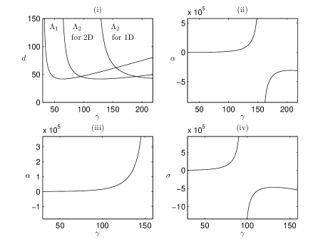
Figure 6. Gierer–Meinhardt equation with $a=\frac{1}{2}$, $b=1$. (i) Positive branches of $\Lambda_{1}$ and $\Lambda_{2}$ in one and two dimensions; (ii) Graph of $\alpha$ in the one-dimensional case; (iii) Graph of $\alpha$ in the two-dimensional case; (iv) Graph of $\sigma$ in the two-dimensional case.

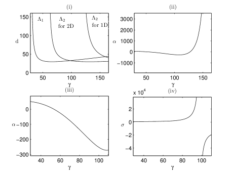
Figure 7. Gierer–Meinhardt equation with $a=\textstyle{\frac{1}{3}}$, $b=\textstyle{\frac{2}{3}}$. (i) Positive branches of $\Lambda_{1}$ and $\Lambda_{2}$ in one and two dimensions; (ii) Graph of $\alpha$ in the one-dimensional case; (iii) Graph of $\alpha$ in the two-dimensional case; (iv) Graph of $\sigma$ in the two-dimensional case.

7. Conclusions

In this paper we considered the evolution of an activator–inhibitor system consisting of two morphogens on a bounded domain subject to no-flux boundary conditions. Assuming that the system admits a uniform steady-state solution, which is stable in the absence of diffusion, we focused on solutions that bifurcate from this uniform steady-state solution. The bifurcation parameter $\lambda$ represented both $\gamma$, the ratio of the characteristic times for chemical reaction and diffusion, and $d$, the ratio of the diffusion coefficients of the two competing species (activator and inhibitor). We showed that, for such a system, there exists a critical curve $\Lambda_{1}$ in parameter space such that, as $\lambda$ crosses $\Lambda_{1}$, a bifurcation occurs (Lemma 3.1).

While a linear analysis around the uniform steady state suffices to obtain information about the formation of patterns, a nonlinear analysis is needed to gain insight into the long-time asymptotic behavior of the solutions after bifurcation. This issue is intimately connected with the long-term persistence of patterns.

In this paper we used the theory of attractor bifurcation, in combination with a center-manifold reduction, to analyze the long-time dynamics of bifurcated solutions. We considered two cases: diffusion on a (bounded) interval or a (non-square) rectangle, and diffusion on a square domain. In the former case, we showed that a bifurcation occurs as $\lambda$ crosses a critical curve $\Lambda_{1}$, and the bifurcation is a pitchfork bifurcation. Theorem 4.1 gives an explicit condition for the existence of an attractor. The attractor consists of exactly two steady-state points, each with its own basin of attraction. The two steady states correspond to patterns that differ only in phase; which of them is eventually realized depends on the initial conditions. Essentially the same conclusion holds in the case of diffusion on a rectangular (that is, non-square) domain; in particular, roll patterns emerge as a result of the bifurcation.

In the case of diffusion on a square domain, the dynamics are qualitatively different. Theorem 5.1 gives explicit conditions for the existence of an $S^{1}$-bifurcation. The bifurcated object consists of either an infinite number of steady states, or exactly eight regular steady-state points with heteroclinic orbits connecting them. Thus, two types of patterns may arise; for example, in the formation of animal coat patterns, we might expect stripe patterns or spot patterns.

Thus, in both the one- and two-dimensional case we have given a complete characterization of the bifurcated attractor and, therefore, of the long-time asymptotic dynamics of the bifurcated objects.

Appendix A Attractor Bifurcation and Reduction Methods

In this appendix, we summarize the attractor bifurcation theory of Ref. [11] and the reduction methods introduced in Ref. [12]. The functional framework is that of two Hilbert spaces, $H$ and $H_{1}$, where $H_{1}$ is dense in $H$ and the inclusion $H_{1}\hookrightarrow H$ is compact.

A.1. Attractor Bifurcation Theorem

Let $A:H_{1}\to H$ be a linear homeomorphism, and let $L_{\lambda}:H_{1}\to H$ be a compact perturbation of $A$ which depends continuously on a real parameter $\lambda$,

(A.1) $$L_{\lambda}=-A+B_{\lambda}.$$

The operator $L_{\lambda}$ is sectorial; it generates an analytic semigroup $S_{\lambda}(t)=\{e^{tL_{\lambda}}\}_{t\geq 0}$. Fractional powers $L_{\lambda}^{\alpha}$ are defined for all $\alpha\in[0,1]$; the domain of $L_{\lambda}^{\alpha}$ is $\mathrm{dom}(L_{\lambda}^{\alpha})=H_{\alpha}$, where $H_{0}=H$ and $H_{\alpha_{1}}\subset H_{\alpha_{2}}$ if $\alpha_{2}<\alpha_{1}$.

Let $G_{\lambda}:H_{\alpha}\to H$ be a nonlinear $C^{r}$-bounded map ($r\geq 1$) for some $\alpha\in[0,1)$, which depends continuously on $\lambda$ and satisfies the asymptotic estimate

(A.2) $$G_{\lambda}(w)=o(\|w\|_{H_{\alpha}}),$$

as $|w|\to 0$, uniformly in $\lambda$.

Let $w_{\lambda}(t;w_{0})\in H$ be a solution of the initial value problem

(A.3) $$\frac{dw}{dt}=L_{\lambda}w+G_{\lambda}(w),\;t>0;\quad w(0)=w_{0},$$

where $w_{0}\in H$ is given. In terms of $S_{\lambda}$, we have

(A.4) $$w_{\lambda}(t;w_{0})=S_{\lambda}(t)w_{0}+\int_{0}^{t}S_{\lambda}(t-s)G_{\lambda}(w_{\lambda}(s;w_{0}))ds,\quad t\geq 0.$$

Definition A.1.

(i)  A set $\Sigma\subset H$ is a (positive) invariant set of Eq. (A.3) if $S_{\lambda}(t)\Sigma=\Sigma$ for any $t\geq 0$. (ii)  An invariant set $\Sigma\subset H$ of Eq. (A.3) is an attractor if $\Sigma$ is compact and there exists a neighborhood $U\subset H$ of $\Sigma$ such that

$$\lim_{t\to\infty}\mathrm{dist}_{H}(w_{\lambda}(t;w_{0}),\Sigma)=0$$

for any $w_{0}\in U$. (iii)  The largest open set $U$ satisfying the above condition is the basin of attraction of $\Sigma$.

Definition A.2.

(i)  A solution $(w_{\lambda},\lambda)$ of Eq. (A.3) bifurcates from $(0,\lambda_{0})$ if there exists a sequence of invariant sets $\{\Omega_{n}\}$ of Eq. (A.3) with $0\notin\Omega_{n}$ such that

$$\lim_{n\to\infty}\max_{w\in\Omega_{n}}|w|=0,\quad\lim_{n\to\infty}\mathrm{dist}(\lambda_{n},\lambda_{0})=0.$$

(ii)  If the invariant sets $\Omega_{n}$ are attractors of Eq. (A.3), then the bifurcation is called an attractor bifurcation. (iii)  If the invariant sets $\Omega_{n}$ are attractors and are homotopy equivalent to an $m$-dimensional sphere $S^{m}$, then the bifurcation is called an $S^{m}$-attractor bifurcation.

The theory of Ref. [11] is developed under the conditions that (i) the spectrum of $A$ is discrete and consists of positive eigenvalues $\rho_{k}$ with corresponding eigenvectors $\varphi_{k}\in H_{1}$,

(A.5) $$A\varphi_{k}=\rho_{k}\varphi_{k},\quad k=1,2,\ldots,$$

where $0<\rho_{1}\leq\rho_{2}\leq\cdots\to\infty$; (ii) the vectors $\{\varphi_{k}\}_{k}$ form an orthogonal basis of $H$; and (iii) there exists a constant $\theta\in(0,1)$ such that $B_{\lambda}:H_{\theta}\to H$ is bounded uniformly in $\lambda$.

The eigenvalues of $L_{\lambda}$ are $\beta_{k}(\lambda)$, $k=1,2,\ldots$. The assumption is that there is a critical curve $\Lambda_{m}$ that separates the region $R_{m}$ where (the real parts of) the first $m$ eigenvalues are negative from the region $R_{m+1}$ where (the real parts of) the first $m$ eigenvalues are positive, and an exchange of stanility occurs if $\lambda=\lambda_{0}\in\Lambda_{m}$.

Theorem A.1 (Attractor Bifurcation Theorem [11]).

Let $\beta_{k}(\lambda)$, $k=1,2,\ldots\,$, be the eigenvalues of $L_{\lambda}$ (counting multiplicity). Suppose that, at some critical value $\lambda=\lambda_{0}$, the first $m$ eigenvalues $\beta_{1}(\lambda)$ through $\beta_{m}(\lambda)$ cross the imaginary axis into the right half of the complex plane, while the remaining eigenvalues, $\beta_{k}(\lambda)$ for $k=m+1,m+2,\ldots$, remain in the left half of the complex plane. Let $E_{1}$ be the eigenspace of $L_{\lambda}$ at $\lambda_{0}$,

$$E_{1}=\bigcup_{k=1}^{m}\left\{w\in H_{1}:(L_{\lambda_{0}}-\beta_{k}(\lambda_{0}))^{i}w=0,\,i=1,2,\ldots\right\},$$

and let $w=0$ be a locally asymptotically stable equilibrium point of Eq. (A.3) at $\lambda=\lambda_{0}$. Then

1. Eq. (A.3) bifurcates from $(w,\lambda)=(0,\lambda_{0})$ to an attractor $\mathcal{A}_{\lambda}$ as $\lambda$ transits from $R_{1}$ into $R_{2}$, $\dim\mathcal{A}_{\lambda}\in[m-1,m]$, and $\mathcal{A}_{\lambda}$ is connected if $m>1$;

2. $\mathcal{A}_{\lambda}$ is the limit of a sequence of nested $m$-dimensional annuli $M_{i}$ with $M_{i+1}\subset M_{i}$; in particular, if $\mathcal{A}_{\lambda}$ is a finite simplicial complex, then $\mathcal{A}_{\lambda}$ has the homotopy type of $S^{m-1}$;

3. For any $w_{\lambda}\in\mathcal{A}_{\lambda}$, $w_{\lambda}$ can be expressed as

   $$w_{\lambda}=W_{\lambda}+z_{\lambda},\quad W_{\lambda}\in E_{1},\quad z_{\lambda}=o(\|W_{\lambda}\|_{H});$$

4. There is an open set $U\subset H$ with $0\in U$ such that $\mathcal{A}_{\lambda}$ attracts $U\setminus\Gamma$, where $\Gamma$ is the stable manifold of $w=0$ with codimension $m$.

A.2. Reduction Method

A useful tool in the study of bifurcation problems is the reduction of the equation to its local center manifold. The idea is to project the equation to a finite-dimensional space after a change of basis; details can be found in [12].

Let $\lambda$ be close to a critical value $\lambda_{0}$. Suppose that the spaces $H$ and $H_{1}$ are decomposed,

(A.6) $$H=E_{1}\oplus E_{2},\quad H_{1}=\widetilde{E}_{1}\oplus\widetilde{E}_{2},$$

where $E_{1}$ and $E_{2}$ are invariant subspaces of $L_{\lambda}$, $E_{1}$ is finite dimensional, $\widetilde{E}_{1}=E_{1}$, and $\widetilde{E}_{2}$ is the closure of $E_{2}$ in $H$. The decomposition (A.6) reduces $L_{\lambda}$,

(A.7) $$L_{\lambda}=\mathcal{L}_{\lambda,1}\oplus\mathcal{L}_{\lambda,2},$$

where $\mathcal{L}_{\lambda,1}=L_{\lambda}|_{E_{1}}:E_{1}\to\widetilde{E}_{1}$ and $\mathcal{L}_{\lambda,2}=L_{\lambda}|_{E_{2}}:E_{2}\to\widetilde{E}_{2}$. If the decomposition is such that the real parts of the eigenvalues of $\mathcal{L}_{\lambda,1}$ are nonnegative at $\lambda=\lambda_{0}$, while those of $\mathcal{L}_{\lambda,1}$ are negative, then the solution $w_{\lambda}$ of Eq. (A.3) can be written as

(A.8) $$w=W+z,\quad W\in E_{1},\,z\in E_{2},$$

where $W$ and $z$ satisfy the system of equations

(A.9) $$\begin{split}\frac{dW}{dt}&=\mathcal{L}_{\lambda,1}W+\mathcal{G}_{\lambda,1}(W,z),\\ \frac{dz}{dt}&=\mathcal{L}_{\lambda,2}z+\mathcal{G}_{\lambda,2}(W,z),\end{split}$$

with $\mathcal{G}_{\lambda,i}=P_{i}G_{\lambda}$, $P_{i}:H\to\widetilde{E}_{i}$ being the canonical projection.

By the classical center-manifold theorem (see, for example, Refs. [7, 23]), there exist, for all $\lambda$ sufficiently close to $\lambda_{0}$, a neighborhood $U_{\lambda}\subset E_{1}$ of $W=0$ and a $C^{1}$ center-manifold function $\Phi^{\lambda}:U_{\lambda}\to E_{1}$, which depends continuously on $\lambda$, such that the dynamics of Eq. (A.3) are described completely by the dynamics of the finite-dimensional system

$$\frac{dW}{dt}=\mathcal{L}_{\lambda,1}W+\mathcal{G}_{\lambda,1}(W,\Phi^{\lambda}(W)),\quad W\in U_{\lambda}\subset E_{1}.$$

The following theorem gives an asymptotic approximation for $\Phi^{\lambda}$ as $\lambda\to\lambda_{0}$ or, alternatively, as $W\to 0$. The proof of the theorem is given in Ref. [12].

Theorem A.2.

Assume that $G_{\lambda}$, the nonlinear part of Eq. (A.3), is $C^{\infty}$, $G_{\lambda}(w)=\sum_{k=p}^{\infty}G_{\lambda,k}(w)$ for some $p\geq 2$, where $G_{\lambda,k}(w)=G_{\lambda,k}(w,\ldots,w)$, and $G_{\lambda,k}:H_{1}\times\ldots\times H_{1}\to H$ is a $k$-linear map. Then, under the conditions of Theorem A.1, the center-manifold function $\Phi^{\lambda}$ can be expressed as

$$\Phi^{\lambda}(W) =(-\mathcal{L}_{\lambda,2})^{-1}P_{2}G_{\lambda,p}(W)+O(|\Re\beta(\lambda)|\cdot||W||^{p})$$

$$\hskip 20.00003pt\mbox{}+o(||W||^{p}),\quad W\in E_{1},\;\lambda\to\lambda_{0},$$

where $\beta=(\beta_{1},\ldots\,,\beta_{m})$.

References

• [1] Benson, D. L., P. K. Maini, and J. A. Sherratt, Unravelling the Turing bifurcation using spatially varying diffusion coefficients, J. Math. Biol. 37, 381–417, 1998.
• [2] Bollerman, P., A. van Harten, and G. Schneider, On the Justification of the G-L Approximation in: Nonlinear Dynamics and Pattern Formation in the Natural Environment, A. Doelman and A. van Harten (eds.), Longman, 1995, pp. 20–36.
• [3] Cross, M. C. and P. C. Hohenberg Pattern formation outside of equilibrium Rev. Mod. Phys. 65, 851–1112, 1993.
• [4] Eckhaus, W. The Ginzburg–Landau manifold is an attractor J. Nonlinear Science 3, 329–348, 1993.
• [5] Gierer, A. and H. Meinhardt, A Theory of Biologocal Pattern Formation, Kybernetik 12, 30–39, 1972.
• [6] Haken, H. and H. Olbricht, Analytical Treatment of Pattern Formation in the Gierer–Meinhardt Model of Morphogenesis, J. Math. Biol. 6(4), 1978.
• [7] Henry, D., Geometric theory of semilinear parabolic equations, Lecture Notes in Mathematics, Vol. 840, Springer-Verlag, Berlin, 1981.
• [8] Hoyle, R. Pattern Formation, An Introduction to Methods, Cambridge University Press, 2006.
• [9] Iron, D., J. Wei, and M. Winter, Stability analysis of Turing patterns generated by the Schnakenberg model, J. Math. Biol. 49 (4), 358–390, 2004.
• [10] Koch, A.J. and H. Meinhardt, Biological Pattern Formation, Rev. Mod. Phys. 66, 1481–1508, 1994.
• [11] Ma, T. and S. Wang, Dynamic Bifurcation of Nonlinear Evolution Equations, Chin. Ann. Mathematics 26, 185–206, 2005.
• [12] Ma, T. and S. Wang, Bifurcation Theory and Applications, World Scientific, 2005.
• [13] Meinhardt, H., P. Prusinkiewicz, and D. R. Fowler, The Algorithmic Beauty of Sea Shells, Springer-Verlag, 2003.
• [14] Murray, J. D., Mathematical Biology II, third ed., Springer-Verlag, 2003.
• [15] Ni, Wei-Ming, Diffusion, cross-diffusion, and their spike-layer steady states, Notices Am. Math. Soc. 45, 9–18, 1998.
• [16] Ni, Wei-Ming, S. Kanako, and I. Takagi, The dynamics of a kinetic activator–inhibitor system, J. Diff. Eq. 229, 426–465, 2006.
• [17] Page, K. M., P. K. Maini, and N. A. M. Monk, Pattern formation in spatially heterogeneous Turing reaction–diffusion models, Physica D 181, 80–101, 2002.
• [18] Page, K. M., P. K. Maini, and N. A. M. Monk, Complex pattern formation in reaction–diffusion systems with spatially vaying diffusion coefficients, Physica D 202 95–115, 2005.
• [19] Schnakenberg, J., Simple Chemical Reaction Systems with Limit Cycle Behavior, J. Theor. Biol. 81, 389–400, 1979.
• [20] Schneider, G., Global existence via Ginzburg–Landau formalism and pseudo-orbits of G-L approximations, Comm. Math. Phys. 164, 157–179, 1994.
• [21] Schneider, G., Nonlinear diffusive stability of spatially-periodic solutions–abstract theorem and higher space dimensions, Tohoku Math. J. 8, 159–167, 1998.
• [22] Smoller, J., Shock Waves and Reaction–Diffusion Equations, second ed., Springer-Verlag, 1994.
• [23] Takagi, I., A priori estimates for stationary solutions of an activator–inhibitor model due to Gierer and Mainhardt, Tohoku Math. J. (2), 34(1), 113–132, 1982.
• [24] Turing, A., The Chemical Basis of Morphogenesis, Philos. Trans. Roy. Soc. London B 237, 37–52, 1952.
• [25] van Harten, A. On the validity of the Ginzburg–Landau equation J. Nonlinear Science 1, 397–422, 1991.
• [26] Wollkind, D. J., V. S. Manoranjan, and L. Zhang, Weakly Nonlinear Stability Analyses of Prototype Reaction–Diffusion Model Equations, SIAM Rev. 36, 176–214, 1994.
• [27] Zhu, M. and J.D. Murray, Parameter Domains for Generating Spatial Pattern, Int. J. Bifurcation and Chaos 5, 1503–1524, 1995.
Acknowledgments
The authors thank James Glazier (Indiana University), T. J. Kaper (Boston University) and A. Doelman (CWI, Amsterdam) for helpful discussions on the subject of pattern formation and for providing several of the references.
The work of H.G.K. was supported in part by the National Science Foundation under Award No. DMS-0549430-001 and by the U.S. Department of Energy under Contract No. DE-AC02-06CH11357. The work of S.W. and M.Y. was supported in part by the Office of Naval Research under contract N00014-05-1-0218 and by the National Science Foundation under contract DMS-0605067.
The submitted manuscript has been created in part by the UChicago Argonne, LLC, Operator of Argonne National Laboratory (”Argonne”) under Contract No. DE-AC02-06CH11357 with the U.S. Department of Energy. The U.S. Government retains for itself, and others acting on its behalf, a paid-up, nonexclusive, irrevocable worldwide license in said article to reproduce, prepare derivative works, distribute copies to the public, and perform publicly and display publicly, by or on behalf of the Government.