Signatures of fractal clustering of aerosols advected under gravity

Abstract

Aerosols under chaotic advection often approach a strange attractor. They move chaotically on this fractal set but, in the presence of gravity, they have a net vertical motion downwards. In practical situations, observational data may be available only at a given level, for example at the ground level. We uncover two fractal signatures of chaotic advection of aerosols under the action of gravity. Each one enables the computation of the fractal dimension $D_{0}$ of the strange attractor governing the advection dynamics from data obtained solely at a given level. We illustrate our theoretical findings with a numerical experiment and discuss their possible relevance to meteorology.

The transport of finite-size particles plays important role in several fields, from cloud physics malinowski to plankton dynamics plankt . The recent interest fsp_strange_attractors ; bec in this problem comes in part from the fact that the dynamics of these particles is dissipative due to the drag force. This makes dynamical systems tools and concepts, such as attractors and dimensions, applicable. In the presence of gravity, a net vertical motion occurs due to the density difference between fluid and particle. For heavy particles (aerosols), this leads to raindrop falling in the atmosphere prup and to the sedimentation of plankton plankt and marine snow marine_snow in the ocean.

In such situations, knowledge of the advection dynamics of the aerosols is of fundamental importance, whereas usually only data obtained at a given level (height) are available. This occurs often, for instance, in meteorology, in the case where the aerosols are raindrops. In fact, it is much easier to obtain direct measurements of the raindrops when they reach the ground level than before, i.e., when they are being advected in the air flow. The derivation of approaches to obtain information on the advection dynamics of aerosols solely from data observed at a given level is, therefore, an instrumental and relevant task. In particular, here we are interested in approaches to obtain the fractal dimension of the set where the aerosols cluster while they are advected.

We report the uncovering of two independent fractal signatures of chaotic advection under gravity. Both make the computation of the fractal dimension $D_{0}$ of the strange attractor in the $N$-dimensional configuration space possible without prior knowledge of the advection dynamics. First, we show that the time series of the instants of arrival of advected aerosols in a small detector placed at a given level has a fractal dimension which is equal to

$$d_{0}=1+D_{0}-N.$$ (1)

We assume that $D_{0}<N$, which implies that the attractor in the full $2N$-dimensional phase space is $D_{0}$-dimensional since a set of dimension $D_{0}$, when projected into a space of dimension $N$, typically remains $D_{0}$-dimensional if $D_{0}<N$ Falconer . Second, we show that the spatial distribution of the aerosols reaching a line at a given level contains discontinuities (jumps) at points that form a fractal set whose dimension is again equal to $d_{0}$ obs . We illustrate our findings with a numerical experiment.

The dimensionless form of the governing equation for the path ${\bf{r}}(t)$ of aerosols much denser than the fluid, subjected to Stokes drag and gravity, reads as maxey_riley :

$$\ddot{\bf r}=A\left({\bf u}-\dot{\bf r}-W{\bf n}\right),$$ (2)

where $\dot{\bf r}$ is the velocity of the aerosol, ${\bf u}={\bf u}({\bf r}(t),t)$ is the fluid velocity field evaluated at the position ${\bf r}(t)$ of the aerosol, and ${\bf n}$ is a unit vector pointing upwards in the vertical direction. Throughout this paper we consider the vertical direction along the axis $y$. The inertia parameter $A$ (larger values for smaller inertia) can be written in terms of the densities $\rho_{p}$ and $\rho_{f}$ of the aerosol and of the fluid, respectively, the radius $a$ of the aerosols, the fluid’s kinematic viscosity $\nu$, and the characteristic length $L$ and velocity $U$ of the flow. It is $A={R}/{St}$, where $R={\rho_{f}}/{\rho_{p}}\ll 1$ and $St=(2a^{2}U)/(9\nu L)$ is the Stokes’s number of the aerosol. As seen from (2), the gravitational parameter $W$ provides the dimensionless settling velocity in a medium at rest. The actual settling velocity is the result of two effects: the gravitational attraction (buoyancy) and an updraft, if present. We consider the settling velocity to be comparable with $U$, implying a $W$ of the order of unity.

For convenience, we treat the case where the fluid flow is two-dimensional, $N=2$. In this situation, the phase space of the advection dynamics of the aerosols is 4-dimensional, since the aerosols are not constrained to move with the same velocity as their corresponding fluid elements. For the sake of concreteness, let us consider the time-smoothened version of the alternating sinusoidal shear flow of Ref. pierrehumbert . In dimensionless form it is given as

$$\left\{\begin{array}[]{l}u_{x}({\bf r},t)=0.5\left(1+\tanh(\gamma\sin(2\pi t))\right)\sin(2\pi y),\\[8.5359pt] u_{y}({\bf r},t)=0.5(1-\tanh(\gamma\sin(2\pi t)))\sin(2\pi x).\end{array}\right.$$ (3)

This flow is defined on the unit square with periodic boundary conditions, and is periodic in time with a unit period. The vertical direction corresponds to the $y$-axis. Apart from the spatial (sinusoidal) factor, each velocity component consists of two plateaus in time with a rapid but smooth crossover if $\gamma=20/\pi$. This is a simple analytically given model which, nevertheless, possesses a paradigmatic property of both chaotic and turbulent flows Vil : the intense stretching of material elements.

Substituting Eq. (3) into Eq. (2) and fixing $R=10^{-3}$ and $W=0.8$, there are regions of the parameter $St$ for which the dynamics of the aerosols is ruled by a strange attractor. We note that the time-independence of the attractor’s dimension $D_{0}$, which will be essential in what follows, is valid for a broad class of randomly time-dependent flows as well (see conclusion). A bifurcation diagram and our analysis suggest the existence of strange attractors of dimension between 1 and 2 in an interval around $St=2\times 10^{-4}$ (apart, as usual, from some small periodic windows). Here we illustrate our general ideas by analyzing the strange attractor corresponding to $St=2\times 10^{-4}$, which is prototypical. Figure 1 shows four snapshots of the projection, $\Lambda$, of the strange attractor into the configuration space. Because of gravity, there is a net vertical motion of the fractal set of curves of $\Lambda$ downwards in Fig. 1. We compute the dimension of $\Lambda$ to be $D_{0}=1.79$.

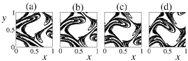
Figure 1: Snapshots, taken at (a) $t=0.65$, (b) $0.75$, (c) $0.85$ and (d) $0.95$, of the projection $\Lambda$ of the strange attractor into the configuration space.

Arrival times– The first fractal signature can be inferred from the following argument: Let us fix a point $P={\bf r}_{0}$ in the configuration space. Consider the product space of the configuration space and the time axis. In this space-time representation, the point $P$ corresponds to a $1$-dimensional straight line $({\bf r}_{0},t)$, $t\in\mathbb{R}$. The time coordinates of the set formed by the intersection of this line with the $(D_{0}+1)$-dimensional time-extension of $\Lambda$ correspond to the time instants of arrivals of aerosols at $P$. This intersection has a dimension Falconer given by $d_{0}=1+(D_{0}+1)-(N+1)$, since the time-extended configuration space is $(N+1)$-dimensional. Therefore, the time series of the instants of arrival of advected aerosols at the point $P$ has a fractal dimension $d_{0}$ given by (1).

For practical purposes, we substitute the point $P$ by a small codimension 1 object, placed horizontally, which is our detector. In the two-dimensional fluid flow that we analyze here, such object is a segment of length $\delta\ll L$. Seen at the scale of the detector, the dynamics of the advected aerosols under gravity roughly corresponds to a Cantor set of curves moving with some (both time and space dependent) horizontal velocity component $v_{h}$. The fractality of the time series of the instants of arrival of aerosols at the detector is measurable at scales $\tau>{\delta}/{v_{h}}$.

To validate numerically this fractal signature, we let $10^{6}$ aerosols, distributed on the attractor within the unit square at time zero, evolve until they reach the level $y=y_{0}=0$. Their instants of arrival as well as their $x$ coordinates are then recorded. We then choose a point $x_{0}$ and analyze the time series of instants of arrival at the segment $x\in(x_{0},x_{0}+\delta)$, $y=0$. The dimension $d_{ts}$ of this time series should, in face of our theoretical findings, be equal to $d_{0}=0.79$. We find excellent agreement with this value. For instance, taking $\delta=10^{-3}$, for $x_{0}=0.2$, $x_{0}=0.5$ and $x_{0}=0.8$, we find, respectively, $d_{ts}=0.80$, $d_{ts}=0.77$ and $d_{ts}=0.80$. The numbers of points in each of these choices of $x_{0}$ are, respectively, 185, 663 and 562. To calculate these dimensions, we have used the method described in grassberger_tel . This method is much more efficient than the usual box counting and is specially suited for computing the dimension of subsets of the real line. We explain it briefly here: Let us say that we want to measure the dimension $d$ of the set $M$. For each point $b_{i}\in M$, let $n_{i}(l)$ be the number of points in $M$ that lie within a distance $l$ of $b_{i}$. The following scaling can be shown to hold: $\langle 1/n(l)\rangle\sim{l^{-d}}$, where $d$ is the fractal dimension, and the bracket denotes a uniform averaging over all elements of the set. The dimensions for the different choices of $x_{0}$ were measured with $l\equiv\tau$ in the range $0.002<\tau<0.05$, equally spaced on the logarithmic scale.

Density jumps– The second fractal signature is associated with the spatial distribution $\mathbb{P}$ of the advected aerosols reaching a line $s$ at a certain level $y=y_{0}$ of the configuration space. Let ${\bf r}_{0}\in\mathbb{R}^{N-1}$ be the spatial coordinate of a point along a line $s$ at the $(N-1)$-dimensional plane $y=y_{0}$. We define $\mathbb{P}({\bf r}_{0})\mbox{d}{\bf r}$ as the probability that an aerosol reaches this plane in a $\mbox{d}{\bf r}$-neighborhood of the point ${\bf r}_{0}$ over a finite time interval $\Delta t$. $\mathbb{P}({\bf r}_{0})$ is proportional to the frequency of particles falling near ${\bf r}_{0}$, and can in principle be determined experimentally. The idea of the second signature is that the downward motion with local velocity ${\bf v}$ caused by gravity is equivalent to a projection of the whole fractal pattern shown in Figs. 1, 3(a), and 4 onto a horizontal line. As illustrated in Fig. 2, the direction of the projection is tangent to the distribution at a fractal set of points, which causes discontinuous jumps in the projected measure if $\Delta t$ is sufficiently large. This means that there is a fractal set of points where the density of detected particles has discontinuities. This is explained more rigorously in what follows, and we show that the fractal dimension of $\Lambda$ can be obtained from the dimension of the set of points where $\mathbb{P}$ changes discontinuously.

The attractor has an $SRB$-like measure srb , which is absolutely continuous (discontinuous) along the unstable (stable) foliation, and the distribution of points on $\Lambda$ inherits this property. The distribution $\mathbb{P}$ is proportional to the projected natural measure in the box of size $\mbox{d}{\bf r}$ around ${\bf r}_{0}$ on the level $y=y_{0}$ integrated over time. The measure is not continuous in the configuration space, but rather concentrated on the filaments of $\Lambda$. As a result, the distribution $\mathbb{P}$ can have a discontinuous jump where the local velocity ${\bf v}$ at a point of $\Lambda$ happens to be tangent to the corresponding filament. We call the points where this happens extremal points observation . In order to determine the dimension of such points, let us first consider a plane $(x,y)$ of the projected attractor (see Fig. 2). The extremal points of the main filaments can be joined by a smooth line $\xi$ (Fig. 2). The attractor’s dimension on this plane is $D_{0}+2-N$ (it is $D_{0}$ and $D_{0}-1$ for $N=2$ and $N=3$, respectively). Thus, the dimension of the extremal points on this plane is that of the intersection of a $1$ and a $D_{0}+2-N$-dimensional object, which is $1+(D_{0}+2-N)-2=D_{0}+1-N$. Next, observe that in the product space of the $x,y$ plane and the time axis this is a $D_{0}+2-N$-dimensional set. The points of line $s$ ($y=y_{0},z=$const) on which the distribution $\mathbb{P}$ is defined form a plane in this product space. Thus the set of points where the density jumps occur in the line $s$ at the fixed level $y=y_{0}$ has a dimension $2+(D_{0}+2-N)-3=D_{0}+1-N=d_{0}$.

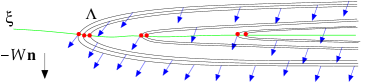
Figure 2: (color online) Illustration justifying the fractal signature on the density jumps. The black curves represent the slice $z=$const of $\Lambda$ at a certain time instant $t$. The vector field ${\bf v}$ defined on $\Lambda$ is represented by the blue arrows. Its tangencies with $\Lambda$ are the extremal points (red dots). The line $\xi$ (green) is a 1-dimensional line which joins all the extremal points of the $(x,y)$ plane.

The second fractal signature refers to a local property in the sense that it is related to discontinuities of a distribution. It is, therefore, intrinsically more difficult to detect in an experiment, due to the fluctuations induced by the finite number of observed aerosols. Such fluctuations tend to obscure the true discontinuities and lead to the consideration of points which do not correspond to true discontinuities. In principle, it can, however, be detected for a sufficiently large number of aerosols. To show this, consider the part of the attractor which is shown in black in Fig. 3(a). We let $1.7\times 10^{6}$ aerosols, forming that part of the attractor, evolve until they reach the line $y=y_{0}=0$. We measure the spatial distribution of the aerosols here using a sliding-window method, to be described now. We consider the segment $(0.88,0.98)\times 0$, which is divided into $10^{5}$ equal boxes $s_{i}$. We count the number $n_{i}$ of aerosols arriving in each $s_{i}$. We then define $r_{i}=\sum_{j=i}^{i+100}n_{j}$, $i=1,\cdots,10^{5}-100$, the total number of arrived aerosols in $100$ neighboring boxes. Next, consider $\Delta_{i}=r_{i+100}-r_{i}$, $i=1,\cdots,10^{5}-200$, the jumps between two adjacent intervals, each formed by $100$ boxes. Figure 3(b) shows $\Delta_{i}$ in the whole range. The local maxima are also indicated. We define a threshold $\alpha$ for these jumps and consider that the discontinuities in the spatial distribution occur at the points corresponding to the local maxima of $\Delta_{i}$ which exceed $\alpha$. The procedure is robust for $\alpha$ in a certain range that, at the same time, allows the detection of a reasonably large number of discontinuities and does not indicate false discontinuities (due to the fluctuations). In our numerical experiment, the minimum value of $\alpha$ for which no false discontinuity is detected is $204$. In this case, we find $51$ discontinuities. We compute the dimension $d_{sd}$ of this set of discontinuities. We obtain $d_{sd}=0.82$ over the range $0.0004<l<0.01$ in the interval $0.88<x<0.98$. The subset of $\Lambda$ reaching the line $y=0$ at the points where these discontinuities occur can be seen in Fig. 4. For $\alpha=218$, we find $47$ discontinuities, and the corresponding dimension is $d_{sd}=0.81$ over the same range. These dimensions are in very good agreement with the expected value $d_{0}=0.79$. For these computations, we use again the method of Ref. grassberger_tel .

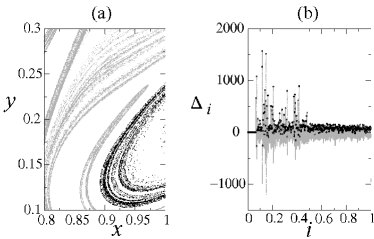
Figure 3: (a) Magnification of the snapshot $t=0.85$ of $\Lambda$ from Fig.1. Both the black and the gray points belong to $\Lambda$. The black points correspond to the part of the attractor which is used to illustrate the second fractal signature. (b) Density jumps $\Delta_{i}$ as a function of the box index $i$ (in units of $10^{5}$) (gray) along the line $s$ given by $y=y_{0}=0$. The local maxima are also shown (black dots).

Figure 4: Branch of $\Lambda$ at $t=0.85$ (gray and black points) from which the spatial distribution of aerosols is computed in the level $y=y_{0}=0$. The black subset reaches the level $y=0$ at the points where the density jumps ($\Delta_{i}>\alpha$) occur.

To summarize, we have shown that important information of the advection dynamics of aerosols in fractal sets can be obtained from data measured solely at a given level. We have uncovered two independent fractal signatures of chaotic advection under gravity. We have illustrated our fractal signatures using a flow model with periodic time-dependence, but our findings are far more general, since flows with random time-dependence (yet spatially smooth) also have the properties mentioned here. In particular, aerosols advected in such flows often approach a random attractor characterized by a well defined time-independent fractal dimension Rom ; SO ; bec . Note that the weight of the particles does not play a role in the argument. Therefore, the fractal signatures derived would also apply for the rising dynamics of finite-size particles lighter than the ambient fluid (bubbles). In fact, our fractal signatures are applicable to fractal chaotic attractors in general.

Our findings might be useful in meteorology, in the case where the aerosols are raindrops. Although our chaotic advection model neglects possibly important features of rain precipitation such as the spatial roughness of turbulent flows and the distribution of raindrop sizes, the fractal signature on the arrival times relies only on the time invariance of the dimension of the set where the aerosols accumulate. Therefore, if either the aforementioned mechanism based on the convergence of aerosols in random flows to strange attractors obs4 or any other mechanism leads to the accumulation of raindrops in fractal sets with a time-invariant dimension obs5 , then the signature on the arrival times may be used to characterize the fractal clustering of the raindrops. This signature could be measurable in precipitation data of rain, for instance, with the disdrometer which was used in the experiment reported in lavergnat . We note that a disdrometer was already used in Ref. zawadzki and even the correlation dimension ($D_{2}$) of a time series was measured and interpreted as a sign of irregular distribution of drops in space. Finally, we mention the experimental results of Ref. lavergnat showing a fractal dimension for the time series of arrival times of raindrops at a disdrometer (Fig. 9(a) of the cited reference). Both results lavergnat ; zawadzki are compatible with the accumulation of raindrops in fractal sets with a time-invariant dimension.

The authors thank I. Geresdi, I.J. Benczik, J. Davoudi, S.P. Malinowski, K. Gelfert, and an anonymous referee for useful discussions and suggestions. The support of FAPESP and CNPq (Brazil) and of the Hungarian Science Foundation (OTKA T047233, TS044839) are acknowledged. This work was partially done at Instituto de Física, Universidade de São Paulo, São Paulo, Brazil.

References

- (1) S.P. Malinowski et al., J. Atmos. Sci. 51, 397 (1994); P. Korczyk et al., Atmospheric Research 82, 173 (2006).
- (2) J. Ruiz et al., PNAS, 101, 17720 (2004).
- (3) L. Yu et al., Nonlinear Structure in Physical Systems, Eds. L. Lam and H.C. Morris (Springer-Verlag, New York, 1990), pp.223-231; P. Tanga and A. Provenzale, Physica (Amsterdam) 76D, 202 (1994); A. Babiano et al., Phys. Rev. Lett. 84, 5764 (2000); T. Nishikawa et al., Phys. Rev. Lett. 87, 038301 (2001); G. Falkovich et al., Nature 419, 151 (2002); I.J. Benczik et al., Phys. Rev. Lett. 89, 164501 (2002); C. Pasquero et al., Phys. Rev. Lett 91, 054502 (2003); K. Duncan et al., Phys. Rev. Lett 95, 240602 (2005).
- (4) J. Bec, Phys. Fluids 15, L81 (2003).
- (5) H.R. Pruppacher, Microphysics of Clouds and Precipitation (Kluwer Academic Publishers, Dordrecht, 1998).
- (6) T. Kiorboe and G.A. Jackson, Limnology and Oceanography, 46, 1309 (2001).
- (7) K. Falconer, Fractal Geometry (Wiley, Chichester, 1990); B.R. Hunt and V.Y. Kaloshin, Nonlinearity 10, 1031 (1997).
- (8) If the dimension of the strange attractor is smaller than , then Eq. (1) yields , implying that both the set of time instants of arrival of aerosols in a small detector and the set where discontinuities occur in the spatial distribution along a line at the fixed level are empty.
- (9) M.R. Maxey and J.J. Riley, Phys. Fluids 26, 883 (1983); T.R. Auton et al., J. Fluid. Mech. 197, 241 (1988); E.E. Michaelides, J. Fluids Eng. 119, 233 (1997).
- (10) R.T. Pierrehumbert, Chaos Solitons Fractals 4, 1091 (1994).
- (11) E. Villermaux et al., Mixing: Chaos and Turbulence, Eds. H. Chaté et al. (Kluwer Academic/Plenum publishers, New York, 1999), pp.1-8.
- (12) P. Grassberger, Chaos, Ed. A.V. Holden (Manchester Univ. Press, Manchester, U.K., 1986), pp. 291-311; T. Tél et al., Physica (Amsterdam) 159A, 155 (1989).
- (13) L.S. Young, J. Stat. Phys. 108, 733 (2002).
- (14) Whether an extremal point is actually associated with a density jump depends on whether it belongs or not to the line at the level .
- (15) F.J. Romeiras et al., Phys. Rev. A 41, 784 (1990).
- (16) J.C. Sommerer and E. Ott, Science 259, 335 (1993).
- (17) The parameters in our numerical experiment have been chosen to match raindrop data. For raindrops, typical numbers are and mm. Considering the advection of these drops by coherent structures of linear size m and typical velocity fluctuations m/s in atmospheric flows, we obtain and , since for air.
- (18) Fractal distribution of raindrops was investigated in S. Lovejoy et al., Phys. Rev. E 68, 025301(R) (2003) and M.L. Larsen et al., J. Atmos. Sci. 62, 4071 (2005).
- (19) J. Lavergnat and P. Gole, Journal of Applied Meteorology 37, 805 (1998).
- (20) I. Zawadzki, New Uncertainty Concepts in Hydrology and Hydrological Modeling, Ed. A.W. Kundzewicz (Cambridge U.P., Cambridge, 1995), pp. 104-108.