DFTT 4/07

Universal power law behaviors in genomic sequences and evolutionary models

Loredana Martignetti and Michele Caselle

Dipartimento di Fisica Teorica dell’Università di Torino and I.N.F.N.,

Via Pietro Giuria 1, I-10125 Torino, Italy

e–mail:          (caselle)(martigne)@to.infn.it

We study the length distribution of a particular class of DNA sequences known as 5’UTR exons. These exons belong to the messanger RNA of protein coding genes, but they are not coding (they are located upstream of the coding portion of the mRNA) and are thus less constrained from an evolutionary point of view. We show that both in mouse and in human these exons show a very clean power law decay in their length distribution and suggest a simple evolutionary model which may explain this finding. We conjecture that this power law behaviour could indeed be a general feature of higher eukaryotes.

1 Introduction

In these last years lot of efforts have been devoted in trying to find universal laws in nucleotide distributions in DNA sequences. A typical example was the identification more than ten years ago of long range correlations in the base composition of DNA (see for instance [1, 2] and references therein). With the availability of complete sequenced genomes, the correlation property of length sequences has been studied separately for coding and non coding segments of complete bacterial genomes, showing a rich variety of behaviour for different kinds of sequences [3, 4]. This line of research has been recently extended to the search of similar universal distribution for more complex features of eukaryotic DNA sequences like for instance 5’ untranslated regions (UTR) lengths [5], UTR introns [6] or strand asymmetries in nucleotide content [10, 7]. The main reason of interest for this type of analyses is the search of general rules behind the observed universal behaviours. The hope is to get in this way new insight in the evolutionary mechanisms shaping higher eukaryotes genomes and to understand functional role of the various portions of the genome. An intermediate important step of this process is the construction of simplified (and possibly exactly solvable) stochastic models to describe the observed behaviours. This is the case for instance of the model discussed in [8] for base pair correlations or the model proposed in [5] for the 5’UTR length. In this paper we describe a similar universal law for the exon length in the 5’UTR of the human and mouse genomes. Looking at the 5’UTR exons collected in the existing genome databases for the two organisms we shall first show that they follow with a high degree of confidence a power law distribution with a decay exponent of about $2.5$ and then suggest a simple solvable model to describe this behaviour.

We shall also compare the impressive stability of the power law decay of 5’UTR exons with the distributions in the case of the 3’UTR and coding exons which turn out to be completely different. This is most probably due to the different evolutionary pressures to which are subject the three types of sequences.

We think that the behaviour that we observed should indeed be a general feature of higher eukaryotes, however its identification requires a very careful annotation of 5’UTR regions which exist for the moment only for human and mouse (see tab. below).

This paper is organized as follows. After a short introduction to the biological aspects of the problem (sect. 2) we discuss the exon length distribution in sect.3 . Sect.4 is then devoted to the discussion of a simple stochastic model which gives as equilibrium distribution the observed power like behaviour. Details on the model are collected in the Appendix.

2 Biological background

In eukaryotic organisms, DNA information stored in genes is translated into proteins through a series of complex processes, carefully controlled at each step by specific regulatory mechanisms activated by the cell. In particular, two crucial events in this process are the production of an intermediate molecule, the messanger RNA (mRNA) transcript, and the translation of the mRNA into proteins. The cell provides fine regulatory systems to regulate the gene expression both at transcriptional and post-transcriptional level, using several cis–acting signals located in the DNA sequence. A common molecular basis for much of the control of gene expression (whether it occurs at the level of initiation of transcription, mRNA processing, translation or mRNA transport) is the binding of protein factors and specific RNA elements to regulatory nucleic acid sequences.

Once mRNA is transcribed, it usually contains not only the protein coding sequence, but also additional segments, which are transcribed but not translated, namely a flanking 5’ untranslated region (5’ UTR) and a final 3’ UTR . Nucleotide patterns or motifs located in 5’ UTRs and 3’ UTRs are known to play crucial roles in the post-transcriptional regulation. Most of the primary transcripts of euKaryotic genes also contain sequences (named “introns”) which are eliminated during a maturation process named “splicing”. The sequences which survive this splicing process are named ”exons” they are glued together by the splicing machinery and form the mature mRNA transcript. Both the UTRs and the coding portions of the mRNA are usually composed by the union of several exons. It is thus possible to classify the exons as coding, 3’UTR and 5’UTR depending on the portion of the mRNA to which they belong

A cell can splice the “primary transcript” in different ways and thereby make different polypeptide chains from the same gene (a process called alternative RNA splicing) and a substantial proportion of higher eukaryotic genes (at least a third of human genes, it is estimated) produce multiple proteins in this way (isoforms), thanks to special signals in primary mRNA transcripts.

Some hints about the 5’ and 3’ role in gene expression can be derived from a quantitative analysis of UTR length.

Recent large scale databases suggest that the mean 3’ UTR length in human transcript is nearly four times longer than the mean human 5’UTR length [9] and that the evolutionary expansion of 3’UTR in higher vertebrates, not observed in 5’ UTR, is associated to their peculiar regulatory role. Very recent works revealed the existence of an extremely important post-transcriptional regulatory mechanism, performed by an abundant class of small non coding RNA, known as microRNA (miRNA), that recognize and bind to multiple copies of partially complementary sites in 3’UTR of target transcripts, without involving 5’UTR [11, 12, 13].

Differently, 5’UTR sequences are expected to be constrained mainly by splicing process and translation efficiency. The exons in the 5’ UTR regions are usually termed “non coding exons”, since they are not included in the protein coding portion of the transcript. However, their characteristics, as their length, secondary structure and the presence of AUG triplets upstream of the true translation start in mRNA, known as upstream AUGs, have been shown to affect the efficiency of translation and to be preserved in the evolution of these sequences [14, 15, 5]. 5’UTR exons length can vary between few tens until hundreds of nucleotides, without typical length scale around favourite size, and the lower and upper bounds of this distribution is likely to be shaped by splicing and translation efficiency: exons that are too short (under 50 bp) leave no room for the spliceosomes (enzymes that perform the splicing) to operate [16], while exons that are too long can contain signals that affect translation efficiency. 5’UTR “non coding exons” are also free from selective pressure acting on coding exons, which strongly preserves the amminoacid information written in triplets of nucleotides in the protein coding exons.

For these reasons, in our analysis we decided to construct strictly disjoint subsets of exons, according to their position in the transcript (5’UTR exons, protein coding exons or 3’UTR exons). Moreover, we created a non redudant genome-wide datasets of exons, considering only one isoform for each gene, the most extended one.

Curated information about DNA sequences and annotation of eukaryotic organisms are provided by the Ensembl project, based on a software system which produces and maintains automatic annotation on selected eukaryotic genomes [17].

3 Analysis of exons distribution

We downloaded from the Ensembl database (release 40 [17]) all the available transcripts annotated as protein coding for different organisms, and we created a filtered dataset of non redundant exons, considering the most extended transcript for each gene. We eliminated all the exons with mixed annotations and grouped the remaining ones in three classes: 5’UTR, protein coding exons, and 3’UTR.

Plotting the length distribution of exons, separately for 5’UTR, coding exons and 3’UTR, we clearly observe different behaviours, which we think should reflect different evolutionary constrains acting on these classes of DNA sequences (Fig.1 a,b,c). In particular, the 5’ UTR exons size distribution shows a remarkably smooth power decay for large enough values of the exon length. To assess this point and to evaluate the threshold above which the power law behaviour starts, we fitted the observed distributions with a power law:

$$N(l)=l^{-\alpha}$$ (1)

where $N(l)$ is the number of exons of length $l$.

In order to evaluate the goodness of the fits that we performed, we divided the set of all exons into 18 equivalent bins and then assumed the variance of these bins as an indication of the statistical uncertainty of our estimates (results are independent from the binning choice). This allowed us to perform a meaningful $\chi^{2}$ test on the fits. This test is commonly used when an assumed distribution is evaluated against the observed data [18]. The quantity $\chi^{2}$ may be thought of as a measure of the discrepancy between the observed values and the respective expected values. It is convenient to compute the reduced chi square $\widetilde{\chi}^{2}$ (i.e. the ratio $\chi^{2}/(N_{p}-N_{f})$ where $N_{p}$ is the number of points included in the fit and $N_{f}$ the number of parameters of the fit). With this normalization one can immediately see if the fitting function correctly describes the data (which requires $\widetilde{\chi}^{2}\leq 1$). When instead $\widetilde{\chi}^{2}>1$ the absolute value of $\widetilde{\chi}^{2}$ gives a rough estimate of how inaccurate is the tested distribution to describe the data.

We fitted the data for the 5’UTR exons setting a minimum threshold on the exon length and then gradually increasing this threshold until a reduced $\widetilde{\chi}^{2}$ value smaller than one was obtained. The rationale behind this choice is that (as we shall see below) the power law decay is likely to be an asymptotic behaviour which is violated for short exon lengths. Starting from $l_{min}\sim 150$ both in human and in mouse good $\widetilde{\chi}^{2}$ values were obtained and we could estimate the critical index to be $\alpha\sim 2.5$. Detailed results of the fits are reported in Tab.1. The $\widetilde{\chi}^{2}$ values that we found support in a quantitative way the power law behaviour of the data, which was already evident looking at Fig.1a.

On the contrary, the coding exons and the 3’UTR exons length histograms display (on a ln-ln scale) non linear distributions with peaks of population around favourite sizes. In the range, where we are able to fit the power law decay of 5’UTR exons length, $\widetilde{\chi}^{2}$ values for linear fit in the other classes of exons are completely unacceptables (Tab. 2).

[] []

[]

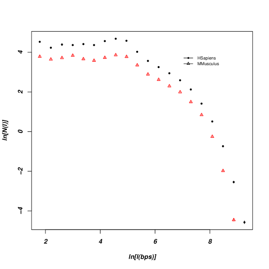
Figure 1: Exons length distribution in 5’UTR (a), protein coding exons (b) and 3’UTR (c) in human and mouse genome reported in ln-ln histograms (with bin size growing logaritmically). Plot errors are derived dividing the complete dataset in subsets of comparable dimension, avoiding biological biases, and averaging the length distribution of each subset.

Species	$\widetilde{\chi}^{2}$	$\alpha$ index	$lmin$ (bps)
H.Sapiens	0.52	2.56(2)	150
M.Musculus	0.74	2.61(2)	140

Table 1: Extimate of critical index $\alpha$ and length threshold $lmin$ for the power law distribution of 5’UTR exons in human and mouse

Species	protein coding exons	3’UTR exons	$lmin$ (bps)
H.Sapiens	84.37	13.46	150
M.Musculus	153.31	5.91	140

Table 2: $\widetilde{\chi}^{2}$ values for the linear fit of protein coding exons and 3’UTR exons length distribution, in the same range where we are able to fit the power law decay of 5’UTR exons length

The same plots for other organisms show exactly analogous trend, but they are affected by poor annotation of 5’ and 3’ UTR, which are very difficult to identify entirely (see Tab.3). In Tab. 3 we reported the total number of annotated protein coding genes, annotated 5’UTR and annotated 3’UTR for 4 different mammalian genomes, according to Ensemble database release 40. These data underline the current lack in the annotatation of 5’UTR and 3’UTR for other mammals, besides H. Sapiens and M. Musculus. For this reason, the same analysis performed for H. Sapiens and M. Musculus exon length distribution is prevented for other organisms.

Species	Annotated protein coding genes	Annotated 5’UTR	Annotated 3’UTR
H.Sapiens	23735	18333	18592
M.Musculus	24438	15945	16429
C.Familiaris	18214	5925	6298
G.Gallus	18632	7463	7670

Table 3: Annotated protein coding genes, 5’UTR and 3’UTR in Ensembl database release 40

In order to understand this peculiar behaviour of the 5’UTR exons we propose and discuss in the following section a simple model of exon evolution. Our goal is to understand if it is possible to associate the different behaviour that we observe to the greater freedom from selective pressure of the 5’UTR exons with respect to the coding and 3’UTR ones.

4 The model

Evolutionary models describe evolution of the DNA sequence as a series of stochastic mutations. There are three major classes of mutations: changes in the nucleotide type, insertions or deletions of one or more nucleotides. The various existing models differ with each other for the different assumptions they make on the parameter which control these changes (for a review see for instance [19, 20, 21]). From a biological point of view the two main assumptions of any evolutionary model are:

• evolution can be decribed as a Markov process, i.e. the modifications of a DNA sequence only depend on its current state and not on its previous history.

• evolution is “shaped” by functional constraints: DNA sequences with a negligible functional role evolve at a higher rate with respect of functionally important regions. This implies that regions with different functional roles must be described by different choices of the various mutational rates. The free evolution of sequences without functional constraints is usually called “neutral evolution”.

Let us see a few examples:

• protein coding exons are usually strongly constrained since the proteins they code have an important role in the life of the cell, however due to redundance of the genetic code, the third basis of each codon in the coding exons is free to mutate. On the contrary insertions and deletions are suppressed because they can dramatically affect the shape and function of the protein.

• Sequences devoted to transcriptional regulations (which very often lie outside exons) are usually so important for the life of the cell that they are kept almost unchanged over millions of years of evolution

• Regulatory sequences on the messanger RNA (mRNA) whose function often depends on the tridimensional shape of the RNA molecule and not on its exact sequence are in an intermediate situation between the above cases and the neutral evolution: they can tolerate mutations which do not modify their tridimensional shape (typically these are pairs of pointlike changes of bases and are usually called “compensatory mutations”). Most of the mRNA regulatory signals of this type are located in 3’UTR exons.

• 5’UTR regions contain sometimes regulatory sequences of the transcriptional type (which, as mentioned above, are stongly conserved under evolution) but their relative position seem not to have a crucial functional role. They can thus tolerate insertion and deletions as far as they do not affect the regulatory regions.

Since in our model we are only interested in the exon length distribution we may neglect the nucleotide changes and concentrate only on insertions and deletions. From this point of view, according to the above discussion both coding and 3’UTR should behave as highly constrained sequences while the 5’UTR ones should be more similar to the neutrally evolving ones. With this picture in mind we decided to model the neutral evolution of a DNA sequence under the effect of insertions and deletions only, to see which general behaviour one should expect for the length distribution and then compare it with the data discussed in the previous section.

To this end let us define $n_{j}$ as the number of 5’ UTR exons of length $j$ in the genome and let $N$ be the total number of such exons. Let $x_{j}\equiv n_{j}/N$ be the fraction of exons of length $j$.

If we assume that the exon length distribution evolves as a consequence of insertions and/or deletions of single nucleotides we find the following evolution equation for the $x_{j}(t)$ (where $t$ labels the time step of this process)

$$x_{j}(t+1)=x_{j}(t)+(j-1)\alpha x_{j-1}(t)-j\alpha x_{j}(t)+(j+1)\beta x_{j+1}(t)-j\beta x_{j}(t)$$ (2)

where $\alpha$ and $\beta$ denote the insertion and deletion probabilities respectively and we have kept into account the fact that for an exon of length $j$ there are exactly $j$ sites in which the new nucleotide can be inserted (i.e. that the insertion and deletion probabilities are linear functions of $j$, since the implied assumption is that all sites in our sequences are independent of one another).

At equilibrium the exon length distribution must satisfy the following equation (we omit the $t$ dependence which is now irrelevant)

$$(j-1)\alpha x_{j-1}-j\alpha x_{j}+(j+1)\beta x_{j+1}-j\beta x_{j}=0$$ (3)

It is easy to see that the only solution compatible with this equation is a power law of this type: $x_{j}=cj^{\eta}$ with $c$ a suitable normalization constant. Inserting this proposal in eq.(3) one immediatly finds $\eta=-1$.

This result is very robust, it does not depend on the values of $\alpha$ and $\beta$ and, what is more important, it holds also if instead of assuming the insertion (or deletion) of a single nucleotide, we assume the insertion or deletion of oligos (i.e. small sequences of nucleotides) of length $k$, with any choice of the probability distribution for the oligos length as fas as $k$ is much smaller than the typical exon length. Moreover one can also show that the power law decay still holds if we add to the process a fixed background probability of creation of new exons of random length as far as this probability is smaller than $x_{j_{max}}(\alpha-\beta)$ where $j_{max}$ is the largest exonic length for which the power law is still observed. This is rather important since it is known that retrotransposed repeats (in particular of the Alu family) may in some cases (with very low probability) become new active exons and represent one of the major sources of evolutionary changes in the transcriptome.

On the contrary this power law disappears if we assume that there is a finite probability that, as a consequence of the new insertion of deletion, the exon is eliminated. In this case the power law changes into a exponential distribution. This may explain why the power law decay is not observed in the coding and 3’UTR portion of the genes which are under a much stronger selective pressure (in the 3’UTR region are contained lot of post-trascriptional regulatory signals).

Since the critical index that we observe in the actual exon distribution in human and mouse is much larger than $1$ it is interesting to see which type of evolutionary mechanism could lead to a $\eta>1$ behaviour while keeping a power law decay. It is easy to see that this can be achieved assuming that the insertion (or deletion) probability is not linear with the length of the exon but behaves, say, as $p_{insertion}=\alpha j^{\lambda}$ with $\lambda>1$. Then, following the same derivation discussed above, we find at equilibrium an exon length distribution $x_{j}=cj^{-\lambda}$.

A possible explanation for such non-linear insertion rate comes from the observation that the transcribed portions of the genome (like the 5’ UTR exons in which we are interested), besides the normal mutation processes typical of the intergenic regions, are subject to specific mutation events due to the transcriptional machinery itself (see for instance [7]).

It is clear from the above discussion that in this case the critical index of the exon distribution, strictly speaking, is not any more an universal quantity, but depends on the particular biological process leading to the $p_{insertion}=\alpha j^{\lambda}$ probability discussed above. However it is conceivable that similar mechanisms should be at work in related species. This in our opinion explains why the critical indices associated to the mouse and human distributions are so similar and led us to conjecture that similar values should be found also in other mammalians as more and more 5’UTR sequences will be annotated.

Let us conclude by noticing that this whole derivation is based on the assumption that the system had reached its equilibrium distribution. This is by no means an obvious assumption and it is well possible that the fact that we observe a critical index larger than 1 simply denotes that the system is still slowly approaching the equilibrium distribution. There are three ways to address this issue. First one should extend the analysis to other organisms (however, as we discussed above, this will require a better annotation of the UTR regions in these organisms). Second one could reconstruct, by suitable aligning procedures, the UTR exons of the common ancestor between mouse and man and see if they also follow a power law distribution and, if this is the case, which is the critical index. Third one could simulate the model discussed above and look to the behaviour of the exon distribution as the equilibrium is approached. We plan to address these issue in a forthcoming publication.

Acknowledgements. This work was partially supported by FIRB grant RBNE03B8KK from the Italian Ministry for Education, University and Research.

The authors would like to thank D. Corà, E. Curiotto, F. DiCunto, I. Molineris, P. Provero, A. Re and G. Sales for useful discussions and suggestions.

Appendix A Derivation of the power law.

Inserting the distribution $x_{j}=cj^{\eta}$ in eq.(3) we find

$$\alpha(j-1)^{\eta+1}-\alpha(j)^{\eta+1}+\beta(j+1)^{\eta+1}-\beta(j)^{\eta+1}=0$$ (4)

which can be expanded in the large $j$ limit as

$$j^{\eta+1}\left[\alpha\left(1-\frac{\eta+1}{j}\right)-\alpha+\beta\left(1-\frac{\eta-1}{j}\right)-\beta\right]=0$$ (5)

which implies:

$$(\beta-\alpha)\frac{\eta+1}{j}=0$$ (6)

which (assuming $\beta\not=\alpha$) implies, as anticipated, $\eta=-1$.

A few observations are in order at this point:

a] It is clear from the derivation that the result is independent from the specific values of $\alpha$ and $\beta$ as far as they do not coincide. This independence from the details of the model holds also if we assume at each time step a finite, constant (i.e. not proportional to $j$) probability $\alpha^{\prime}~{}(\beta^{\prime})$ of random insertion (deletion) of a nucleotide. In this case the evolution equation becomes: equation becomes:

$$x_{j}(t+1)=x_{j}(t)+(j-1)\alpha x_{j-1}(t)-j\alpha x_{j}(t)+(j+1)\beta x_{j+1}(t)$$

$$-j\beta x_{j}(t)+\alpha^{\prime}(x_{j-1}(t)-x_{j}(t))+\beta^{\prime}(x_{j+1}(t)-x_{j}(t))$$ (7)

which still admits the same asymptotic distribution $x_{j}=cj^{-1}$

b] If we include a fixed exonization probability $p_{e}$ to create new exons from, say, duplicated or retrotransposed sequences the evolution equation changes trivially by simply adding such a constant contribution. The solution becomes in this case $x_{j}=cj^{-1}+d$ where the constant $d$ is related to $p_{e}$ as follows $d=p_{e}/(\alpha-\beta)$ and is negligible as far as it is smaller than $x_{j_{max}}$

c] Remarkably enough the above results are still valid even if the inserted (or deleted) sequence is composed by more than one nucleotide. Let us study as an example the situation in which we allow the insertion of oligos of length $k$ with $0<k<L$ and L smaller than the typical exon length. Let us assume for simplicity to neglect deletions and let us choose the same insertion probability $\alpha$ for all values of $k$. The evolution equation becomes:

$$x_{j}(t+1)=x_{j}(t)+\alpha\left[\sum_{k=1}^{L}x_{j-k}(t)(j-k)-Ljx_{j}(t)\right]$$ (8)

which implies

$$jx_{j}=\frac{1}{L}\sum_{k=1}^{L}(j-k)x_{j-k}$$ (9)

In the large $j$ limit this equation admits again a power law solution $x_{j}=cj^{\eta}$. Inserting this solution in eq.(8) we find

$$j^{\eta+1}\alpha\left[\frac{1}{L}\sum_{k=1}^{L}\left(1-\frac{k(\eta+1)}{j}\right)-1\right]=0$$ (10)

which is satisfied, as above, if we set $\eta=-1$.

d] On the contrary, if we assume a finite probability $(1-\gamma)$ of elimination of an exon as a consequnce of the insertion (or deletion) event (as one would expect if the sequence is under strong selective pressure) we find the following evolution equation:

$$x_{j}(t+1)=x_{j}(t)+[(j-1)\alpha x_{j-1}(t)\gamma-j\alpha x_{j}(t)]$$ (11)

where $\alpha$ is, as above, the insertion probability and we are assuming for simplicity single base insertions. This equation does not admit any more a power law solution at equilibrium but requires an exponential distribution: $x_{j}=e^{-\lambda j}j^{\eta}$ with $\eta=-1$ and $\lambda=ln(\gamma)$.

e] It is instructive to reobtain the result discussed in [a] above by looking at the equilibrium equation as a recursive equation in $j$:

$$x_{j+1}=\frac{j}{j+1}\left(1+\frac{\alpha}{\beta}\right)x_{j}-\frac{\alpha}{\beta}x_{j-1}~{}~{}~{}~{}(j>j_{min})$$ (12)

and

$$x_{j+1}=\frac{j}{j+1}(1+\frac{\alpha}{\beta})x_{j}~{}~{}~{}~{}(j=j_{min})$$ (13)

and construct recursively the solution for any $j$ starting from $x_{j_{min}}=c/j_{min}$. The recursion can be solved exactly and gives:

$$x_{j}=x_{j_{min}}\frac{j_{min}}{j}\frac{1-\left(\frac{\alpha}{\beta}\right)^{j-j_{min}+1}}{1-\frac{\alpha}{\beta}}$$ (14)

which (assuming $\alpha<\beta$)  leads asymptotically to the solution $x_{j}=c/j$ with $c=x_{j_{min}}\frac{j_{min}}{1-\alpha/\beta}$. This result allows to understand exactly the “finite size” corrections with respect to this asymptotic solution which turn out to be proportional to $\left(\frac{\alpha}{\beta}\right)^{j-j_{min}+1}$ and vanish if only deletions (i.e. $\alpha=0$) or only insertions (i.e. $\beta=0$) are present. In these cases the asymptotic solution is actually the exact equilibrium solution of the stochastic model.

References

- [1] W. Li, Comput Chem. 21, 257 (1997).
- [2] A. Arneodo, E. Bacry, P.V. Graves, J.F. Muzy, Phys Rev Lett. 74, 3293 (1995).
- [3] Zu-Guo Yu, V. V. Anh, and Bin Wang, Phys Rev E 63, 011903 (2000).
- [4] Zu-Guo Yu, V. V. Anh , Ka-Sing Lau, Physica A 301, 351 (2001).
- [5] M.L. Lynch, D.G. Scofield, X. Hong, Mol Bio Evo 22(4), 1137 (2005).
- [6] X. Hong, D.G. Scofield, M.L. Lynch, Mol Bio Evo 23(12), 2392 (2006).
- [7] M. Touchon, A. Arneodo, Y. d’Aubenton-Carafa, C. Thermes, Nucleic Acids Res. 32, 4969(2004).
- [8] P.W. Messer, P.F. Arndt, M. Lassig, Phys Rev Lett. 94(13), 138103 (2005).
- [9] G. Pesole, S. Liuni,G. Grillo, F. Licciulli,F. Mignone, C. Gissi, C. Saccone, Nucleic Acids Res. 30(1), 335 (2002).
- [10] M. Touchon,S. Nicolay,B. Audit,E.B. Brodie of Brodie,Y. d’Aubenton-Carafa, A. Arneodo, C. Thermes, Proc Natl Acad Sci U S A. 102(28), 9836 (2005).
- [11] D.P. Bartel, Cell 116(2), 281, (2004).
- [12] L. He,G.J. Hannon, Nat Rev Genet. 5(7), 522, (2004).
- [13] N. Rajewsky, Nat Genet. 38 Suppl:S8-13, (2006).
- [14] M. Iacono, F. Mignone, G. Pesole, Gene 349, 97 (2005).
- [15] A. Churbanov,I.B. Rogozin,V.N. Babenko,H. Ali,E.V. Koonin, Nucleic Acids Res. 33(17), 5512 (2005).
- [16] R. Sorek, R. Shamir, G. Ast, Trends Genet. 20(2), 68 (2004).
- [17] T. J. P. Hubbard & al., Nucleic Acids Res. Database issue (2007).
- [18] “Statistical methods in bioinformatics” W.J. Ewens, G.R. Grant Springer 2nd ed. (2005).
- [19] R. Durbin, S. Eddy, A. Krogh, G. Mitchison, “Biological Sequence Analysis: probabilistic models of DNA and protein sequences” Cambridge University Press (1998).
- [20] G. Mitchison, J. Mol. Evol. 49(1), 11 (1999).
- [21] C. Kosiol, L. Bofkin, S. Whelan, J. Biomed. Inform. 39(1) 51 (2006).