Some questions of Monte-Carlo modeling on nontrivial bundles

Abstract

In this work are considered some questions of Monte-Carlo modeling on nontrivial bundles. As a basic example is used problem of generation of straight lines in 3D space, related with modeling of interaction of a solid body with a flux of particles and with some other tasks. Space of lines used in given model is example of nontrivial fiber bundle, that is equivalent with tangent sheaf of a sphere.

1 Introduction

Monte-Carlo method, or method of statistical trials is a numerical method based on simulation by random variables and the construction of statistical estimators for the unknown quantities [1]. This method is used wider and wider due to permanent growth of capabilities and accessibility of computers and sometime is considered as a “brute force method” in comparison with more traditional analytical and numerical methods.

Such a critical view is not always justified and in the presented work is considered an example of practical task, when application of Monte-Carlo method is very naturally related with differential geometry and theory of fiber bundles.

One simplest application of Monte-Carlo method — is computation of multiple integrals. If it is required to estimate such an integral with respect to the Lebesgue measure in an $n$-dimensional Euclidean space, the generation of sequences of random points, distributed in such a space does not produce some specific problems.

As a basic example with a compact support may be considered the generation of uniformly distributed points in multidimensional rectangular area, represented as the direct product of $n$ intervals and containing given compact area. For generation of points with more general distribution laws may be used quite standard methods [2].

Such an approach does not produce especial difficulties, because a natural measure exists on Euclidean space and it specifies method of generation of uniformly distributed points, that may be used as a base for creation of more general distributions, produced via different transformations of the initial one.

It is more difficult to apply Monte-Carlo method to specific tasks, related with distributions of lines, planes, or other geometrical objects. A way to introduce a natural measure for such objects is not always obvious [3].

A classical example — is Bertrand paradox [3], associated with name of the French mathematician of XIX century (quite detailed discussion may be found also in [4, §19]). It is good illustration of considered class of problems.

The Bertrand problem is stated as finding probability for length of random chord in circle to be bigger than side of equilateral triangle, inscribed in given circle. It is called “paradox,” because alternative methods of solutions of given task produce different values for the probability. It is related with fact, that it is necessary first to define meaning of term “random” chord [3].

2 Straight lines in the space

The statement of the problem, illustrated in the example with Bertrand paradox, may be quite important for modeling of wide range of physical problems using Monte-Carlo method. Let us consider three-dimensional space ${\mathbb{R}}^{3}$ with a solid body and a distribution of random lines, corresponding to trajectories of particles, intersecting of given object.

It was already mentioned above, that it is necessary to describe precisely, which particular distribution of lines denoted as “random” and in presented work as basic example is considered isotropic uniform distribution of lines, defined by suggestion, that any points of space and any directions are equiprobable.

Despite of apparent simplicity of such definition, the example with Bertrand paradox shows necessity of accurate consideration. Say in Ref. [3] is suggested a general approach to description of geometric objects: first, to choose appropriate parametrization (co-ordinate system) for description of geometric object by unique way, and next, to define probability density function (measure) for given space of parameters.

As an example of given approach in Ref. [3] is considered description of a straight line in the space using equations:

$$\left\{\begin{array}[]{rclcl}x&=&a\,z&+&p\\ y&=&b\,z&+&q\end{array}\right..$$ (1)

Here $(a,b,p,q)$ — are four parameters describing the straight line in three-dimensional space $(x,y,z)$.

Invariant measure for considered parametrization $(a,b,p,q)$ Eq. (1) may be defined as [3, 5]:

$$(1+a^{2}+b^{2})^{-2}da\,db\,dp\,dq.$$ (2)

It should be mentioned, that parametrization Eq. (1) is not complete, because may not describe a set of lines those parallel to plane $z=0$.

For complete definition of manifold of straight lines in the space it may be used other method: to consider a plain $p$ containing origin of the co-ordinate system, point $q$ on the plane, and to draw straight line $l$ perpendicular to the plane through given point [5, 6] (see Fig. 1).

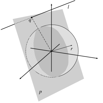
Figure 1: A line and a unit sphere of directions

This definition also specifies the space of lines as a four-dimensional manifold, because may be represented as a fiber bundle with two-dimensional base and two-dimensional fiber [6].

Really, any plane used in the definition may be presented by a straight line drawn through the origin of co-ordinate system and perpendicular to given plane. A space of such lines — is the projective space ${\mathbb{R}}P^{2}$, it is two-dimensional base of the fiber bundle. The two-dimensional fiber — is the plane itself.

Maybe more visual example is space of directed lines, corresponding to tangent sheaf of the sphere, where base is usual sphere and fibers — are tangent planes to the sphere [6].

3 Monte-Carlo method for space of lines

In applications with Monte-Carlo method, last definition produces following sequence of actions: to generate a unit vector (radius $\bm{r}$, Fig. 1); to draw the perpendicular plane $p$ through the origin of the coordinate system using the vector; to generate point $q$ on the plane; to draw (directed) line $l$ passing through given point and parallel to the vector.

Such a definition is convenient for modeling of isotropic uniform distribution of lines, because due to the symmetry reasons the both distribution of directions of the radii (points on sphere) and distribution of points on plane should be uniform.

This example displays specific properties, because tangent sheaf to the sphere (used for parametrization of space of straight lines), is not the trivial bundle. So generation of distributions using method described above may encounter some difficulties.

Really, straightforward approach could be described using procedure with two steps: to generate point uniformly distributed on unit sphere, to generate point uniformly distributed on plane (more exactly, on compact subset with size sufficient for modeling of particle flux for given volume).

Such a method meet a problem, because nontrivial bundle may not be presented as direct product of base on fiber and in general case probability distributions on fiber and base are not define distribution on total space.

The example with tangent bundle to the sphere is quite illustrative: a point on a tangent plane could be generated using two coordinates, if global fibration of tangent co-ordinate frames on sphere is given. But it is impossible to do it in some regular (continuous) way, because on the sphere may not exist a field of unit tangent vectors. It is so-called the hedgehog theorem [7, 8] (it is not possible to “comb” a hedgehog (ball), i.e., to arrange all spines smoothly).

In particular case of modeling of isotropic uniform distribution of lines using Monte-Carlo method there are few ways to avoid the problem. Say, it is possible to generate random tangent vector (or basis) for each plane. It is possible, because due to symmetry of the model, orientation of the basis does not matter. One method of construction of such random unit vector for arbitrary plane is: to generate random point in unit ball, to find projection on given plane and to normalize it on unit length.

From the one hand, this example shows specific advantages of Monte-Carlo method: it may be used even without proper parametrization of space of integration. For usual analytical methods it could appear necessity to use more difficult and indirect procedures, e.g., construction of atlas with few maps and transition functions for description of a fiber bundle [11] or deletion of part of space, similar with parametrization Eq. (1) above.

On the other hand, it would be convenient to have for arbitrary distribution on space of lines some general and regular procedure for Monte-Carlo method without suggestion about uniformity and isotropy of distribution of straight lines.

Let us consider fiber bundle used in given model with more details. It is convenient for simplicity again to use tangent sheaf of the sphere, corresponding to space of directed lines instead of initial fiber bundle over projective space.

It is known, that any fiber bundle may be defined as associated with some principal bundle [10], so it is convenient first to consider examples with principal bundles relevant to given problem.

By definition, the fiber of principal bundle — is Lie group, acting freely (without fixed points) on the space of the bundle. Two simple examples of principal bundles over the sphere [10] are frame bundle (it corresponds to a bundle of unit tangent vectors already mentioned before)

$${\mathbb{R}}P^{3}\cong SO(3)\stackrel{{\scriptstyle p}}{{\longrightarrow}}SO(3)/SO(2)\cong{\mathbb{S}}^{2}$$ (3)

with fiber is $SO(2)\cong{\mathbb{S}}^{1}$ and Hopf fibration [10, 12]

$${\mathbb{S}}^{3}\cong SU(2)\stackrel{{\scriptstyle p}}{{\longrightarrow}}SU(2)/U(1)\cong{\mathbb{S}}^{2}$$ (4)

with the same fiber $U(1)\cong{\mathbb{S}}^{1}$, represented as subgroup of diagonal matrixes in $SU(2)$ and base ${\mathbb{S}}^{2}$, but with different total space, (hyper)sphere ${\mathbb{S}}^{3}$.

The both cases are examples of principal bundles on homogeneous spaces, when space of bundle $G$ is Lie group, fiber $H$ is subgroup and base — is quotient space $M=G/H$. In such a case action of element of group $h\in H$ on space $G$ is expressed simply as right multiplication $G\ni g\mapsto gh$ [11].

One property of nontrivial principal bundles — is absence of continuous sections, i.e., maps from base to total space [11, 12]. Say, in the case with unit tangent vectors Eq. (3), such a map would produce tangent direction in any point of sphere and so the hedgehog theorem mentioned earlier is direct consequence of impossibility of such (continuous) section.

It is the demonstration of a principle, that some problems of Monte-Carlo modeling, discussed it presented work are really direct consequences of topological properties of fiber bundles.

Let us consider a problem of Monte-Carlo modeling of distribution of random tangent unit vectors on a sphere. For example, it is necessary to generate random direction and point on surface of ball with given probability distribution.

The fiber bundle is not trivial, and so for anisotropic distribution it is not simple not only resolve, but even state the problem, if to start from two independent distributions: points on sphere and points on circle (direction). It is an analogue of situation described above — it is not possible to build continuous global tangent coordinates on the sphere and so after generation of random point on a sphere and random direction (point on circle) it is not clear, how to “attach” given direction to given point on sphere (“Where is a North on the South Pole?”).

However, such a problem may be simple resolved, if to start with total space of the bundle. It is more correct way to state the tasks for Monte-Carlo method for such a cases. Say, for modeling of unit tangent vectors on a sphere, it is necessary to generate random element $A\in SO(3)$ (rotation).

Really, such an element has one-to-one correspondence with a frame $(\bm{x}^{\prime},\bm{y}^{\prime},\bm{z}^{\prime})$, produced via rotation $A$ from fixed standard co-ordinate frame $(\bm{x},\bm{y},\bm{z})$. Now, using the random (dashed) frame, it is possible to simply resolve given task: let $\bm{z}^{\prime}$ determines point on sphere, then $\bm{x}^{\prime}$ may be used as random direction from this point.

Though this method assumes possibility to specify distributions and generate random elements on the space ${\mathbb{R}}P^{3}\cong SO(3)$. For calculations and applications of Monte-Carlo method it is more convenient to start with space ${\mathbb{S}}^{3}\cong SU(2)$. The projective space ${\mathbb{R}}P^{3}$ may be produced from hypersphere ${\mathbb{S}}^{3}$ via identifying of all opposite points ${\mathbb{R}}P^{3}\cong{\mathbb{S}}^{3}/\{1,-1\}$ and, similarly, there is $2\to 1$ covering, homomorphism of groups, then the same rotation from group $SO(3)$ corresponds to two unitary $2\times 2$ matrixes: $a$ and $-a$ [13]

$$SO(3)\cong SU(2)/\{1,-1\}.$$ (5)

For treatment of the case with ${\mathbb{R}}P^{3}\cong SO(3)$ it is enough to consider distributions of random points on hypersphere ${\mathbb{S}}^{3}$ with densities satisfying property $\mu(\bm{r})=\mu(-\bm{r})$, where $\bm{r}$ is unit 4-vector, describing hypersphere in four-dimensional space.

Constructions are more difficult for associated bundles. Such a bundle is produced by following method [11]: if there is principal bundle $P$ with base $M$ and fiber (structure group) $G$, then for construction of associated bundle with the same base and fiber $F$ (with left action of $G$), the direct product $P\times F$ with action $(u,f)\mapsto(ug,g^{-1}f)$ is defined first, and it is considered quotient space with respect to such action $E=P\times_{G}F$. Now it is possible to represent $E$, as fiber space of bundle with base $M$ and fiber $F$ [10, 11].

An example of the associated bundle — is tangent sheaf to the sphere, used for description of space of (directed) lines. Formally, the construction described above may be used directly for description of arbitrary distributions on the tangent bundle of sphere.

Let us consider first the direct product $P\times F=SO(3)\times{\mathbb{R}}^{2}$. It is set of pairs $(g,r)$, $g\in SO(3)$, $r\in{\mathbb{R}}^{2}$. It is necessary now to introduce space $E$, i.e., quotient space on equivalence relation $(g,r)\sim(gh,h^{-1}r)$, there $h$ is element of group $SO(2)$, that is embedded in $SO(3)$ as subgroup of rotations around a fixed axis (say $\bm{z}$), on plane $SO(2)$ acts as rotations around origin.

The quotient space

$$E=SO(3)\times_{SO(2)}{\mathbb{R}}^{2}$$ (6)

has quite difficult structure and so for modeling of distributions on this space it is possible to use a method with invariant measure, already used earlier. Namely, any distribution on four-dimensional manifold $E$ may be identified with distribution on five-dimensional manifold $SO(3)\times{\mathbb{R}}^{2}$, with additional invariance property

$$\mu(g,r)\sim\mu(gh,h^{-1}r),\quad\forall\,h\in SO(2).$$ (7)

For applications to Monte-Carlo method such an algorithm may be described as follows: to generate random element of five-dimensional set $(A,r)\in SO(3)\times{\mathbb{R}}^{2}$ with distribution satisfying Eq. (7). The first element, $A\in SO(3)$, produces random frame $(\bm{x}^{\prime},\bm{y}^{\prime},\bm{z}^{\prime})$ and it was already discussed earlier in example with random tangent vector. The second element, $r\in{\mathbb{R}}^{2}$, describes point on plane. The first element also describes orientation of the plane via pair $(\bm{x}^{\prime},\bm{y}^{\prime})$, and it resolves the problem with lack of continuous tangent co-ordinate field on the sphere.

4 Conclusion

In this paper were considered some questions of Monte-Carlo modeling on nontrivial bundles. Though as the basic example was used distribution of straight lines in the space, it is possible to mention some general principles, which were used in presented work and may be applied in many other cases.

For consideration of nontrivial bundles it is useful to come from standard description, as projection from total space of bundle on a base [10], instead of less formal consideration of fiber bundle as some construction with base and fiber (aka “skew product”).

The definition of probability distribution on total space of the bundle always produces an adequate method of description, but separate constructions for distributions on base and fiber may be used either for trivial bundles (direct product of base and fiber), or for a case with invariance of distribution with respect to action of a structure group on the fiber, similarly with example of isotropic uniform distribution of lines.

Such a method is appropriate for spaces of bundles with simple geometrical structure, because it is necessary to have possibility of application of numerical methods for generation of distributions on these spaces. An example of such fiber bundles is the principal bundle on homogeneous spaces with not very complicated Lie groups, e.g., Hopf fibration discussed above Eq. (4).

Yet another method used in present work for description of associated bundles — is consideration of invariant densities Eq. (7). This method also may be used in many other cases, because in definition of associated bundles is used quotient space $E=P\times_{G}F$.

Notes: The presentation of the problem here should not be considered as multifold. On the one hand, often may be used simplified approach with modeling of isotropic uniform distribution of lines inside of a sphere via surface source on the sphere with cosine angular distribution [14]. It is yet another example of incomplete parametrization of space of lines. On the other hand, instead of using associate bundle Eq. (6) space of lines may be presented directly as quotient space of group $ISO(3)$ of all isometries of ${\mathbb{R}}^{3}$ [15] or described using theory of complex surfaces and twistors [16].

References

- [1] G. A. Mikhailov, Monte-Carlo method in M. Hazewinkel (ed), Encyclopaedia of mathematics, (Springer–Verlag, Berlin, 2002).
- [2] M. Abramowitz and I. A. Stegun (ed.), Handbook of mathematical functions (U.S. National Bureau of Standards, Washington, 1964).
- [3] M. G. Kendall and P. A. P. Morran, Geometrical probability, (Griffin, London, 1963).
- [4] M. Gardner, “Probability and ambiguity,” in The second Scientific American book of mathematical puzzles and diversions, (Simon & Schuster, New York, 1961; University of Chicago Press, Chicago, 1987).
- [5] L. A. Santaló, Integral geometry and geometric probability, (Addison–Wesley, Reading, 1976).
- [6] R. V. Ambartsumyan, et. al. Introduction to stochastic geometry, (Moscow, Nauka, 1989) [Rus.].
- [7] M. M. Postnikov, Lectures on algebraic topology. Homotopy theory of cell complexes, (Nauka, Moscow, 1988) [Rus.].
- [8] L. E. J. Brouwer, “Üeber Abbildungen von Mannigfaltigkeiten,” Math. Ann., 71, 97–115 (1912) [Deu.].
- [9] M. M. Postnikov, Lectures on geometry. Semester IV. Differential geometry, (Nauka, Moscow, 1988) [Rus.]; (Mir, Moscow, 1994) [Fr.].
- [10] B. A. Dubrovin, A. T. Fomenko, and S. P. Novikov, Modern geometry — Methods and applications, (Nauka, Moscow, 1986) [Rus.]; (Springer–Verlag, Berlin, 1984) [Eng.]
- [11] S. Kobayashi and K. Nomizu, Foundations of differential geometry, v. I, (Interscience Publ., New York, 1963).
- [12] N. Steenrod, The topology of fiber bundles, (Princeton University Press, Princeton, 1951).
- [13] M. M Postnikov, Lectures on geometry. Semester V. Lie groups and Lie algebras, (Nauka, Moscow, 1982) [Rus.]; (Mir, Moscow, 1986) [Eng.].
- [14] A. M. Kellerer, “Consideration on the random traversal of convex bodies and solutions for general cylinders,” Radiat. Res., 47, 359–376 (1971).
- [15] S. Helgason, Groups and geometric analysis, (Academic Press, New York, 1984).
- [16] N. J. Hitchin, “Monopoles and geodesics,” Comm. Math. Phys., 83, 579–602 (1982).