The role of the slope of ‘realistic’ potential barriers
in preventing relativistic tunnelling in the Klein zone

Abstract

The transmission of fermions of mass $m$ and energy $E$ through an electrostatic potential barrier of rectangular shape (i.e. supporting an infinite electric field), of height $U>E+m\,c^{2}$ - due to the many-body nature of the Dirac equation evidentiated by the Klein paradox - has been widely studied. We exploit here the analytical solution, given by Sauter for the linearly rising potential step, to show that the tunnelling rate through a more realistic trapezoidal barrier is exponentially depressed, as soon as the length of the regions supporting a finite electric field exceeds the Compton wavelenght of the particle - the latter circumstance being hardly escapable in most realistic cases.

PACS numbers 03.65.Pm, 03.65.Xp

I Introduction and main result

We will consider a one-dimensional flux of free monoenergetic electrons of energy $E$ and momentum

$$p=\sqrt{E^{2}-m^{2}}$$ (1)

(throughout the paper natural units $\hbar=c=1$ will be used) hitting a repulsive rectangular potential step of height $U$ greater than their kinetic energy $E-m$ (Fig. 1) - to which they are minimally coupled. In this case total reflection is unavoidable: in the region $x>0$ there is indeed just one bounded solution of the Schrödinger equation and the flux is therefore zero. As a consequence, in the region $x<0$ the reflected flux must equal the incident one.

Figure 1: Klein step

The use of the Schrödinger equation is legitimate as long as both $U,\,E-m\ll m$ and, in principle, the result must not necessarily hold for higher values of $U$. Indeed for

$$U-m>E>m\qquad{\rm(Klein\ zone)}$$ (2)

(the only zone we will be interested in throught the paper) a relativistic equation is more suited for the description of the situation and, for both the Klein-Gordon and the Dirac equation (to which our discussion will be limited), it happens that in the region $x>0$ the plane-wave (free propagation) solutions with opposite momenta $\pm q$,

$$q=\sqrt{(U-E)^{2}-m^{2}}$$ (3)

are two. Therefore the possibility of a non trivial transmitted flux of the same order of magnitude as the incident one is re-opened. The first to point out such a seemingly paradoxical result was Klein KL in the case of the then recently proposed Dirac equation.

Figure 2: Sauter step

The result has been commented upon and used by several authors over the years: see e.g. ref. CalDom for a historical review and some references. For us it is important to mention that Klein’s result was questioned by Sauter SA who, following a suggestion by Bohr, showed - at least for the Dirac equation - that, when the sharp edge of the step is substituted by a more realistic one of width $\ell$ (FIG. 2), the transmission coefficient turns out to be

$$T^{\rm Sauter\ step}_{\rm D}\simeq e^{-\pi\,m^{2}\,\ell/U}\ .$$ (4)

The asymptotic form exhibited in (4) holds when both the particles are fast $E-m\simeq m$ and the slope of the step, i.e. the electric field, satisfies

$$e\,{\cal E}=U/\ell\ll 2m/\lambda_{\rm Compton}=2m^{2}\,.$$ (5)

A discussion, in the above framework, of whether the Klein paradox is a ‘real’ one and - at least for the Dirac equation - Sauter’s is the right way out, cannot help spelling out what particles do the asymptotic states describe. Indeed, while in the region $x<0$ the dispersion relation $E=+\sqrt{p^{2}+m^{2}}$ is unambiguous, in the region $x>\ell$, owing to (2) and (3), either

$$E=U-\sqrt{q^{2}+m^{2}}$$ (6)

or

$$-E=-U+\sqrt{q^{2}+m^{2}}\ .$$ (7)

Namely either particles have negative kinetic energies, or antiparticles (propagating backward in time) have to come into play: the first choice being untenable, the many-body nature of both relativistic equations can no longer be ignored.

Postponing the discussion of this point until Section II, we prefer instead to examine the Klein paradox in the context of a different ‘Gedanken’ experiment where it is possible, for a while, to “sweep the dust under the rug”: can an appreciable fraction of monoenergetic electrons pass through a potential barrier of height $U\gtrsim 2m\,$?

Figure 3: Klein barrier

The situation is summarized in FIG.s 3 and 4. The former is the well studied rectangular barrier of width $2L$ whose transmission coefficient is known both in the Klein-Gordon and Dirac case:

$$T_{\pm}^{\rm rect\ bar}=\frac{1}{1+f_{\pm}(E,U)\,\sin^{2}(2q\,L)}$$ (8)

$$f_{\pm}(E,U)=\begin{cases}\displaystyle{\frac{U^{2}(U/2-E)^{2}}{p^{2}\,q^{2}}}&\qquad+=\text{KG}\\ \\ \displaystyle{\frac{m^{2}\,U^{2}}{p^{2}\,q^{2}}}&\qquad-=\text{D}\end{cases}$$ (9)

$p,\ q$ being given by (1), (3) respectively. This is the schematization of ‘infinite electric field’: the width of the edges of the barrier is neglected with an ensuing electric field much higher then its relevant scale $2m^{2}/e$ given in (5). This limitation is instead removed in the case of the trapezium shaped potential of Fig. 4, the extension of Sauter’s cure to the barrier. It is our choice to preserve space inversion as a symmetry (it will be evident that our conclusion does not critically depend on this assumption) and we will nickname this potential as Sauter barrier.

Figure 4: Sauter barrier

The advantage of barriers with respect to steps is that in both the regions where $U=0$, one may choose asymptotic states describing particles and ignore ‘what is going on under the barrier’ (we mean $-L<x<L$), i.e. whether either particles or antiparticles and/or couples are freely propagating.

This aspect has been examined in KSG for the step, in dLR for the barrier, by adopting a space-time description of the scattering process instead of the stationary state picture we are sticking to here.

Also the authors of dLR claim a ‘barrier paradox’. How does the paradox show up in the case of the rectangular barrier? Firstly it will be noted in (8) that for the values of $E$ such that $2q\,L=n\,\pi$, $n$ integer, there is total transmission (the so-called transmission resonances), both in the Klein-Gordon and the Dirac case, no matter how high the values of $U$ and $L$ may be. This is in blatant contrast with the Schrödinger case mentioned in the beginning. A second crucial difference is in the role played by the barrier width parameter $L$. While its increase induces the well known exponential decrease of $T^{\rm rect\ bar}_{\rm Schroedinger}$, in both the relativistic cases - for fixed $U$ - the higher the value of $L$, the faster the oscillations of $T_{\pm}^{\rm rect\ bar}$ as a function of $E$. Fig.s 5 and 6 illustrate this statement.

To make our point we have now to take into account how a ‘realistic’ experiment would be carried out and to give the numerical values of the scales involved.

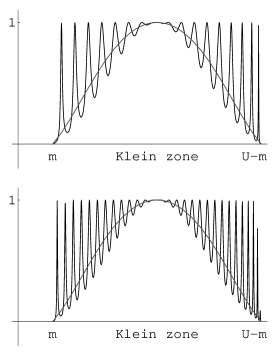
Figure 5: $T^{\rm rect\ barr}_{\rm KG}$ as a function of $E$ in the Klein zone: $U=8m$, $L=4/m$ (up) and $L=6.5/m$ (down)

Figure 6: $T^{\rm rect\,barr}_{\rm D}$ as a function of $E$ in the Klein zone: $U=8m$, $L=4/m$ (up) and $L=6.5/m$ (down)

Taking $L\gg 1/m=\lambda_{\rm Compton}=0.024$ Å for electrons (and smaller for more massive bosons) is simply mandatory. In addition, in a ‘real experiment’, where almost monoenergetic particles - with average energy $\overline{E}$ and an energy uncertainty $\Delta E\ll\overline{E}$ - are gunned against the barrier, the in-state is obtained as some superposition of stationary states with $\overline{E}-\frac{1}{2}\Delta E\lesssim E\lesssim\overline{E}+\frac{1}{2}\Delta E$. Thus, even for reasonably monoenergetic electrons, a huge number of transmission resonances is involved in the diffusion process. As an example, for $m=0.51$ MeV, $U\geq 1.2$ MeV, $L\geq 10$ Å and $\overline{E}\simeq m+\frac{1}{2}\Delta E=0.520$ MeV (i.e. at the very beginning of the Klein zone with a relative monoenergeticity $\Delta E/\overline{E}\leq 4\%$) no less than 1450 spikes in the analogues of Fig.s 5 and 6 are involved.

Such fast oscillations have to be taken into account CalDom . This is done by replacing the $\sin^{2}(\dots)$ with $\frac{1}{2}$ in (8) and this, in turn, leads to an energy-averaged transmission coefficient

$$\overline{T}_{\pm}^{\,{\rm rect\ bar}}\equiv\frac{1}{1+\frac{1}{2}\,f_{\pm}(\overline{E},U)}\cdot$$ (10)

(the non-oscillating curve in Fig. 5 and 6). As long as $\overline{T}_{\pm}^{\rm rect\ bar}$ is taken as an indicative prediction of the theory, the seeming paradox shows up in the following way:

$$\overline{T}_{\pm}^{\,{\rm rect\ bar}}\quad\stackrel{{\scriptstyle U\gg\overline{E}}}{{\longrightarrow}}\quad\begin{cases}0\\ \displaystyle{\frac{\overline{E}^{\,2}-m^{2}}{\overline{E}^{\,2}-m^{2}/2}}\ \stackrel{{\scriptstyle\overline{p}^{\,2}\ll m^{2}}}{{\longrightarrow}}\ 2\,\frac{\overline{p}^{\,2}}{m^{2}}\end{cases}$$ (11)

indicating an ‘unnaturally’ high transmittivity of Dirac particles in presence of a high step. The ‘unnatural’ is referred to the comparison with the exponentially small Schrödinger prediction. Even without going to the first limit taken in (11), for example, for $U=2.5$ MeV and average kinetic energy $\overline{E}-m=0.1$ MeV, the 31.3% of the incident flux would be transmitted, the fraction going up to 64.7% for $\overline{E}-m=0.5$ MeV.

The present paper addresses the question of whether Sauter’s cure for the barrier is as good as it is for the step. In addition to giving the analytical result for $T^{\rm Sauter\ barr}_{\rm D}$, our main result consists in showing that, for the Sauter barrier, in the part of the Klein zone where $E-m\simeq m$,

$$\overline{T}^{\,\rm Sauter\ barr}_{\rm D}\propto\,(T^{\rm Sauter\ step}_{\rm D})^{2}\propto e^{-2\pi\,m^{2}\,\ell/U}$$ (12)

provided the slope $\ell$ is large enough so as to satisfy (5).

As a matter of fact, for devices involving either macro or mesoscopic dimensions, the result (12) is a doom: for practical purposes transmittivity is zero, in accordance with the naive expectation. Should one ever be able to set up a nanostructure with $\ell$ as small as $10^{\,2\div 3}\lambda_{\rm Compton}$ and $U$ not much higher than the threshold $2m$, it is seen that the constraint (5) would be - even in this case - largely satisfied. Cases that could possibly be left uncovered by the present discussion are those of solid state physics where the ‘effective mass’ of the electron is smaller than the in-vacuum-value adopted here. In particular the case of graphene, where a vanishing effective mass is advocated by the authors of Ref. graphene , looks to date as the most promising ground where to observe the Klein paradox at work and, in the most optimistic case, to set up a “graphene device electronics” grapheneBis .

The paper is organised as follows.

In Section II the transfer matrix $M^{\rm step}$ for a generic potential step is defined and the corresponding transmission coefficient discussed. In Section III the tranfer matrix and transmission coefficient for the corresponding space-inversion invariant barrier are expressed in terms of the matrix elements of $M^{\rm step}$. Section IV (relying on the analytical results extracted from Sauter’s original paper and collected in the Appendix) illustrates the case of Sauter’s trapezoidal barrier and justifies why the averanging procedure described for (10) applies and how is it that (12) finally comes about.

II Steps

The present section contains material that is well known: as it mainly serves to introduce our notation, some of the statements to be found below will be made without proof. For the sake of conciseness we give a unified treatment of the Klein-Gordon equation in the first-order formalism and of the Dirac equation, in one space dimension. In the latter case we make use of two-component spinors since the spin - conserved by minimal coupling - is irrelevant. We will make use of the Pauli matrices:

$$\sigma_{1}=\begin{pmatrix}0&1\\ 1&0\end{pmatrix},\,\sigma_{2}=\begin{pmatrix}0&-i\\ i&0\end{pmatrix},\,\sigma_{3}=\begin{pmatrix}1&0\\ 0&-1\end{pmatrix}$$

as well as of the $2\times 2$ identity matrix $I$.

We are interested in the stationary states

$$\Psi_{E}(x,t)=e^{-i\,E\,t}\,\Psi_{E}(x)\,,\quad\Psi_{E}(x)=\begin{pmatrix}\psi_{E}(x)\\ \chi_{E}(x)\end{pmatrix}$$ (13)

of the Klein-Gordon one-dimensional wave equation

$$\begin{cases}\psi_{E}^{\prime}=\chi_{E}\\ \chi_{E}^{\prime}=-\Big{(}\!\big{(}E-U(x)\big{)}^{2}-m^{2}\Big{)}\,\psi_{E}(x)\end{cases}$$ (14)

as well as of the Dirac equation. In the Pauli representation the one-dimensional Dirac Hamiltonian is

$$H_{\rm D}^{\rm Pauli}=-i\,\sigma_{1}\,\frac{d}{dx}+\sigma_{3}\,m+U(x)$$ (15)

i.e., spelling out the components,

$$\begin{cases}\psi_{E}^{\prime}=i\,\big{(}E+m-U(x)\big{)}\,\chi_{E}\\ \chi_{E}^{\prime}=i\,\big{(}E-m-U(x)\big{)}\,\psi_{E}\ .\end{cases}$$ (16)

In both (14) and (16) the energy $E$ is understood to be in the Klein zone (2) and the step potential $U(x)$ is given by

$$U(x)=\begin{cases}0&x<0\\ {\cal U}(x)&0<x<\ell\\ U&x>\ell\ .\end{cases}$$ (17)

The solutions of the above equations may all be expressed in the form

$$\Psi_{E}=\begin{cases}\alpha\,u(p)\,e^{i\,p\,x}+\beta\,u(-p)\,e^{-i\,p\,x}&x<0\\ \Xi(x)&0<x<\ell\\ \gamma\,u(q)\,e^{i\,q\,x}+\delta\,u(-q)\,e^{-i\,q\,x}x>\ell\end{cases}$$ (18)

where $\Xi(x)$, representing the solution in the intermediate region, evidently depends on the explicit form of ${\cal U}(x)$. The momenta $p$, $q$ are given by (1), (3), and the two component wave functions are respectively

$$u_{\rm KG}(\pm p)=\begin{pmatrix}1\\ \\ \pm i\,p\end{pmatrix} \,,\quad u_{\rm D}(\pm p)=\begin{pmatrix}1\\ \\ \displaystyle\frac{\pm p}{E+m}\end{pmatrix}$$ (19)

$$u_{\rm KG}(\pm q)=\begin{pmatrix}1\\ \\ \pm i\,q\end{pmatrix} \,,\quad u_{\rm D}(\pm q)=\begin{pmatrix}1\\ \\ \displaystyle{\frac{\pm q}{E-U+m}}\end{pmatrix}\!\cdot$$ (20)

Imposing the continuity of $\Psi_{E}$ at the points $x=0,\,x=\ell$ entails two relations of linear dependence among the four constants $\alpha,\,\beta,\,\gamma,\,\delta$. The transfer matrix $M^{\rm step}$, expressing such a dependence, is defined by

$$\begin{pmatrix}\gamma\\ \delta\end{pmatrix}=M^{\rm step}\,\begin{pmatrix}\alpha\\ \beta\end{pmatrix}=\begin{pmatrix}a&b\\ c&d\end{pmatrix}\begin{pmatrix}\alpha\\ \beta\end{pmatrix}\cdot$$ (21)

Use of the invariance of (14) and (16) under charge conjugations

$${\cal C}:\quad\Psi(x)\to C\,\Psi^{*}(x)\,,\qquad C=\begin{cases}I&\quad\text{KG}\\ \sigma_{3}&\quad\text{D}\end{cases}$$ (22)

simplifies the form of $M^{\rm step}$ down to

$$M^{\rm step}=\begin{pmatrix}a&b\\ b^{*}&a^{*}\end{pmatrix}\cdot$$ (23)

In addition, conservation of the currents (whose form is dictated by Noether’s theorem), i.e. the constance of

$$J_{x}=\begin{cases}\Psi^{\dagger}\,\sigma_{2}\,\Psi&\qquad\text{KG}\\ \Psi^{\dagger}\,\sigma_{1}\,\Psi&\qquad\text{D}\end{cases}$$ (24)

with respect to $x$, implies

$$|\alpha|^{2}-|\beta|^{2}={1\over{\cal D}_{\pm}}\,\frac{q}{p}\,(|\gamma|^{2}-|\delta|^{2})$$ (25)

where

$${\cal D}_{\pm}=\begin{cases}1&\qquad+=\text{KG}\\ \\ \displaystyle{\frac{E-U+m}{E+m}}&\qquad-=\text{D}\ .\end{cases}$$ (26)

Finally, expressing $\gamma,\,\delta$ in (25) as given by (21), one obtains

$$\det M^{\rm step}_{\pm}=|a|^{2}-|b|^{2}=\frac{p}{q}\ {\cal D}_{\pm}\ .$$ (27)

In the Klein-Gordon case there is no doubt that the scattering state with the $\alpha$ source term to the left is identified by setting $\delta=0$ in (18). Indeed, according to (25), only an outgoing (from left to right) flux is left in the region $x>\ell$. The transmission coefficient is therefore, in general

$$T^{\rm step}_{\rm KG}\equiv\frac{q}{p}\ \left|\frac{\gamma}{\alpha}\right|^{2}=\frac{p}{q}\ {1\over|a|^{2}}\ \cdot$$ (28)

Apparently Pauli was the first KL to note the impact that ${\cal D}_{-}<0$ has, in the Klein zone, on the identification of the scattering states. As the contributions to the flux of Dirac particles in the right end side of (25) are interchanged with respect to the Klein-Gordon case, the transmission coefficient should be obtained by setting $\gamma=0$ instead of $\delta$ in (18). This choice gives, for the generic form ${\cal U}(x)$ of the step,

$$T^{\rm step}_{\rm D}\equiv\frac{q}{p}\ \frac{E+m}{U-E-m}\ \left|\frac{\delta}{\alpha}\right|^{2}=-\,\frac{p}{q}\ {{\cal D}_{-}\over|b|^{2}}$$ (29)

to be contrasted with (28).

In the case of the rectangular step, explicit calculation yields

$$a_{\pm}^{\rm rect\ step}=\frac{1}{2}\Big{(}1+\frac{p}{q}\ {\cal D}_{\pm}\Big{)}\,,\qquad b_{\pm}^{\rm rect\ step}=\frac{1}{2}\Big{(}1-\frac{p}{q}\ {\cal D}_{\pm}\Big{)}$$ (30)

whence

$$T^{\rm rect\ step}_{\pm}=\frac{\displaystyle{\pm\ 4\,\frac{p}{q}\,{\cal D}_{\pm}}}{\displaystyle{\left(1\pm\frac{p}{q}{\cal D}_{\pm}\right)^{2}}}\ \cdot$$ (31)

In the Dirac case it is evident that our identification of the scattering states is in disagreement, e.g., with the choice of Ref. BD , where the interchange of the $\gamma$ and $\delta$ terms is not effected. Our result is indeed obtained from theirs by effecting the substitution $r\to-r$ (our $p/q\ {\cal D}_{-}$ equals Bjorken-Drell’s $1/r$), which turns their transmission coefficient - negative in the Klein zone - into our positive expression.

Considering now that, for fixed $E$,

$$\lim_{U\to\infty}\ -\frac{p}{q}\ {\cal D}_{-}=\sqrt{\frac{E-m}{E+m}}$$ (32)

it follows that

$$\lim_{U\to\infty}\ T^{\rm rect\ step}_{\rm D}=\frac{2p}{E+p}$$ (33)

i.e. a finite value, to be contrasted with the Klein-Gordon case where

$$\lim_{U\to\infty}\ \frac{p}{q}=0$$ (34)

entails

$$\lim_{U\to\infty}\ T^{\rm rect\ step}_{\rm KG}=0\,.$$ (35)

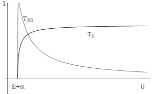
Figure 7: $T^{\rm rect\,step}_{\rm D}$ and $T^{\rm rect\,step}_{\rm KG}$ for $E=1.2\,m$ as functions of $U$ in the Klein zone

The situation is summarized in Fig. 7. The comparison of the two cases is self evident. Whereas, in the first case, the barrier is transparent for essentially all the values of the potential, in the second one, apart from a region just above the threshold of the Klein zone, the barrier becomes again impenetrable. This shows how wrong is the naive idea that only the oscillatory behaviour of the eigenfunction - due to the relativistic energy-momentum relation (3) - does all the job in the Klein zone. Indeed the equation for the large component of the Dirac equation (obtained by taking the derivative of the first equation in (16) and there using the second) is not equivalent to the Klein-Gordon equation (14). The derivative, acting on $U(x)$, yields extra terms $e\,{\cal E}=-U^{\prime}(x)$, thus supporting the expectation that a sharp edge is fundamental in making the difference between the previous results. This is indeed the content of Sauter’s work SA .

At this stage we can no longer help interpreting the scattering states. Indeed, in the scattering state identified by choosing $\gamma=0$ in (18), the positive (i.e. toward the right) current in the region $x>0$ cannot come from electrons with negative kinetic energy, see (6). It is rather due to positrons propagating backward in time, see viceversa (7). Hence - in the language of second quantization - a physical positron above the potential $-U$ comes from the right, i.e the $\delta$ term acts as a source of positrons available at $x=+\infty$. In this sense we are, therefore, in the presence of a $e^{+}$-$e^{-}$ annihilation process, and the reflection coefficient $R=1-T$ necessarily is smaller than 1. Had we had alternatively chosen $\delta=0$ in (18), we would have had, also from the right, an incoming current with an ensuing reflection coefficient bigger than 1. This would correspond to a flux of positrons travelling to the right, i.e. a process of pair creation. And this is the result much quoted as the ‘Klein paradox’, a statement that simply is not present in the original Klein’s paper. Let us however again stress that even for $R<1$ there is a paradox due to a finite fermion transmission through a high repulsive potential. Analogous considerations apply in the Klein-Gordon case with the previous provisions (Eq.s (28) and (30) and Fig. 7) due to the reversed role of the $\gamma$ and $\delta$ terms.

III Barriers

The space-inversion invariant potential barrier obtained by using twice the step (17) is

$$W(x)=U\big{(}x+\ell+L\big{)}+U\big{(}-(x+\ell+L)\big{)}$$ (36)

and the corresponding stationary states have the form

$$\Psi_{E}(x)=\begin{cases}\alpha\,u(p)\,e^{i\,p\,x}+\beta\,u(-p)\,e^{-i\,p\,x}&x<-(\ell+L)\\ \Xi_{-}(x)&-(\ell+L)<x<-L\\ \gamma\,u(q)\,e^{i\,q\,x}+\delta\,u(-q)\,e^{-i\,q\,x}&-L<x<L\\ \Xi_{+}(x)&L<x<\ell+L\\ \alpha^{\prime}\,u(p)\,e^{i\,p\,x}+\beta^{\prime}\,u(-p)\,e^{-i\,p\,x}&x>\ell+L\end{cases}$$ (37)

(the coefficients $\alpha,\,\beta,\,\gamma,\,\delta$ appearing in the latter equation should not be confused with those appearing in (18) to which they are however related through the translation $x\to x+\ell+L$). Again, the continuity relations at $x=-(\ell+L),\,-L$ and $x=L,\,\ell+L$ respectively entail

$$\begin{pmatrix}\gamma\\ \delta\end{pmatrix}=M^{\rm left}\,\begin{pmatrix}\alpha\\ \beta\end{pmatrix}\,,\qquad\begin{pmatrix}\alpha^{\prime}\\ \beta^{\prime}\end{pmatrix}=M^{\rm right}\,\begin{pmatrix}\gamma\\ \delta\end{pmatrix}$$ (38)

whence the transfer matrix relative to the barrier

$$\begin{pmatrix}\alpha^{\prime}\\ \beta^{\prime}\end{pmatrix}\equiv M^{\rm bar}\begin{pmatrix}\alpha\\ \beta\end{pmatrix}=\begin{pmatrix}A&B\\ B^{*}&A^{*}\end{pmatrix}\begin{pmatrix}\alpha\\ \beta\end{pmatrix}$$ (39)

is obtained as

$$M^{\rm bar}=M^{\rm right}M^{\rm left}\ .$$ (40)

The connection of $M^{\rm right}$ and $M^{\rm left}$ with $M^{\rm step}$ is established by taking translations and reflection into account. The effect of the translation to the left $x\to x+\ell+L$ is expressed with the aid of the matrix

$$T(k,a)=\begin{pmatrix}e^{i\,k\,a}&0\\ 0&e^{-i\,k\,a}\end{pmatrix}\cdot$$ (41)

One gets

$$M^{\rm left}=T(q,\ell+L)\,M^{\rm step}\,T(-p,\ell+L)$$ (42)

whereas $M^{\rm right}$ is obtained either by reflecting $x\to-x$ in $M^{\rm left}$, or by first reflecting $M^{\rm step}$ and then translating to the right $x\to x-(\ell+L)$:

$$M^{\rm right}=\sigma_{1}\,(M^{\rm left})^{-1}\,\sigma_{1}=$$

$$T\big{(}p,-(\ell+L)\big{)}\,\sigma_{1}(M^{\rm step})^{-1}\sigma_{1}\,T\big{(}-q,-(\ell+L)\big{)}\,.$$ (43)

Exploiting (40)-(43) one finally obtains for the coefficients appearing in (39)

$$A={a^{2}\,e^{2i(q-p)(\ell+L)}-b^{*\,2}\,e^{-2i(q+p)(\ell+L)}\over|a|^{2}-|b|^{2}}$$ (44)

$$B={a\,b\,e^{2iq\,(\ell+L)}-a^{*}\,b^{*}\,e^{-2iq\,(\ell+L)}\over|a|^{2}-|b|^{2}}\cdot$$ (45)

In the case of the barrier we do not have the ambiguity - connected with the identification of the scattering states - we have discussed for the step in (28) and (29). The transmission coefficient of the barrier is $1/|A|^{2}$ both in the Klein-Gordon and the Dirac case. When it is expressed in terms of the two matrix elements entering the transfer matrix of the step

$$a=|a|\,e^{i\,\xi}\,,\quad b=|b|\,e^{i\,\eta}\,,$$ (46)

takes the form

$$T^{\rm bar}\!=\!\frac{1}{1+\displaystyle{\frac{4|a|^{2}|b|^{2}}{(|a|^{2}\!-\!|b|^{2})^{2}}\sin^{2}\!\big{(}2q\,(\ell+L)+\xi+\eta\big{)}}}\cdot$$ (47)

This can be further simplified on account of (27)-(29):

$$T^{\rm bar}\!=\!\frac{1}{1+4\,\displaystyle{\frac{1-T^{\rm step}}{(T^{\rm step})^{2}}\,\sin^{2}\big{(}2q\,(\ell+L)+\xi+\eta\big{)}}}\cdot$$ (48)

The above formula is consistent with the results cited in the introduction, i.e. when (28)-(31) - appropriate for the rectangular barriers - are used, (8), (9) are reobtained.

The dependence of $T^{\rm bar}$ on the energy is through the phases $\xi$, $\eta$ of the transfer matrix elements (46), as well as through $T^{\rm step}$ itself and $q$. The dependence on the barrier width $2L$ is, instead, completely spelled out in the argument of the $\sin$ function. This means that for given energy, no matter how opaque the step ${\cal U}(x)$ may be, the width parameter $L$ can be always adjusted in such a way that the corresponding even barrier is totally transparent (this is analogue to the situation of dielectric stratified media in optics: see e.g. BW , where however only the case of sharp edge $\ell=0$, i.e. $\xi=\eta=0$, is considered). Going back to particles, as discussed in the introduction, there may be the difficulty that, for given average energy $\overline{E}$ and energy uncertainty $\Delta E$ of the incident particles, any ‘realistic’ value of $L$ may be such that too many maxima of $T^{\rm bar}$, due to the oscillations of $\sin^{2}(\dots)$, come into the range ($\overline{E}-{1\over 2}\Delta E,\overline{E}+{1\over 2}\Delta E$). The averaging procedure $\sin^{2}(\dots)\to{1\over 2}$ in (48) is then necessary and (12) follows immediately when $T^{\rm step}\ll 1$.

IV Sauter trapezoidal Barrier for the Dirac case

The analytic expression for $T^{\rm Sauter\ bar}_{\rm D}$ can be deduced from the long formulae we have extracted from Sauter’s paper SA and reported in the Appendix. The graphs below are more eloquent than the expression. In assigning numerical values to the parameters, we have in mind the case of electrons in vacuum. Therefore the unit of energy is $m=.51$ MeV and the unit of lenght is $\lambda_{\rm Compton}=.024$ Å.

We repeat here the warning already made in the Introduction: there may be cases where the units change by orders of magnitude and the following discussion may not apply.

In consequence of the scales we have chosen, the values we give to $U$ are not much higher than the threshold, typically $U=3\,m$. As for $\ell$ and $L$, certainly they both have to take a value of the order of at least $10^{2}\,\lambda_{\rm Compton}$. It is however instructive to vary one parameter at a time.

Figure 8: $T^{\rm Saut\,bar}_{\rm D}$ for $U=3\,m,\ L=0,\ \ell=3\,\lambda_{\rm Compton}$ as function of $E$ in the Klein zone

Fig. 8 plots $T^{\rm Saut\,bar}_{\rm D}$ against the energy $E$ in the Klein zone for $U=3m$, $\ell=3\lambda_{\rm Compton}$ and $L=0$: it is a triangular barrier that shows the effect of $\ell$ alone. It indicates that a flux of monoenergetic electrons ($\Delta E\ll$ width of the peak) is entirely transmitted. This may come a little bit as a surprise because, referring to Fig. 2 and in a pictorial space-time description, the incoming electron encounters:

(i) a free propagation region (from $x=-\infty$ to $x=0$);

(ii) a region from $0$ to $x_{1}$ that is still classically accessible, but where the propagation is non-free: the two solutions behave as (think e.g. of the semiclassical approximation) exponentials of opposite imaginary arguments;

(iii) the classically inaccessible region $(x_{1},x_{2})$ with non-propagating solutions: the two solutions of the Dirac equation behave as exponentials of opposite real arguments (a region that we will improperly call the ‘attenuation’ region);

(iv) eventually the classically inaccessible region from $x_{2}$ to $\ell$ where propagation, albeit non-free, still occurrs;

then, from $\ell$ to $+\infty$, the same steps just described, but in reverse order.

If one takes the Schrödinger case as a guidance, one might expect attenuation of the wave function both in the left and in the right attenuation region. This happens for almost all the values of $E$ in the Klein-zone, with the exception of the peak displayed. Indeed, for average energy $\overline{E}$ at the center of the peak, the single monocromatic components, that make up the incident packet, undergo two transmissions at the edges and possible multiple reflections in between, but they succeed in keeping somehow memory of the relative phases and the packet is (almost entirely) reconstructed beyond the barrier. For the values we have indicated the ‘device’ could serve as a monocromator for incident wave packets with energy uncertainty greater than the width of the displayed peak. From a practical point of view this is illusory, due to the exceedingly small value of $\ell=3\lambda_{\rm Compton}=0.072$ Å.

Fig. 9 shows the impact of increasing $L$ from 0 to $100\,\lambda_{\rm Compton}=2.4\,$ Åin the preceding case. A region of strict free propagation is interposed, the peak of Fig. 8 is replicated several times (the argument of the $\sin^{2}(\dots)$ in (48) oscillates much faster) and the peaks displayed all reach the value 1. However we have chosen to reduce the scale of the ordinates to make the energy averaged $\overline{T}^{\rm Saut\,bar}_{\rm D}$ visible. The oscillations of the non-averaged $T$ are so fast (and still the value given to $L$ may be largely considered too small) that only $\overline{T}$ is susceptible of comparison with the data of whatever ‘Gedanken’ experiment. Nonetheless a value of $\overline{T}$ of the order of some part per thousand could still be considered an interesting signal.

Figure 9: $T^{\rm Saut\,bar}_{\rm D}$ for $U=3\,m,\ L=100\,\lambda_{\rm Compton},\ell=$ $3\,\lambda_{\rm Compton}$ as function of $E$ in the Klein zone

Once the role of $L$ is understood, in Fig. 10 we go back to the case $L=0$ but raise the value of $\ell$ from $3\,\lambda_{\rm Compton}$ to $100\,\lambda_{\rm Compton}$. The main difference is in the scale of the ordinates. Again the peaks all reach the value 1, but the scale of $\overline{T}$ has dropped to $10^{-90\div 91}$. As for the part of the Klein zone that also satisfies $E-m\simeq m$, this is in perfect agreement with (12)).

The analytical result, displayed in the figure, shows that the estimate extends to the whole Klein zone.

The number of peaks in the Klein zone increases with increasing $\ell$, but the width of each of them shrinks much faster: this is why the value of $\overline{T}$ has dropped of so many orders of magnitude.

Figure 10: $T^{\rm Saut\,bar}_{\rm D}$ for $U=3\,m,\ L=0,\ \ell=100\,\lambda_{\rm Compton}$ as function of $E$ in the Klein zone

Turning $L$ on will not appreciably change the scale of the ordinates, but the energy averaging becomes unavoidable. This washes out any phase information among the monoenergetic components the incident packet is made of. As a consequence the packet, that has undergone an attenuation in the attenuation region at the first edge, may only undergo a second attenuation at the second edge. The result is that the transmission coefficient (48) is shattered down to the asymptotic value given in (12).

Finally the trapezoidal form of the barrier, we have chosen in order to be able to exhibit analytical results, should not be crucial to the above conclusion. The same qualitative result should obtain with all the barriers where the dimension $\ell$ of the regions that support a relevant electric field ($e\,{\cal E}>2m^{2})$ is large enough so as to fulfill (5). Ref. Z2 , where again Sauter provides analytical results for the potential

$$U_{1}(x)={U\over 2}\left(1+\tanh{x\over\ell}\right)$$

as well as the relevant asymptotics, substantiates the above expectation.

The foregoing argument should also work for the ‘delocalization’ of particles in supercritical potentials GZ , GZG . This will be possibly considered elsewhere.

Appendix A Linearly raising potential and Sauter solution for the Dirac Case

Referring to the Dirac equation with the step potential of Fig. 2

$${\cal U}(x)=U\,{x\over\ell}\ \,,\qquad 0\leq x\leq\ell$$ (49)

the solution $\Xi(x)$ in the intermediate region $0<x<\ell$ to be fed in (18) can be worked out from Sauter’s article SA . His representation for the Dirac Hamiltonian is different from Pauli’s (15): he uses

$$H_{\rm D}^{\rm Sauter}=i\,\sigma_{3}\frac{d}{dx}+U(x)-\sigma_{2}\,m=V\,H_{\rm D}^{\rm Pauli}\,V^{\dagger}$$ (50)

with (up to an irrelevant phase factor)

$$V=\frac{1}{2}\big{(}I-i\,(\sigma_{1}+\sigma_{2}-\sigma_{3})\big{)}\ .$$ (51)

He then introduces the argument

$$\xi(x)=\sqrt{\frac{U}{\ell}}\Big{(}x-{E\over U}\,\ell\Big{)}$$ (52)

and the degenerate hypergeometric function

$$\Phi(\alpha,\beta;z)=1+\frac{\alpha}{\beta}\,\frac{z}{1!}+\frac{\alpha(\alpha+1)}{\beta(\beta+1)}\,\frac{z^{2}}{2!}+\dots$$ (53)

in terms of which the two independent eigenfunctions belonging to energy $E$

$$\Sigma=\begin{pmatrix}f_{E}(x)\\ g_{E}(x)\end{pmatrix}\,,\quad\widetilde{\Sigma}={\cal C}\Sigma=\sigma_{1}\Sigma^{*}=\begin{pmatrix}g_{E}^{*}(x)\\ f_{E}^{*}(x)\end{pmatrix}$$ (54)

in the intermediate region $0<x<\ell$ are given by

$$f_{E}(x) =e^{i\,\xi^{2}/2}\,\Phi\left(\frac{i}{4}\,\frac{m^{2}\,\ell}{U},\frac{1}{2},-i\,\xi^{2}\right)$$ (55)

$$g_{E}(x) =-m\,\sqrt{\frac{\ell}{U}}\,e^{i\,\xi^{2}/2}\,\Phi\left(\frac{i}{4}\,\frac{m^{2}\,\ell}{U}+1,\frac{3}{2},-i\,\xi^{2}\right).$$ (56)

Thanks to (51), the $\Xi(x)$ to be fed in (18) is the linear combination

$$\mu\begin{pmatrix}f_{E}(x)+ig_{E}(x)\\ -f_{E}(x)+ig_{E}(x)\end{pmatrix}+\nu\,\begin{pmatrix}g_{E}^{*}(x)+if_{E}^{*}(x)\\ -g_{E}^{*}(x)+if_{E}(x)\end{pmatrix}\,.$$ (57)

The transfer matrix $M^{\rm Saut\ step}_{\rm D}$ is obtained by imposing the continuity of (18) at $x=0$ and $x=\ell$ and then eliminating $\mu$ and $\nu$. Its matrix elements (23) turn out to be

$$a^{\rm Saut\ step} =\frac{e^{-i\,q\,\ell}}{4q\,(E+m)}\ \Big{(}P_{+}Q_{+}R-P_{-}Q_{-}R^{*}+i\,\big{(}P_{+}Q_{-}S+P_{-}Q_{+}S^{*}\big{)}\Big{)}$$ (58)

$$b^{\rm Saut\ step} =\frac{e^{-i\,q\,\ell}}{4q\,(E+m)}\ \Big{(}P_{-}Q_{+}R-P_{+}Q_{-}R^{*}+i\,\big{(}P_{-}Q_{-}S+P_{+}Q_{+}S^{*}\big{)}\Big{)}$$ (59)

where

$$R =f_{E}^{\phantom{*}}(0)\,f_{E}^{*}(\ell)-g_{E}^{*}(0)\,g^{\phantom{*}}_{E}(\ell)$$ (60)

$$S =f_{E}^{\phantom{*}}(0)\,g_{E}^{*}(\ell)-g_{E}^{\phantom{*}}(0)\,f^{*}_{E}(\ell)$$ (61)

$$P_{\pm} =E+m\pm p$$ (62)

$$Q_{\pm} =E-U+m\pm q\ .$$ (63)

Substitution of the above formulae in (46)-(48) provides the analytic expression for $T^{\rm Saut\ step}_{\rm D}$ by which the graphs of Fig.s 8-10 above are obtained. Finally Sauter himself works out the asymptotic form (4) that $T^{\rm Saut\ step}_{\rm D}$ has when both $E-m\simeq m$ and (5) are satisfied:

$$T^{\rm Saut\ step}_{\rm D}={q\,(U-E+q)\over p\,(E+p)}\,e^{-\pi\,m^{2}\ell/U}\,\big{(}1+{\cal O}(U/m^{2}\ell)\big{)}$$

having included a prefactor omitted in (12).

References

- (1) Klein O., Z. Phys. 53, 157 (1929)
- (2) Calogeracos A., Dombey N., Contemp. Phys. 40, 313 (1999)
- (3) Sauter F., Z. Phys. 69, 742 (1931)
- (4) Krekora P., Su Q., Grobe R., Phys. Rev. Lett 92, 040406 (2004)
- (5) De Leo S., Rotelli P. P., Phys. Rev. A, 73, 42107 (2006)
- (6) Katnelson M. I., Novoselov K. S., Geim A. K., Nature Phys. 2, 620 (2006)
- (7) Calogeracos A., Nature (Physics) 2, 579 (2006)
- (8) Bjorken J. D., Drell S. D., Relativistic Quantum Mechanics, (McGraw-Hill, New York, 1964)
- (9) Born M., Wolf E., Principles of Optics, (Pergmon Press, Oxford UK, 1986)
- (10) Sauter F., Z. Phys. 73, 547 (1931)
- (11) Gerstein S. S., Zel’dovich Ya. B., Sov. Phys. JETP 30, 358 (1970)
- (12) Greiner W. in Quantum Electrodynamics of Strong Fields, Greiner W. (Ed.), NATO ASI Series vol. 80 (Plenum Press, N.Y. 1983)