Phase rigidity breaking in open Aharonov-Bohm ring coupled to a cantilever

Abstract

The conductance and the transmittance phase shifts of a two-terminal Aharonov-Bohm (AB) ring are analyzed in the presence of mechanical displacements due to coupling to an external cantilever. We show that phase rigidity is broken, even in the linear response regime, by means of inelastic scattering due to phonons. Our device provides a way of observing continuous variation of the transmission phase through a two-terminal nano-electro-mechanical system (NEMS). We also propose measurements of phase shifts as a way to determine the strength of the electron-phonon coupling in NEMS.

Nanoelectromechanical systems (NEMS) have been a subject of extensive research in recent years. The possibility of combining electrical and mechanical degrees of freedom on the nanoscale may give rise to technological advantages as well as manifestations of fundamental physical phenomena. From a technological point of view the interest is largely due to the many applications that may be realized using NEMS.cleland_review_NEM It follows ubiquitously from the concrete possibility of downsizing devices from micromechanical into nanoelectromechanical systems. Among the many NEMS phenomena of considerable physical interest, we focus in this paper on the effect of quantum-coherent displacements in the presence of a Aharonov-Bohm effect in a one-dimensional ring symmetrically connected to two external leads. On the nanoscale level the mechanical forces controlling the structure of the system are of the same order of magnitude as the capacitive electrostatic forces governed by charge distributions. This circumstance is of the utmost importance when analyzing electron tunneling. For example, some predictions on the role of electron-phonon interactions on the electron tunneling have regarded the modifications of the peak-to-valley current ratio due to inelastic processes with important consequences in device applicationsgoldman_dephasing ; dephasing_cond . Another important issue in NEMS physics is related to the way mechanical displacements perturb phase coherent charge transport through closed loops as a consequence of the shifting of electron trajectories. For example, important information come from the Aharonov-Bohm (AB) oscillations in mesoscopic ringsyacoby_AB ; buks_AB ; stern_AB ; yeyati_AB ; feng_AB . Here, the loss of coherence, or dephasing, due to inelastic scattering caused by phonons reveals in the suppression of $hc/e$ oscillations. Another important aspect unnoticed in previous studies of NEMS is that inelastic scattering breaks phase-rigidity, i.e. the linear conductance is not symmetric in the AB phase. Here we show that the observed asymmetry can be tuned continuously by changing the electron-phonon coupling, demonstrating that the phase of the linear conductance in a two-terminal AB interferometer is not rigid when tunneling is assisted by phonons. The problem of phase rigidity and its breaking in ring and ring-dot systems has been largely investigated both theoreticallyimry_review ; jayannavar ; yeyati_AB ; phase_rig_1 ; phase_rig_2 ; phase_rig_3 ; sun99 and experimentallybuks_exp ; exp_kobayashi1 ; exp_kobayashi2 ; leturcq06exp . Here we address for the first time the problem in the framework of nanoelectromechanical systems and propose a way to detect phase rigidity breaking.

We consider a one-dimensional ring symmetrically coupled to two leads and to a mechanical cantilever. A coupling between the electrons travelling in the lower arm of the ring and the cantilever, whose tip is suspended over the arm, can be set up by developing a uniform electric field between the tip, the cantilever and the lower arm. Electrons couple approximately linearly to the cantilever position, thus leading to a coupling between the flexural phonon modes of the cantilever and the local density of the electrons on the ring arm. Furthermore, because the coupling strength decays rapidly with increasing frequency, for micron scale cantilevers only the fundamental flexural mode is relevant. Therefore, at low enough temperature, the cantilever can be treated as a single quantum mechanical oscillator. Of course the dephasing behavior of the electrons due to the cantilever depends on the relative magnitudes of the electron dwell time on the lower arm of the ring and the cantilever period. A similar device has been proposed by A. MacKinnon and A. D. Armour as a which-path device for electrons [armour03, ].

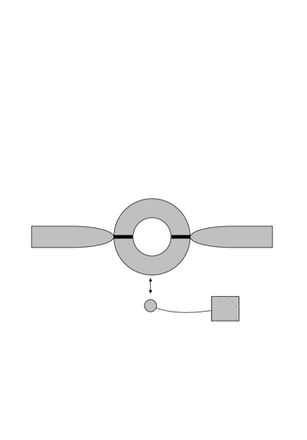
Figure 1: Device: A mesoscopic ring symmetrically coupled to two external leads and a cantilever.

In the following we generalize the scattering matrix approach in a way suitable for electron dwell times shorter or comparable to the cantilever period. In this way both elastic and inelastic contributions to the scattering process will appear. The Hamiltonian of the system shown in Fig.1 is written as:

$$\mathcal{H}=\mathcal{H}_{r}+\mathcal{H}_{c}+\mathcal{H}_{int},$$ (1)

where $\mathcal{H}_{r}$ and $\mathcal{H}_{c}$ are the Hamiltonian of the ring (in polar coordinates) and the cantilever, respectively:

$$\mathcal{H}_{r}=\frac{\hbar^{2}}{2m_{e}R^{2}}\left(-i\frac{\partial}{\partial\varphi}-\frac{\Phi_{AB}}{\phi_{0}}\right)^{2}$$ (2)

$$\mathcal{H}_{c}=\frac{p^{2}_{y}}{2M_{c}}+\frac{M_{c}\omega^{2}y^{2}}{2},$$ (3)

while $\mathcal{H}_{int}$ describes the interaction between the lower arm of the ring ($0<\varphi<\pi$) and the cantilever

$$\mathcal{H}_{int}(x=R\varphi,y)=\begin{cases}\alpha y&\text{$0<\varphi<\pi$},\\ 0&\text{otherwise},\end{cases}$$ (4)

where $\alpha$ represents the average of the electron density on the lower arm of the ring times the uniform electric field. The interaction between the electrons on the lower arm of the ring and the cantilever is modelled as a linear coupling between the displacement of the flexural mode and the average electron density of the lower arm of the ring, since when electrons are not in the ring there is no displacement of the cantilever (we assume that all positions are measured from the equilibrium height of the cantilever). The linear coupling is a valid approximation in the limit in which the displacement of the cantilever from its equilibrium height is small compared to the characteristic length of the harmonic oscillator. The Hamiltonian of left and right lead is given by the free particle Hamiltonian $\mathcal{H}_{lead}=-\hbar^{2}\partial^{2}_{x^{2}}/(2m_{e})$. By combining the harmonic potential of the cantilever with the interaction term $\mathcal{H}_{int}$, the effective potential along the lower arm can be rewritten as:

$$V_{eff}=\frac{1}{2}M_{c}\omega^{2}(y+\frac{\alpha}{M_{c}\omega^{2}})^{2}-\frac{\alpha^{2}}{2M_{c}\omega^{2}}.$$ (5)

In the following we solve the scattering problem, generalized to include inelastic scattering as in Ref.bonca99, . For our purposes, we set up a scattering problem by following the method of quantum waveguide transport on networksxia_waveguide ; deo_94 . One main problem is the boundary conditions at the intersection with the external leads. In this case the Griffith boundary’s conditiongriffith_boundary state that (i) the wave function must be continuous and (ii) the current density must be conserved. We assume that when an electron moves along the upper arm in the clockwise direction from $\varphi=0$, it acquires a phase $\Phi_{AB}/2$ at the output intersection $\varphi=\pi$, whereas the electron acquires a phase $-\Phi_{AB}/2$ in the counterclockwise direction along the lower arm when moving from $\varphi=0$ to $\varphi=\pi$. The wave-function for the right (out) /left (in) lead and the upper (up)/lower (low) arm of the ring may be written as:

$$\psi_{in}(x,y)=\phi_{l}(y)e^{ikx}+\sum^{\infty}_{m=0}r_{ml}\phi_{m}(y)e^{-ik_{m}x}$$ (6)

$$\psi_{out}(x,y)=\sum^{\infty}_{m=0}t_{ml}\phi_{m}(y)e^{ik_{m}x}$$ (7)

$$\psi_{up}(x,y)=\sum^{\infty}_{m=0}\phi_{m}(y)(a_{ml}e^{ik^{+}_{m}x}+b_{ml}e^{-i\pi f}e^{-ik^{-}_{m}x})$$ (8)

$$\psi_{low}(x,y)=\sum^{\infty}_{m=0}\phi_{m}(y+y_{0})(A_{ml}e^{i\tilde{k}^{-}_{m}x}+B_{ml}e^{i\pi f}e^{-i\tilde{k}^{+}_{m}x}),$$ (9)

where $\phi_{n}(y)$ represents the $n-$phonon state, and we have defined $f=\frac{\phi_{AB}}{\phi_{0}}$. The electron wavevectors, determined by the energy conservation, are $k_{m}=\sqrt{k^{2}+p^{2}(l-m)}$, $\tilde{k}_{m}=\sqrt{k^{2}+p^{2}(l-m+\gamma^{2})}$, $p^{2}=2m_{e}\omega/\hbar$, $k^{\pm}_{m}=k_{m}\pm\pi f/L$, $\tilde{k}^{\pm}_{m}=\tilde{k}_{m}\pm\pi f/L$ ($L=\pi R$ being the half circumference). The phonon wave function in the lower arm is shifted of the quantity $y_{0}=\frac{\alpha}{M_{c}\omega^{2}}$ and we have defined the dimensionless parameter $\gamma=y_{0}\sqrt{\frac{M_{c}\omega}{2\hbar}}$. The unknown transmission and reflection coefficients are determined by solving the following system of equations corresponding to the Griffith’s boundary conditions:

$$\psi_{in}(0,y)=\psi_{up}(0,y)=\psi_{down}(0,y)$$

$$\psi_{out}(\pi R,y)=\psi_{up}(\pi R,y)=\psi_{down}(\pi R,y)$$

$$\partial_{x}\psi_{up}(x=0,y)+\partial_{x}\psi_{down}(x=0,y)=\partial_{x}\psi_{in}(x=0,y)$$

$$\partial_{x}\psi_{out}(x=\pi R,y)-\partial_{x}\psi_{up}(x=\pi R,y)=\partial_{x}\psi_{down}(x=\pi R,y).$$ (10)

To eliminate the dependence on $y$, we project each equations on the phonon state $\phi_{s}(y)$, the only non-trivial projection being $\int^{\infty}_{-\infty}\phi_{s}(y)^{\ast}\phi_{m}(y+y_{0})dy$. Since $y_{0}$ is small quantity we may expand $\phi_{m}(y+y_{0})$ as $\phi_{m}(y+y_{0})\approx\phi_{m}(y)+\gamma(\sqrt{m}\phi_{m-1}(y)-\sqrt{m+1}\phi_{m+1}(y))$, which allows immediately to get the following result:

$$\int^{\infty}_{-\infty}\phi_{s}(y)^{\ast}\phi_{m}(y+y_{0})dy\approx\delta_{s,m}+\gamma(\sqrt{m}\delta_{s,m-1}-\sqrt{m+1}\delta_{s,m+1}).$$ (11)

Since $\gamma$ is a small quantity, only one-phonon processes are relevant and the scattering problem can be solved with arbitrary numerical accuracy.

In order to solve the linear system (Phase rigidity breaking in open Aharonov-Bohm ring coupled to a cantilever) for the unknown transmission and reflection coefficients, a pruning procedure has been applied (similar to Ref.bonca99, ). The method is based on the simple idea of fixing the number of phonon modes at $s=S$, and than iteratively removing all the coefficients with phonon indices greater than $S$, adjusting the remaining transmission and reflections coefficients in such a way to have a total probability (reflection and transmission) equal to one. Once fixed $s=S$, the problem reduces to solve a linear system in the variables $r_{sl},t_{sl},a_{sl},b_{sl},A_{sl},B_{sl}$, with $s=0,\ldots,S$. In the following we consider $S=4$. Once the scattering problem is solved, the transmission probability, both for elastic and non-elastic processes, is defined as follows:

$$\mathcal{T}_{ml}=|t_{ml}|^{2}\frac{k_{m}}{k_{l}},$$ (12)

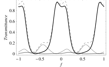
Figure 2: Transmissions coefficients $\mathcal{T}_{11}$ (thick black line), $\mathcal{T}_{21}$ (full line), and $\mathcal{T}_{01}$ (thick grey line) as a function of the Aharonov-Bohm flux $f$ with the following choice of parameters: $kL=3.5$, $\gamma=0.2$, $pL=3$. The dashed curve represents the total transmission including also 3 and 4 phonons contribution.

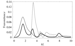
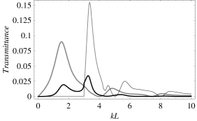
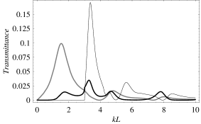
Figure 3: Transmissions coefficients $\mathcal{T}_{11}$(thick black line), $\mathcal{T}_{21}$ (full line), and $\mathcal{T}_{01}$ (thick grey line) as a function of $kL$ for the following choice of parameters: $\gamma=0.2$, $pL=3$ and $f=0.49,0.5,0.51$(top to bottom).

where $\mathcal{T}_{ml}$ represents the transmission probability from the $l$-phonon state to the $m$-phonon state. In what follows we assume that the starting phonon state is $l=1$, and the initial electron momentum $k_{l}$ is fixed to $k$. The total transmission probability is obtained as $\sum_{m}\mathcal{T}_{m1}$. We solved the scattering problem for $s=0,1,2,3,4$ phonons, assuming the initial state of the cantilever corresponding to the single phonon state ($l=1$). In Fig.2, the transmission coefficients and the transmittance are shown as a function of the external flux $f$ for $kL=3.5$, $\gamma=0.2$ and $pL=3$. Even tough the main contribution to the transmission is generally due to the elastic term $t_{11}$, a strong influence of the inelastic term $t_{21}$ is observed close to half-integer values of the flux. The lifting from zero of the conductance close to an half-integer flux is the signature of a phonon-assisted tunnelling (PAT). To better discern elastic from inelastic contributions to the scattering in Fig.3 the transmission coefficients $t_{11},t_{21},t_{01}$ are plotted as a function of $kL$ for $\gamma=0.2$, $pL=3$ and $f=0.49,0.5,0.51$ (from top to bottom). As above, a strong competition between elastic and inelastic scattering amplitudes is observed close to half-integer values of the flux. A general feature of all the panels in Fig.3 is that in the low energy region ($kL<3$) the scattering amplitude is dominated by the coefficient $t_{01}$ describing the process of emission of a phonon. In the intermediate energy region ($3<kL<5$) the transmission appears strongly affected by a resonant peak related to absorption of a phonon ($t_{21}$), while in the high energy region ($kL>5$) an alternating behavior is observed. Further, in Fig.3(top panel), close to $kL=4$, only the inelastic coefficient $t_{21}$ contributes to the transmission. This follows from the fact that an electron can be transmitted only by changing the cantilever state, i.e. by means of the absorption/emission of a phonon in the final state. Similar behavior can be seen for other initial momenta $kL$.

Let us apply the general conductance formula in the linear response regime (Landauer-Büttiker formulalandauer_cond ), to investigate the dependence of the transmission on the flux $\phi$ and through that obtain the behavior of the phase shift. The transmission phase through a mesoscopic AB ring has the general property of phase rigidity coming from the two-terminal nature of the set-up and which is generally based on time-reversal symmetry-breaking and current conservationbuttiker_prl_86 , i.e. the transmission probability amplitude satisfies the property $\mathcal{T}_{\alpha\beta}(kL,\phi)=\mathcal{T}_{\beta\alpha}(kL,-\phi)$ as a function of the flux and of the incident electron energy ($\alpha,\beta=L,R$ being the lead index). Combining time-reversal symmetry requirement with current conservation $|\mathcal{T}_{\alpha\beta}(kL,\phi)|^{2}=|\mathcal{T}_{\beta\alpha}(kL,\phi)|^{2}$, implies that the linear conductance $\mathcal{G}$ is an even function of the flux, whose Fourier transform is

$$\mathcal{G}(\phi)=\mathcal{G}_{0}+\sum_{n}\mathcal{G}_{n}\cos(n\phi+\delta_{n}),$$ (13)

and $\phi=2\pi f$. Obviously, the phase shift $\delta_{n}$ can take only two values $0$ and $\pi$note_hilbert_transf . Thus, the phase of the two terminal AB ring has to be rigid, or change abruptly by $\pi$ as the accumulated phase in one arm is being varied. This peculiar behavior, known as phase rigidity has been studied extensivelyimry_review ; buks_exp ; yeyati_AB ; phase_rig_1 ; phase_rig_2 ; phase_rig_3 ; sun99 ; leturcq06exp . Experimentallybuks_exp ; exp_kobayashi1 ; exp_kobayashi2 and theoreticallyjayannavar various methods of avoiding phase-rigidity in rings and ring-dots systems were previously discussed. Here we are proposing, for the first time, observation of phase rigidity breaking in a nanoelectromechanical system as an alternative way of observing the continuous variation of the transmission phase through a two-terminal mesoscopic system. Our results in Fig.4 show that for different values of the interaction $\gamma$ inclusion of inelastic scattering, breaks phase rigiditynote_onsager ; kang_onsager . The first evidence for this comes from the fact that $\mathcal{T}$ is non symmetric. This is clearly seen in the vicinity of the antiresonances in the conductance, which are approximately located at the energy values determined by the electron-phonon coupling $\gamma$:

$$K^{l}_{nm}L\approx\sqrt{\pi^{2}(n+f)^{2}+(pL)^{2}(l-m+\gamma^{2})},$$ (14)

where $n$ labels the momentum of the eigenstates in the ring, $m(l)$ labels the final(initial) phonon channel. The amount of phase rigidity violation depends on strength of $\gamma$ and it is related to the momentum of incoming electron. For instance, in Fig.4, the total transmission as a function of the flux $f$ is shown, for $pL=3$, $kL=5.5$ and varying $\gamma$ from zero to $0.2$ (from top to bottom with step 0.05). Since the phase shift is a measurable quantity in the experiments, in Figs.5, the behavior of $\delta_{1}$ is shown as a function of $\gamma$ for different values of the antiresonance momenta. As shown, in the absence of interaction, i.e. under Onsager symmetry, the phase shift is equal to $\pi$, corresponding to a local minimum in the conductance versus flux close to $f=0$. When the interaction is turned on, the phase shift $\delta_{1}$ converges quite rapidly to the values $\pi/2$ or $3\pi/2$, depending on the value of the momentum $kL$. The interaction region characterized by a rapid variation of the phase shift can be exploited in experiments to obtain information on the electron-phonon coupling simply by measuring the phase shift of the linear conductance. Furthermore, since this analysis can be done for all the antiresonances, the value of the interaction $\gamma$ can be obtained by experimental measurements of the phase shift. The phase rigidity breaking we have discussed, has close similarities to that described by Sun et al. in [sun99, ] where a two-terminal modified AB ring with a quantum dot inserted in one arm has been considered. There, the phase rigidity is broken in the linear regime by applying a time-varying microwave (MW) field on the quantum dot. Further, the behavior of the phase shift in Figs.5 is similar to that shown in Fig. 4 of Ref.leturcq06exp, for non-linear transport in an AB ring. Even tough, the experimental analysis as a function of a perpendicular magnetic field is focused on nonlinear contribution to the conductance, the analogy in the phase shift behavior can be associated to an effective energy shift in the lower arm provided in our case by the interaction with the cantilever, while there is due to a gate voltage.

In conclusion, we have analyzed the transmittance and the phase shifts behavior in a two-terminal AB ring whose lower arm is coupled to a cantilever. We showed that the phase rigidity can be broken as an effect of the inelastic scattering channels introduced by the cantilever, and a continuous phase shift can be obtained through the measurements of the linear conductance. The continuous phase variation as a function of the incident electron energy in experiments can be exploited to obtain the value of the electron-phonon coupling. Our proposal is within reach with today’s technology employed in nanoelectromechanical systems. It can be realized by means of a semiconducting ring (e. g. In As hui ) operating at mK temperatures with radius $R\approx 60\div 100nm$ coupled to a molecular cantilever (e. g. a cantilevered or bridged single walled carbon nanotube chunyu ) with a mass $\approx 10^{-24}\div 10^{-23}kg$ and with fundamental frequency $\omega\approx 10^{2}\div 10^{3}GHz$, thus allowing to realize dwell times for the electrons less or of the order of the cantilever frequency. The cantilever length can be taken of the order of the (0.02-0.05)$\mu$m and its distance from the arm of the ring of the order (0.01-0.1)$\mu$m. In this way an extra electron in correspondence of the position of the tip causes a small vertical displacement. The phase rigidity breaking can be regarded a common feature of two-terminal nanomechanical systems and thus we propose measurements of phase shifts as a way to determine the strength of the electron-phonon coupling in NEMS.

I Acknowledgments

We acknowledge Fabio Pistolesi for his enlightening comments and careful reading of the paper. F. Romeo thanks the laboratory LPMMC of Grenoble for kind hospitality.

Figure 4: Total transmission amplitude as a function of the total flux $f$. The curves correspond to the following choice of parameters: $kL=5.5$, $pL=3$ and $\gamma$ from $0$ to $0.2$ (top to bottom with step $0.05$).

Figure 5: Phase shift $\delta_{1}$ computed for: $kL=7$ (box) and $kL=5.5$ (diamond) [left panel] and $kL=8.9$ (box) and $kL=9.9$ (diamond) [right panel] by fixing $pL=3$. In all the curves $\delta_{1}=\pi$ when $\gamma=0$.

References

- (1) A.N. Cleland, Foundations of Nanomechanics, Springer- Verlag: Berlin, 2003.
- (2) V. J. Goldman, D. C. Tsui, and J. E. Cunningham, Phys. Rev. B 36, 7635 (1987).
- (3) L. P. Kouwenhoven, S. Jauhar, J. Orenstein, and P. L. McEuen, Phys. Rev. Lett. 73, 3443 (1994);
- (4) A. Yacoby, M. Heiblum, D. Mahalu and H. Shtrikman, Phys. Rev. Lett. 74, 4047 (1995).
- (5) E. Buks, R. Schuster, M. Heiblum, D. Mahalu, V. Umansky, and H. Shtrikman, Phys. Rev. Lett. 77, 4664 (1996).
- (6) A. Stern, Y. Aharonov, and Y. Imry, Phys. Rev. A 41, 3436 (1990).
- (7) A. L. Yeyati and M. B uttiker, Phys. Rev B, R14360 (1995).
- (8) Shechao Feng, Phys. Lett. A 143, 400 (1990).
- (9) Y. Imry, Introduction to Mesoscopic Physics, (Oxford University Press, Oxford, U.K.) (1997).
- (10) P. Singha Deo and A. M. Jayannavar, Mod. Phys. Lett. B10, 787 (1996).
- (11) G. Hackenbroich and H. A. Weidenmuller, Phys. Rev. Lett. 76, 110 (1996); Phys. Rev. B 53, 16 379 (1996).
- (12) A. Yacoby, R. Schuster, and M. Heiblum, Phys. Rev. B 53, 9583 (1996).
- (13) C. Bruder, R. Fazio, and H. Schoeller, Phys. Rev. Lett. 76, 114 (1996).
- (14) R. Englman and A. Yahalom, Phys. Rev. B 61, 2716 (2000).
- (15) Q. Sun, J. Wang and T. Lin, Phys. Rev. B 60, R13981 (1999).
- (16) E. Buks, R. Schuster, M. Heiblum, D. Mahalu and V. Umansky, Nature 391, 871 (1998).
- (17) K. Kobayashi, H. Aikawa, S. Katsumoto and Y. Iye, Phys. Rev. B 68, 235304 (2003)
- (18) K. Kobayashi, H. Aikawa, A. Sano, S. Katsumoto and Y. Iye, Phys. Rev. B 70, 035319 (2004)
- (19) R. Leturcq et al., Phys. Rev. Lett. 96, 126801 (2006).
- (20) A. MacKinnon and A. D. Armour, J. Phys. Soc. Jpn. 72, 118-122 (2003) Suppl.A and references therein.
- (21) K. Haule and J. Bonča, Phys. Rev. B 59, 13087 (1999).
- (22) J.B. Xia, Phys. Rev. B 45, 3593 (1992).
- (23) P. S. Deo and A. M. Jayannavar, Phys. Rev. B 50, 11 629 (1994).
- (24) S. Griffith, Trans. Faraday Soc. 49, 345 (1953).
- (25) R. Landauer, Philos. Mag. 21, 863 (1970).
- (26) M. Buttiker, Phys. Rev. Lett. 57, 1761 (1986).
- (27) The scattering phase-shift can also be determined by the Hilbert transform of the scattering probability as shown in Ref.[14].
- (28) The phase rigidity breaking is also connected to the violation of the Onsager rule (L. Onsager, Phys. Rev. 38, 2265 (1931); H.B. G. Casimir, Rev. Mod. Phys. 17, 343 (1945)). Under Onsager symmetry all the phase shift are constrained to be 0 or . In the case of a symmetry breaking such phases can vary continuously.
- (29) G. L. Khym and K. Kang, Phys. Rev. B 74, 153309 (2006).
- (30) Hui Hu et al., Phys. Rev. B 63, 045320 (2001).
- (31) Chunyu Li and Tsu-Wei Chou, Phys. Rev. B 68, 073405 (2003).