Solution of the Dirac Equation using the Lanczos Algorithm

Abstract

Covergent eigensolutions of the Dirac Equation for a relativistic electron in an external Coulomb potential are obtained using the Lanczos Algorithm. A tri-diagonal matrix representation of the Dirac Hamiltonian operator is constructed iteratively and diagonalized after each iteration step to form a sequence of convergent eigenvalue solutions. Any spurious solutions which arise from the presence of continuum states can easily be identified.

PACS 03.65.Ge, 02.60.Lj

I Introduction

In relativistic quantum mechanics, the calculation of the lowest lying bound states of a relativistic electron in a static Coulomb potential is a classic problem. In some respects the perturbative solution provided by BetheBethe (1964) is both simple and elegant and a standard example in many textbooks. Early attempts to obtain the exact eigensolutionsJ. P. Desclaux (1975); I. P. Grant et al. (1976) employed finite difference methods to solve the radial equations and obtain the eigenenergies. Recently much effort has focused on the extension of basis set methodsC. Krauthauser and R. Hill (2002); G. W. F. Drake and S. P. Goldman (1981); S. P. Goldman and G. W. F. Drake (1982, 1988) which have been applied with success in non-relativistic quantum mechanics. Such matrix approximations of the Dirac equation are usually obtained from a variational principle with the radial components approximated by a finite number of terms of a basis-set expansion. They often display pathological features such as the occurrence of unphysical spurious solutionsW. Kutzelnigg (1984); C. Krauthauser and R. Hill (2002) and a failure to vary systematically with the basis-set size. These can for the most part be avoided if a resolvent operator rather than the Dirac Hamiltonian is used in the variational principleC. Krauthauser and R. Hill (2002) or by construction in explicit finite basis-set calculationsS. P. Goldman (1985). Accurate numerical solutions have also recently been obtained using mapped Fourier grid methodsE. Ackad and M. Horbatsch (2005); J. P. Boyd et al. (2003). Spurious roots are still present in certain cases but can easily be identifiedE. Ackad and M. Horbatsch (2005).

For the Coulomb potential with a coupling constant which is less than $\sqrt{\frac{3}{2}}$, the Dirac Hamiltonian is self-adjoint in the first Sobolev spaceB. Thaller (1992). Hence, as we shall show, its eigenpairs can be obtained iteratively in an absolutely convergent manner by means of the Lanczos AlgorithmLanczos (1950); Kreuzer et al. (1981) provided, of course, that only the positive energy eigensolutions are considered. Although the Lanczos Algorithm is generally known for its application to conventional matrix eigenvalue problems, it can be used to solve eigenvalue problems of a self-adjoint operator which is bounded from below or aboveKreuzer et al. (1981). In the former case, the matrix to be diagonalized is iteratively transformed into a tri-diagonal matrix and diagonalized after each iteration step to form a sequence of convergent eigenvalue solutions. In the latter case, a tri-diagonal representation of the self-adjoint operator is constructed iteratively and diagonalized after each iteration step to form a sequence of convergent eigenvalue solutions. Any spurious solutions which arise from the presence of continuum states can easily be identified in manner recently suggestedAndrew and Miller (2003). Furthermore, many of the aforementioned problems are avoided if the following iterative scheme proposed by Lanczos is employed.

II The Lanczos Method

Given the following eigenvalue problem

$$\hat{H}|E_{\lambda}\rangle=E_{\lambda}|E_{\lambda}\rangle$$ (1)

where $\hat{H}$ is a self-adjoint operator (not necessarily bounded) in a separable Hilbert (or Sobolev) space which possesses a number of eigenvalues $E_{\lambda}$ (not necessarily bounded from above) which ascend from a minimal one $E_{1}$. Furthermore let $|1\rangle$ be a normalized start vector having the properties that:

1. $\hat{H}^{k}|1\rangle$ exists for all non-negative integers k and

2. $\langle x|1\rangle$ satisfies the boundary conditions.

The algorithm may then be stated as follows. Calculate successively the vectors

$$|\phi_{1}\rangle:=|1\rangle$$ (2)

$$|\phi_{n+1}\rangle:=\frac{1}{||\ldots||}(\hat{H}^{n}|1\rangle-\sum\limits_{n^{\prime}=1}^{n}|\phi_{n^{\prime}}\rangle\langle\phi_{n^{\prime}}|\hat{H}^{n}|1\rangle),\hskip 14.22636ptn=1,2,3,\ldots$$ (3)

where $n$ is the iteration number. The Lanczos Method solves the eigenproblem by diagonalizing successively the operators

$$\hat{H}_{n}:=\sum\limits_{m,m^{\prime}=1}^{n}|\phi_{m}\rangle\langle\phi_{m}|\hat{H}|\phi_{m^{\prime}}\rangle\langle\phi_{m^{\prime}}|,\hskip 28.45274ptn=1,2,3,\ldots$$ (4)

The orthonormalized Lanczos vectors $|\phi_{n}\rangle$ fulfill the following recursion relations Kreuzer et al. (1981)

$$|\phi_{n}\rangle=p_{n}(\hat{H})|1\rangle$$ (5)

where the Lanczos polynomials $p_{n}(x)$ are defined in the following way:

$$p_{1}(x):=1\hskip 42.67912ptp_{2}(x):=w_{1}^{-1}(x-v_{1}),$$ (6)

$$p_{n+1}(x):=w_{n}^{-1}[(x-v_{n})p_{n}(x)-w_{n-1}p_{n-1}(x)]\hskip 14.22636ptn=2,3,4,\ldots,$$ (7)

with

$$v_{n}:=\langle\phi_{n}|\hat{H}|\phi_{n}\rangle$$ (8)

$$w_{n}:=\langle\phi_{n+1}|\hat{H}|\phi_{n}\rangle.$$ (9)

Performing the diagonalizations in equation 4 reduces to finding the roots of the following characteristic polynomial

$$det(\hat{H}_{n}-x\cdot\hat{1}):=(-1)^{n}w_{1}\ldots w_{n}p_{n+1}(x)$$ (10)

after each iteration step.

The generated sequence of eigenpairs ($e_{\lambda\,n}$ , $|e_{\lambda\,n}\rangle$) possess the following convergence properties Kreuzer et al. (1981)

$$e_{\lambda\,n}\begin{array}[]{cc}\longrightarrow&\\ n\to\infty&\end{array}E_{\lambda},\hskip 28.45274pt\lambda=1,2,3,\ldots,$$ (11)

$$|e_{\lambda\,n}\rangle\begin{array}[]{cc}\longrightarrow&\\ n\to\infty&\end{array}|E_{\lambda}\rangle,\hskip 28.45274pt\lambda=1,2,3,\ldots.$$ (12)

For a self-adjoint operator the Lanczos algorithm can be implemented using MathematicaWolfram (1991)

III Identifying spurious solutions

The exact bound states can be identified in the following mannerAndrew and Miller (2003). For those operators which possess a continuum as well as a point spectrum, the space spanned by the bound state eigenfunctions is by itself certainly not complete and a suitable start vector should be composed only of components in the subspace spanned by the bound state eigenvectors. Usually the start vector is chosen from a complete set of analytic functions which define a space $\mathcal{F}$. This space is in most cases not necessarily of the same dimension as the subspace spanned by the exact eigenvectors. On the other hand, if the Lanczos algorithm is applied with this choice for the start vector, the eigenpairs obtained will correspond to those of the operator projected onto $\mathcal{F}$. A subset of these eigenstates must correspond to the exact eigenpairs of the unprojected Hamiltonian operator since the exact eigenstates can be expanded in terms of the complete set of states which span $\mathcal{F}$. After each iteration, for each of the converging eigenpairs ($e_{\lambda\,n}$, $|e_{\lambda\,n}\rangle$),

$$\Delta_{\lambda\,n}=|e_{\lambda\,n}^{2}-\langle e_{\lambda\,n}|\hat{H}^{2}|e_{\lambda\,n}\rangle|$$ (13)

(where $n$ is the iteration number) is calculated and a determination is made as to whether $\Delta$ is converging toward zero or not. For the exact bound states of $\hat{H}$, $\Delta$ must be identically zero while the other eigenstates states of the projected operator should converge to some non-zero positive value. Provided sufficient iterations are performed, it should be possible, in this manner to identify uniquely the approximate eigenpairs which ultimately will converge to the exact bound states. Since in the the Lanczos algorithm the lowest-lying eigenpairs (for an operator which possesses at most a lower bound) usually converge the quickestParlett (1980) one should be able to obtain good approximations to the lowest-lying eigenpairs.

IV The Dirac Equations

The coupled radial Dirac equations for the upper and lower components G(r) and F(r) can be written asJ. J. Sakurai (1984)

$$-\hbar c\frac{dF(r)}{dr}-\frac{(1-\kappa)\hbar c}{r}F(r)=(E-V(r)-mc^{2})G(r),$$ (14)

$$\hbar c\frac{dG(r)}{dr}+\frac{(1+\kappa)\hbar c}{r}G(r)=(E-V(r)+mc^{2})F(r),$$ (15)

where $\kappa$ is a quantum number analogous to the angular momentum quantum number $\mathit{l}$ in non-relativistic quantum mechanics. Using $\mathit{f(r)=rF(r),\ g(r)=rG(r)}$ and the Coulomb potential for charge Z, in relativistic units $\mathit{\hbar=m_{e}=c=1}$ the equations become

$$-\frac{df(r)}{dr}+\frac{\kappa}{r}f(r)=(E+\frac{z\alpha}{r}-1)g(r),$$ (16)

$$\frac{dg(r)}{dr}+\frac{\kappa}{r}g(r)=(E+\frac{z\alpha}{r}+1)f(r),$$ (17)

where $\mathit{\alpha}$ is the fine structure constant. Equations (16) and (17) can written in matrix notation

$$\left(\begin{tabular}[]{cc}$-(\frac{z\alpha}{r}-1)$&$-(\frac{d}{dr}-\frac{\kappa}{r})$\cr$(\frac{d}{dr}+\frac{\kappa}{r})$&$-(\frac{z\alpha}{r}+1)$\cr\end{tabular}\right)\left(\begin{tabular}[]{c}$g(r)$\cr$f(r)$\cr\end{tabular}\right)=E\left(\begin{tabular}[]{c}$g(r)$\cr$f(r)$\cr\end{tabular}\right)$$ (18)

$$\hat{H}_{D}|\Psi\rangle=E|\Psi\rangle$$ (19)

where

$$|\Psi\rangle=\left(\begin{tabular}[]{c}$g(r)$\cr$f(r)$\cr\end{tabular}\right)$$ (20)

Equation (19) defines the eigenvalue problem which will be solved iteratively using the Lanczos algorithm.

V Numerical results

To demonstrate that the the Lanczos algorithm may be used to solve the Dirac equations, a start vector was chosen using a slightly perturbed ground state solution derived by BetheBethe (1964) with ($\kappa\,=\,-1$) for an atom with $z\,=\,100$. The start vector contained the following perturbed radial functions

$$g_{1}(r)=(r^{s})^{\gamma}e^{-z\alpha r}$$ (21)

$$f_{1}(r)=\frac{(s-1)(r^{s})^{\gamma}e^{-z\alpha r}}{z\alpha}$$ (22)

where $s=\sqrt{1-(z\alpha)^{2}}$ and a perturbation factor $\gamma=.0998$. Note this choice for the start vector eliminates the possibility of obtaining negative energy eigensolutionsBethe (1964).

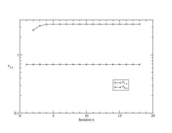
Figure 1: $e_{\lambda\,n}$ vs. n for the bound state and the spurious solution

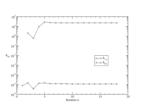
Figure 2: $\Delta_{\lambda,n}$ vs. n for the bound state and the spurious solution

Figure 1 shows the convergence for the ground state eigenvalue $e_{o\,n}$ and a spurious solution $e_{1\,n}$. After 18 iterations, $e_{o\,n}$ quickly converged to the exact ground state value of $E_{o}=\simeq 0.683729$. The unphysical spurious solution converged to a value of 3.37003. Using a larger perturbation factor of $\gamma=.95$, $e_{0\,n}$ converged to $E_{0}$ to within two significant figures after 18 iterations.

Figure 2 shows the convergence of $\Delta_{\lambda,n}$ for the ground state solution and the spurious solution. $\Delta_{\lambda,n}$ iteratively converges to zero for the generated bound state solution and converges to a non-zero value for the spurious solution.

VI Conclusions

The eigensolutions of the Dirac Hamiltonian have successfully been obtained using the the Lanczos algorithm. An eigensolution can be identified by testing the convergence of $\Delta_{\lambda,n}$ for each generated eigenpair and by discarding generated solutions for which $\Delta$ does not converge to zero. The convergence rate, needless to say , depends on the choice of the initial start vector.

Furthermore, it has been pointed out Parlett (1980) that the Lanczos algorithm may be regarded as an application of the Rayleigh-Ritz method in which an orthonormalized set of Krylov vectors have been used to define the successive subspaces in which the operator is diagonalized. This being the case, the convergence of $\Delta$ should also be a suitable means of sorting out the approximate exact eigenstates from the spurious eigenstates if the Rayleigh-Ritz method is employed.

References

- Bethe (1964) H. A. Bethe, Intermediate Quantum Mechanics (W. A. Benjamin, Inc., 1964).
- J. P. Desclaux (1975) J. P. Desclaux, Phys. Commun. 9, 31 (1975).
- I. P. Grant et al. (1976) I. P. Grant, D. F. Mayens, and N. C. Pyper, J. Phys. B 9, 2777 (1976).
- C. Krauthauser and R. Hill (2002) C. Krauthauser and R. Hill, Can. J. Phys. 80, 181 (2002).
- G. W. F. Drake and S. P. Goldman (1981) G. W. F. Drake and S. P. Goldman, Phys. Rev. A 23, 2093 (1981).
- S. P. Goldman and G. W. F. Drake (1982) S. P. Goldman and G. W. F. Drake, 25, 2877 (1982).
- S. P. Goldman and G. W. F. Drake (1988) S. P. Goldman and G. W. F. Drake, 25, 393 (1988).
- W. Kutzelnigg (1984) W. Kutzelnigg, Int. J. Q. Chem. 25, 107 (1984).
- S. P. Goldman (1985) S. P. Goldman, Phys. Rev. A 31, 3541 (1985).
- E. Ackad and M. Horbatsch (2005) E. Ackad and M. Horbatsch, J. Phys. A 38, 3157 (2005).
- J. P. Boyd et al. (2003) J. P. Boyd, C. Rangan, and P. H. Bucksbaum, J. Comput. Phys. 188, 56 (2003).
- B. Thaller (1992) B. Thaller, The Dirac Equation (Spinger, New York, 1992).
- Lanczos (1950) C. Lanczos, J. Res. Nat. Bur. Stand. 45, 255 (1950).
- Kreuzer et al. (1981) K. G. Kreuzer, H. G. Miller, and W. A. Berger, Phys. Lett. A 81, 429 (1981).
- Andrew and Miller (2003) R. C. Andrew and H. G. Miller, Phys. Lett. A 318, 487 (2003).
- Wolfram (1991) S. Wolfram, Mathematica A System for Doing Mathematics by Computer - second edition (Addison-Wesley, Redwood, California, 1991).
- Parlett (1980) B. N. Parlett, The Symmetric Eigenvalue Problem (Prentice Hall, Englewood Cliffs, N. J., 1980).
- J. J. Sakurai (1984) J. J. Sakurai, Advanced Quantum Mechanics (New York:Addison-Wesley, 1984).