A Case Study of Low-Mass Star Formation

Abstract

This article synthesizes observational data from an extensive program aimed toward a comprehensive understanding of star formation in a low-mass star-forming molecular cloud. New observations and published data spanning from the centimeter wave band to the near infrared reveal the high and low density molecular gas, dust, and pre-main sequence stars in L1551.

The total cloud mass of $\sim 160$ $M_{\odot}$ contained within a 0.9 pc has a dynamical timescale, $t_{\rm dyn}=1.1$ Myr. Thirty-five pre-main sequence stars with masses from $\sim 0.1$ to 1.5 $M_{\odot}$ are selected to be members of the L1551 association constituting a total of $22\pm 5$ $M_{\odot}$ of stellar mass. The observed star formation efficiency, ${\rm SFE}=12$%, while the total efficiency, ${\rm SFE}_{\rm tot}$, is estimated to fall between 9 and 15%.

L1551 appears to have been forming stars for several $t_{\rm dyn}$ with the rate of star formation increasing with time. Star formation has likely progressed from east to west, and there is clear evidence that another star or stellar system will form in the high column density region to the northwest of L1551 IRS5.

High-resolution, wide-field maps of L1551 in CO isotopologue emission display the structure of the molecular cloud at 1600 AU physical resolution. The ¹³CO emission clearly reveals the disruption of the ambient cloud by outflows in the line core and traces the interface between regions of outflow and quiescent gas in the line wings. Kinetic energy from outflows is being deposited back into the cloud on a physical scale $\lambda_{\rm peak}\approx 0.05$ pc at a rate, $\dot{E}_{\rm input}\approx 0.05$ $L_{\odot}$. The remaining energy afforded by the full mechanical luminosity of outflow in L1551 destroys the cloud or is otherwise lost to the greater interstellar medium.

The C¹⁸O emission is optically thin and traces well the turbulent velocity structure of the cloud. The total turbulent energy is close to what is expected from virial equilibrium. The turbulent velocities exist primarily on small scales in the cloud and the energy spectrum of turbulent fluctuations, $E(k)\propto k^{-\beta}$, is derived by various methods to have $\beta\approx 1$–2. The turbulent dissipation rate estimated using the results of current numerical simulations is $\dot{E}_{\rm diss}\approx\dot{E}_{\rm input}$.

This study reveals that stellar feedback is a significant factor in the evolution of the L1551 cloud.

1. Introduction

Low-mass stars form from dense, quiescent cores embedded within turbulent molecular clouds (Myers et al. 1983; Beichman et al. 1986; Larson 1981). Following a rapid inside-out gravitational collapse phase (Shu 1977), embedded sources accrete material from their surroundings through a disk while bipolar flows interact with the progenitor cloud (Hartigan et al. 1995; Richer et al. 2000; Reipurth & Bally 2001). Young stars become optically visible and accretion diminishes over time, as does the mass of the circumstellar disk (Hartmann et al. 1998; Lada 1991). The luminosities of the pre-main sequence stars evolve as they contract and eventually settle onto the main sequence (Hayashi 1961). This succession in the formation of low-mass stars is fairly certain, but the theoretical context in which these stages fit is still debated.

As first pointed out by Zuckerman & Evans (1974), the molecular mass in the Galaxy, $\sim 2\times 10^{9}$$M_{\odot}$ (Bloemen et al. 1986), compared to the star formation rate, $\sim 4$ $M_{\odot}$ yr^-1 (Prantzos & Aubert 1995), indicates that star formation is a globally inefficient process (see also Krumholz & Tan 2007). Another universal property of star formation is the distribution of stellar masses produced by a star-forming cloud, or the initial mass function (IMF; Meyer et al. 2000). Any successful theory of star formation will explain these general properties of star formation in a way consistent with the above scenario.

In the standard paradigm for low-mass star formation (Shu et al. 1987), magnetically sub-critical cores evolve into protostars over timescales of $\sim 10$ Myr (Ciolek & Mouschovias 1994). Upon the formation of a protostar, outflows limit the amount of material available for accretion and disperse the parent cloud. Thus feedback from young sources play a critical role in determining the final stellar masses and overall star formation efficiency. The copious energies of molecular outflows (Bachiller 1996), the large spatial extent of Herbig-Haro flows (Reipurth & Bally 2001), and the existence of remnant cavities in star-forming clouds (Quillen et al. 2005; Cunningham et al. 2006) all lend credence to this picture. However, magnetic field observations do not show strong evidence for magnetically sub-critical cores (Crutcher 1999).

In another description of low-mass star formation, ordered magnetic fields and stellar feedback are not critical elements of the process. Rather star formation occurs on the order of a dynamical timescale in regions of converging turbulent velocity fields (Ballesteros-Paredes et al. 2007; Elmegreen 2000). The inefficiency of star formation and the IMF arise solely from the properties of interstellar turbulence in this framework (Vázquez-Semadeni et al. 2005; Padoan et al. 2001; Padoan & Nordlund 2002). Turbulence in star forming regions is difficult to characterize from observational data alone (Elmegreen & Scalo 2004) and support for this theory relies heavily upon computer simulation.

The aim of this work is to gain insight into the relative importance of different mechanisms involved in the star formation process by doing a detailed case study of a star-forming region. The Lynds dark cloud L1551 (Lynds 1962) is an ideal subject for this kind of study since it is a relatively isolated, nearby ($\sim 160$ pc), star-forming cloud with a wealth of activity that encompasses all phenomena known to be associated with low-mass star formation including; a population of pre-main sequence stars (Kenyon & Hartmann 1995), multiple outflows (Snell 1981; Moriarty-Schieven & Snell 1988; Moriarty-Schieven et al. 1995; Pound & Bally 1991), jets (Mundt et al. 1990), winds (Welch et al. 2000; Giovanardi et al. 2000), an abundance of shocked gas (Devine et al. 1999), and reflection nebulosity (Draper et al. 1985). This article is based on the work by Swift (2006), and summarizes some of the conclusions therein while elaborating on some of the themes via new data and analyses.

Our new observations are presented in § 2 and contribute significantly to the numerous observations in this region. Data pertaining to the young stars around L1551 give insights into the star formation history and the cloud lifetime, and Spitzer IRAC observations of the dense core L1551-MC add to the understanding of the highest column regions of L1551 in § 3. The general properties of the L1551 cloud are then deduced in § 4 using dust extinction and ¹³CO emission.

The high-resolution CO isotopologue maps are shown in § 5 where the ¹³CO emission proves to be a good tracer of stellar feedback in L1551. The nature of this feedback is explored in § 6 where it is found that outflow in L1551 is both stirring the ambient gas as well as excavating mass from the cloud. The C¹⁸O emission traces the mass distribution in L1551 better than the ¹³CO, and these data are used to probe the turbulent velocity field in the cloud in § 7. The star formation history in L1551 is discussed in § 8, and the main conclusions of the article are summarized in § 9.

2. Observations and Reductions

2.1. Wide-Field BIMA Mosaic

A 250 pointing interferometric mosaic conducted with the BIMA interferometer covers $\sim 140$ square arcminutes of the L1551 cloud. The mosaic is designed to image the regions of highest ¹³CO emission as seen in the single-dish maps of Swift et al. (2005) including the region of L1551-MC. The full mosaic is broken into 13 sub-mosaics, labeled A–M, each consisting of roughly 20 pointings. Each sub-mosaic track was run for a full night in both the C and D array configurations while follow-up scheduling was directed to create nearly constant sensitivity across the map. Table 5.1 in Swift (2006) summarizes the observations which span 7 years with the vast majority of tracks run between 2001 and 2004. Figure 1(a) displays the pointing centers for the sub-mosaics superposed on velocity integrated ¹³CO from Swift et al. (2005).

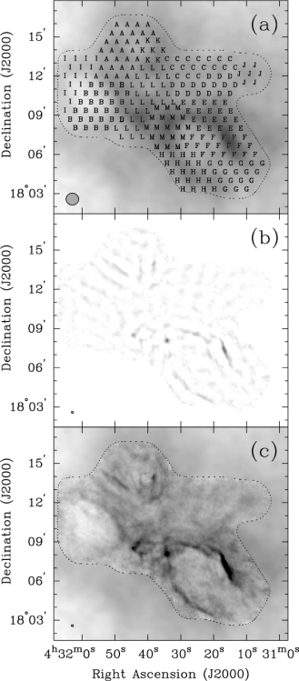
Figure 1.— (a) Velocity integrated ¹³CO$(1-0)$ emission from the Kitt Peak 12 m showing the pointings from each sub-mosaic A–M. (b) The integrated emission from the interferometer data, and (c) the combined map as described in § 2.2. The gray scale is transferred linearly between 0 and 15 K km s^-1 for all images.

The pointing coordinates in each sub-mosaic are defined in terms of right ascension and declination offsets from the most central pointing in the sub-mosaic. The offsets are chosen such that the pointing centers make a grid of equilateral triangles with each side equal to the Nyquist sampling angle, $\Theta_{\rm N}=46$″. The exception is Mosaic M where both the right ascension and declination offsets are integer multiples of $\Theta_{\rm N}$.

The mosaic data were taken in correlator mode 6 (Welch et al. 1996) with the two high-resolution windows containing 256 channels set to 12.5 MHz widths centered on the transition frequencies of C¹⁸O (109.78216 GHz) and ¹³CO (110.20135 GHz) in the upper side band. This translates to a velocity resolution of 0.13 km s^-1 in these spectral windows.

Each sub-mosaic track cycled through all pointings with 23 s integrations performed in groups of 1, 2 or 3 at each pointing center depending on mosaic size in consideration of proper phase calibration. Integrations at all pointings were performed between phase calibration for tracks with 20 pointings or less. For the larger mosaics (A, B, and L), two calibration integrations were embedded in the mosaic to ensure phase tracking. In our final data, the $u$–$v$ sampling is complete over the entire map from $2\lesssim\sqrt{u^{2}+v^{2}}\lesssim 25$ k$\lambda$. The observations were phase calibrated using nearby quasars 0530+135 and 0429+113, both $\gtrsim 1$ Jy sources at these observing frequencies throughout the program.

The flux scale was calibrated using W3(OH) as the primary calibrator. Saturn or Uranus was used as a secondary calibrator, and Jupiter was used occasionally for D configuration observations. The flux scale in the final maps is estimated to be accurate at the $\sim 15$% level.

Anomalous amplitudes and phases were flagged from the data, and no shadowed data were used. Line-length and gain calibrations were applied, and then all data were Fourier transformed simultaneously using MIRIAD (Sault et al. 1995). Natural weighting was used to maximize signal to noise. Figure 1(b) shows the positive values of the velocity integrated emission from the Fourier transform—the “dirty” map.

The maps were then deconvolved with a Steer-Dewdney-Ito CLEAN algorithm (Steer et al. 1984) using a low loop gain of 0.05 and a maximal number of iterations so that all flux above the 1 $\sigma$ level was transferred to CLEAN components. The clean image was then restored with a bivariate Gaussian clean beam having FWHM dimensions of $10.\!\arcsec 3\times 8.\!\arcsec 7$ and position angle of $29^{\circ}$.

2.2. Combining Single-Dish and Interferometer Data

A single pointing of an interferometer cannot measure visibilities where $\sqrt{u^{2}+v^{2}}<D$. Observations using multiple pointings allow the $u$–$v$ plane to be sampled slightly inside this limit due to the Ekers & Rots (1979) effect, but intensity variations on scales larger than the primary beam cannot be recovered with interferometry alone [compare Figure 1(a) and (b)]. Therefore, when mapping extended objects with interferometry the addition of single dish data is essential in reconstructing accurate depictions of the sky brightness distribution (see Holdaway 1999).

Approximately 6% of the total ¹³CO flux is recovered with our cleaned BIMA mosaic. The flux recovery is greatest in the line wings, reaching as high as $\sim 35$%, and steadily decreasing to effectively zero in the line core. The flux recovery in the C¹⁸O map is on the level of a few percent.

The flux density scales of the single-dish and interferometric datasets were compared in the region of $u$–$v$ overlap in the manner described by Stanimirović et al. (1999). The flux density scale for the Kitt Peak 12 m was consistent with the nominal scale of 33 Jy K^-1 (Helfer et al. 2003), and a flux scaling factor of unity is assumed for all data in the combination.

The data are combined using a linear combination of the two datasets followed by a maximum entropy deconvolution (Stanimirović et al. 1999; Holdaway 1999). The regridded single-dish map, seen in velocity integrated ¹³CO intensity in Figure 1(a), is first combined with the dirty BIMA mosaic using Equation 4 in Stanimirović et al. (1999). The ratio of beam areas, $\alpha=0.029$.

The maximum entropy deconvolution was performed using MIRIAD. An rms factor of 1.2 was used to account for the discrepancy between the theoretical and the real rms in the images. The regridded single-dish image served as the default image, and the total flux of the output was forced to agree with the total flux in the default image. Without using the single-dish image as the default the total flux in the final image was overestimated by nearly a factor of 2.

Convergence was achieved in all 64 image planes in $\lesssim 15$ iterations. There are no significant artifacts from the deconvolution and the overall image quality is very good. The deconvolution residuals contain minimal structure with a consistent rms from channel to channel, evidence of a successful deconvolution. The regridded single-dish map, the interferometer map, and the deconvolved combined map integrated over the ¹³CO line profile can be seen in Figure 1.

2.3. Deep Near Infrared Imaging and A Large Scale Extinction Map

Deep near infrared (NIR) imaging was obtained on the night of 2004 November 11 to supplement data from the 2MASS point source catalog (Skrutskie et al. 2006) in the L1551 region. The images were obtained with FLAMINGOS on the Kitt Peak 2.1 m telescope. FLAMINGOS is a combination wide-field, near infrared imager and multi-object spectrometer built by the University of Florida (Elston et al. 2003). In imaging mode, the $2048\times 2048$ science grade Hawaii-II HgCdTe array has a plate scale of 0.​″606 pixel^-1 and a 20.​′7 field of view.

Three sets of exposures were taken through the $J$, $H$, and $K$-band filters with total exposure times of 720, 720, and 875 s consisting of 15 45 s exposures in $J$ and $H$, and 25 35 s exposures in $K$. These data were reduced using the LONGLEGS (Román-Zúñiga et al. 2006) reduction procedure.

$J$, $H$, and $K_{\rm s}$ band photometric data from the 2MASS point source catalog were selected within a $4^{\circ}$ radius of L1551 using VizieR (Ochsenbein et al. 2000). Aperture photometry of 171 FLAMINGOS point sources matched with the 2MASS catalog produced zero points for the FLAMINGOS data to an accuracy of $\sim 0.\!\!^{\rm m}25$. The limiting magnitudes of our FLAMINGOS data are 22.3 in $J$, 21.9 in $H$, and 21.4 in $K_{\rm s}$.

The NICER method (Lombardi & Alves 2001) is an optimized technique for converting NIR color excess of background stars into an $A_{V}$ map. Using conversion factors from the literature (Harvey et al. 2003; Rieke & Lebofsky 1985), extinction values were assigned to gridded $1.\!^{\prime}2$ pixels based on a weighted mean of measured extinctions from stars falling within a $2.\!^{\prime}9$ FWHM Gaussian beam centered on the pixel coordinates. The weighting incorporates errors in photometry, errors due to intrinsic variations of stellar colors determined from a control field located at $4^{\rm h}20^{\rm m}00^{\rm s},17^{\circ}00^{\prime}00^{\prime\prime}\,(J2000)$, and the stellar position relative to the pixel center.

Figure 2 shows the extinction map of L1551 with a dynamic range of $0^{\rm m}\!\!.5\lesssim A_{V}\lesssim 18^{\rm m}$ and a mean $\langle A_{V}\rangle\approx 6$ taken over the central $20^{\prime}\times 20^{\prime}$ of the cloud. The rms in the map varies from $0^{\rm m}\!\!.6$ in the part of the map with only 2MASS data, to $0^{\rm m}\!\!.3$ in the outskirts of the Kitt Peak 2.1 m data, to more than $1^{\rm m}$ in the inner regions where there are a paucity of background stars. The errors are skewed toward higher extinction values in regions of high obscuration.

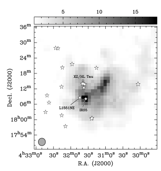
Figure 2.— Map of the measured dust extinction from the L1551 cloud in units of $A_{V}$. Known pre-main sequence stars are overlaid for reference, and the $2^{\prime}\!.9$ Gaussian smoothing kernel is shown at the bottom left.

2.4. Spitzer IRAC Imaging

A single Infrared Array Camera (IRAC; Fazio et al. 2004) footprint centered on the position of peak NH₃ emission from L1551-MC, $4^{\rm h}31^{\rm m}09^{\rm s}\!.9$, $+18^{\circ}12^{\prime}41^{\prime\prime}\,\,(J2000)$ (Swift et al. 2005), was imaged with the Spitzer Space Telescope on 23 March 2006. In 8 min of total on source integration time, a $3\,\sigma$ point source sensitivity of roughly 2, 4, 10, and 10 $\mu$Jy was achieved in the 3.6, 4.5, 5.8 and 8.0 $\mu$m bands, respectively. The post-BCD data were inspected and found to be free from artifacts in the first three bands. Small, but noticeable ($\sim 1\,\sigma$ peak) decrements in the floor value of several north-south columns produce the “jail bar effect” in our 8 $\mu$m image. Aperture photometry provided point source flux measurements (DN s^-1) using an aperture radius of 4 pixels, or $4^{\prime\prime}\!\!.8$. Zeropoint values of 280.9, 179.9, 115.0, and 64.13 Jy in the 4 respective IRAC bands convert these fluxes into magnitudes.

3. The Stellar Component

Figure 3 shows the velocity integrated CO$(1-0)$ emission from the southern end of the Taurus molecular complex (Dame et al. 2001). To the north, the majority of young stars in Taurus are being born along high density filaments (Onishi et al. 1998; Hartmann 2002). L1551 lies further out of the Galactic plane at $l\approx 179^{\circ}$, and appears as an isolated molecular clump at a distance of $160\pm 20$ pc (Bertout et al. 1999; Snell 1981).

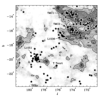
Figure 3.— Southern part of the Taurus molecular complex in CO$(1-0)$ emission shown in gray scale (0–25 K km s^-1) and contours (6, 12 and 18 K km s^-1) (Dame et al. 2001) with the positions of pre-main sequence stars (star symbols) overlaid (Palla & Stahler 2002, also see Table A Case Study of Low-Mass Star Formation). L1551 is seen as a relatively isolated molecular clump coincident with an association of young stars. The positions of well-known star-forming clouds TMC 1, TMC 2, and L1536 as well as T Tau are labeled.

There is an association of pre-main sequence (PMS) stars centered near the peak CO column density of L1551. Table A Case Study of Low-Mass Star Formation displays 70 PMS stars within a $4^{\circ}$ radius of L1551. There have been numerous searches for PMS stars in this region (Herbig & Bell 1995; Feigelson et al. 1987; Gomez et al. 1992; Briceño et al. 1998, 2002; Luhman 2000) and it is expected that all PMS stars within the central square degree have been identified. Many searches for companion stars have also been conducted in this region sensitive to separations between 1 and 2000 AU (Kohler & Leinert 1998; Simon et al. 1995; Ghez et al. 1993; Leinert et al. 1993; Reipurth & Zinnecker 1993), and a large fraction of companion stars are presumed to be known.

3.1. Selection

Stars with a high probability of having formed from the L1551 cloud are chosen from the list in Table A Case Study of Low-Mass Star Formation according to their proper motions and radial velocities where possible, as well as the projected spatial distribution.

The 34 proper motion entries listed in Table A Case Study of Low-Mass Star Formation have typical measurement errors of 0.5 arcseconds per century (Ducourant et al. 2005) translating to a $\sim 5$ km s^-1 error on the two-dimensional space motions. The mean proper motion for this sample is $\langle\Delta\alpha,\Delta\delta\rangle=(0.71\pm 0.1,-1.5\pm 0.1)$ arcseconds per century. There are three outliers in the distribution of proper motions that lie beyond 15 km s^-1 of the mean—RX J0433.7+1823, RX J0430.8+2113, and RX J0444.4+1952—and are rejected from the sample.

The distribution of 21 radial velocities have a mean of 5 km s^-1 (LSR) and a dispersion consistent with the quoted measurement errors for this sample, $\sim 2$ km s^-1 (Herbig & Bell 1995). The only clear outlier in this distribution is DQ Tau, and it is rejected based on this criterion.

Figure 4 shows the projected radial distribution of all PMS stars from Table A Case Study of Low-Mass Star Formation. The stellar density drops smoothly to zero and then persists at a roughly constant, low level beyond $2^{\circ}$. Based on this distribution, all stars beyond a $1.\!\!^{\circ}6$ radius from L1551 are rejected from our sample.

Figure 4.— Histogram of the number of pre-main sequence (PMS) stars within $0.\!\!^{\circ}25$ bins of projected radius from L1551. There is an absence of PMS stars between $1.\!\!^{\circ}6$–$2.\!\!^{\circ}1$, and this gap is used to separate the L1551 candidates (cross-hatched area) from PMS stars in the field that are less likely to have formed in L1551.

Of the spatially selected PMS population, 5 have unknown spectral types and 1 has inadequate photometry. These stars are flagged from the sample. Main-sequence colors (Kenyon & Hartmann 1995) are assumed for weak-line T-Tauri stars (wTTSs) and the NIR color-color locus from (Meyer et al. 1997) is assumed for classical T-Tauri stars (cTTSs). Seven stars in the sample have NIR colors that are suspect or inconsistent with these assumptions and they are marked with a “C” in Table A Case Study of Low-Mass Star Formation. Six of these seven have adequate supplementary data from the literature that are used in further analyses, while the remaining source, RX J0437.4+1851 A, is flagged. The number of stars used in the following analyses totals 37 (39 if the binary companions to L1551 IRS5 and L1551 NE are counted), 7 (9) of which are embedded. There are 29 stellar systems and 10 companions in the sample for a companion star fraction of 34%. This is lower than, but comparable to the measured companion star fraction in large samples of young stars (e.g., Kohler & Leinert 1998).

3.2. The Hertzsprung-Russell Diagram

The spectral types of the PMS stars are converted to effective temperatures using Kenyon & Hartmann (1995, Table A5) for spectral types earlier than M0 and Luhman et al. (2003, Table 8) for later spectral types. Effective temperatures for fractional spectral types are computed by interpolation.

Figure 5.— Hertzsprung-Russell diagram for the 30 stars that passed our selection criteria of § 3.1 (embedded sources are excluded). The assumed error in luminosity is shown at the bottom left (see § 3.2). Pre-main sequence evolutionary tracks for masses between 0.1–1.2 $M_{\odot}$ and ages between 1–20 Myr are overlaid (Baraffe et al. 1998, 2002). The two stars to the upper left, TAP 51 and HBC 407, lie near the main sequence (dashed line) and are likely interlopers.

The extinction toward each source is derived by tracing the reddening line back to either the cTTS locus or the main sequence, otherwise literature values are used. The NIR fluxes were then corrected according to the models of Rieke & Lebofsky (1985). Bolometric luminosities are computed by applying a bolometric correction to the extinction corrected $J$ band magnitude, $J_{\rm c}$. Kenyon & Hartmann (1995, Table A5) is used for spectral types earlier than M0, Bessell (1991, Table 2) for spectral types M0 through M7 and Reid et al. (2001, Table 2) for spectral types M8 through M9.5.

Figure 5 displays the selected sample of PMS stars, excluding embedded sources, on the theoretical Hertzsprung-Russell diagram. A subset of the PMS evolutionary tracks by Baraffe et al. (1998, 2002) are overlaid. The errors on the data points in this plot are based on arguments by Hartmann (2001). Our assumed error of $\delta\log L=0.16$ is somewhat conservative since this suggested value was derived assuming all stars to have unresolved companions while it is expected that most, if not all, companion stars in our final sample are resolved. No error is assumed on the effective temperatures since, in conjunction with the bolometric correction, these errors will have a small effect on the derived ages.

3.2.1 Derived Stellar Properties

Table A Case Study of Low-Mass Star Formation displays the ages and masses of the L1551 population derived from the evolutionary models of Baraffe et al. (1998, 2002) along with the type, class (Lada 1987; Adams et al. 1987), and the derived $A_{V}$ and $J_{\rm c}$ values. The errors in the determined age are calculated by re-deriving these quantities for $\log L\pm\delta\log L$. The errors in mass are estimated to be $\lesssim 25$% for a half spectral type uncertainty. Two stars fall very near the zero-age main sequence—HBC 407, and TAP 51—and are heretofore rejected based on the likelihood that they are interloping main-sequence stars.

Figure 6 shows the cumulative age distribution of pre-main sequence stars in L1551. Each bin value represents the number of stars associated with L1551 that have ages greater than or equal to the age value of the bin, and the errors are determined using a Monte-Carlo technique. There are a total of 35 stars in this sample, 28 have theoretical ages from Figure 5, and the 7 embedded sources assumed to have ages $<1$ Myr fall within the first bin. The total stellar mass of this sample is $22\pm 5$ $M_{\odot}$.

The majority of the selected PMS stars have ages less than 4 Myr. However, both age distributions in Figure 6 derived from independent PMS evolutionary models show that $\sim 20$% of the stars in this region formed more than 6 Myr ago. While the derived age spread in this region is larger than the age spread typically stated for the Taurus complex as a whole (e.g., Ballesteros-Paredes et al. 1999; Hartmann et al. 2001), these results are consistent with previous studies (Gomez et al. 1992; Palla & Stahler 2002).

Figure 6.— Cumulative histogram of pre-main sequence ages for the L1551 association derived from the Hertzsprung-Russell diagram. Each 2 Myr bin represents the number of stars with ages greater than or equal to the bin age. The solid line represents the ages obtained with models of Baraffe et al. (1998, 2002) and the dotted line represents the ages obtained with the Palla & Stahler (1999) models.

3.3. The Spatial Distribution of the PMS Population

The radial distribution of PMS stars in L1551 is concentrated near the center of the cloud, and decreases to zero at a radius of $R_{\rm stars}=1.\!\!^{\circ}6$, or 4.5 pc in projected distance. The dispersion timescale for the stellar association is estimated

$$t_{\rm disp}^{*}=\frac{\pi}{2}\frac{R_{\rm stars}}{\sigma_{\rm 3D}^{*}}$$ (1)

where $\sigma_{\rm 3D}^{*}$ is the three-dimensional velocity dispersion of the stars, and the factor of $\pi/2$ accounts for a random inclination angle of stellar motion with respect to the line of sight. The dispersions of the proper motion and radial velocity distributions of the L1551 association are approximately equal to the stated measurement errors (Ducourant et al. 2005; Herbig & Bell 1995). Therefore an upper limit on the one-dimensional velocity dispersion for the stellar association of 2 km s^-1 results from the dispersion of radial velocities. A lower limit of 0.3 km s^-1 is derived from the velocity dispersion of C¹⁸O emission in the cloud (§ 7).

For a one-dimensional velocity dispersion of 1 km s^-1 ($\sigma_{\rm 3D}=\sqrt{3}\sigma_{\rm 1D}$), $t_{\rm disp}^{*}\approx 4$ Myr. The observed spatial distribution of stars is thus consistent with dispersion by random motions over several million years. It is also possible that the stars formed in their observed locations within the last $\sim 1$ Myr, but this seems less likely given the distribution of molecular gas in relation to the stellar positions and the high fraction ($\sim 50$%) of wTTSs in the association.

The radial distribution of stars fans out to the east, and there are significantly more stars to the east of the cloud center than the west (see Figures 2 and 3). Moriarty-Schieven et al. (2006) argue that L1551 is being eroded from the east by ionizing flux, perhaps from Orion, and the PMS stellar distribution is modest support for their conclusion that star formation is progressing predominantly from east to west.

Although we are only observing projected separations, the spatial distribution of embedded stars does not appear to follow any particular prescription such as Jeans fragmentation. All embedded stars appear in regions of stellar activity suggesting that triggering may be an important process (e.g., Yokogawa et al. 2003). However, the fact that the next star or stellar system in L1551 appears to be forming from quiescent gas (§ 3.4) counters this notion.

3.4. Future Star Formation

A gravitationally bound, 2–3 $M_{\odot}$ pre-protostellar core was recently discovered in a quiescent region to the northwest of L1551 IRS5 (Swift et al. 2005; Moriarty-Schieven et al. 2006). Follow up observations of this core, named L1551-MC, confirm the existence of high volume density gas and reveal $\gtrsim 0.1$ km s^-1 infall signatures (Swift et al. 2006). The gas motions related to the redshifted self-absorption in the CS line profiles are associated with build up of core mass, and it is probable that a star or stellar system will form in this region in $\lesssim 1$ Myr. However, the existence of a very low luminosity object (Kauffmann et al. 2005) embedded in L1551-MC has not yet been ruled out.

Figure 7 shows a composite image of L1551-MC made from all four IRAC bands. There is a deficit of emission along the central dust lane in the 8 $\mu$m band due to the extinction of the Galactic background at these wavelengths. In the 3.6 and 4.5 $\mu$m bands there is excess emission along the lane due to scattered light. There is no evidence for an embedded source within an arcminute of the peak NH₃ emission in our IRAC data. An upper limit of $L_{\rm bol}<0.005$ $L_{\odot}$ is set from the sensitivity of our 8 $\mu$m IRAC image using a bolometric temperature of 100 K.

Figure 7.— Spitzer IRAC composite image of L1551-MC with blue $=3.6\,\mu$m, green $=4.5\,\mu{\rm m}+5.8\,\mu{\rm m}$, and red $=8.0\,\mu$m. The position of peak NH₃ emission from Swift et al. (2005) (white cross) and an ellipse enclosing the highest column density region of the map are shown.

Two 24 $\mu$m sources appear near L1551-MC in MIPS archival data (Campaign ID: 713). The brighter source has a flux $\sim 1$ Jy and is located at $4^{\rm h}31^{\rm m}05^{\rm s}\!\!.7$,$+18^{\circ}13^{\prime}21^{\prime\prime}\,\,(J2000)$. This source has no counterpart in any of the IRAC bands and shows a systematic $0^{\prime\prime}\!\!.22$ s^-1 motion relative to another point source in the MIPS field. It is likely this source is an asteroid. The weaker source is located at $4^{\rm h}31^{\rm m}07^{\rm s}$,$+18^{\circ}13^{\prime}17^{\prime\prime}\,\,(J2000)$ and is coincident with an extended source apparent in all IRAC bands. This object may be either multiple sources along the line of sight or a background galaxy.

The 3.6 and 4.5 $\mu$m images are used to estimate the total visual extinction inside and outside the central $\sim 2^{\prime}\times 3^{\prime}\!.5$ region of L1551-MC shown in Figure 7. The mean $[3.6]-[4.5]$ color of stars inside this oval translates to $\langle A_{V,in}\rangle=42^{\rm m}\pm 4^{\rm m}$. The colors of background stars outside the oval give $\langle A_{V,out}\rangle=19^{\rm m}\pm 3^{\rm m}$, consistent with the NIR measurements in this region.

A low-mass star or stellar system is likely to form within the high column dust lane extending northwest from L1551 IRS5, and these new Spitzer data show that a low luminosity protostar has yet to form in the L1551-MC region. Given the limited extent of the dust lane (see Figure 2), it is unlikely that a significant number of stars will form in the future. However, further study is needed to determine the gravitational stability of the gas northwest of L1551-MC.

4. General Properties of the L1551 Cloud

4.1. Mass and Abundances

The visual extinction shown in Figure 2 is converted to total hydrogen column using Bohlin et al. (1978) and an extinction curve slope, $R_{V}=3.1$, giving $N$(H${}_{\rm tot})=1.9\times 10^{21}\,A_{V}$ cm^-2. Summing over the entire cloud yields a mass of $M_{\rm H}\approx 120$ $M_{\odot}$. Correcting for a helium abundance, $Y_{\rm p}=0.25$, the total mass of L1551 $M_{\rm tot}\approx 160$ $M_{\odot}$. This value is higher than all previous estimates of the ambient cloud mass made using CO isotopologue emission (e.g., Snell et al. 1980; Stojimirović et al. 2006). CO fails to trace areas of low extinction due to photodissociation and also suffers saturation effects in high column regions. These effects are expected to account for the discrepancies.

Assuming local thermodynamic equilibrium (LTE) conditions, the optical depth of both ¹³CO$(1-0)$ and C¹⁸O$(1-0)$ can be estimated over the central $20^{\prime}\times 20^{\prime}$ of L1551 (Swift et al. 2005, Equation 3). The maximum ¹³CO optical depth in L1551 is computed to be $\tau_{\rm 13,max}\sim 10$, and the mean $\langle\tau_{13}\rangle\sim 2$. The C¹⁸O emission is optically thin everywhere.

A pixel by pixel comparison of our $A_{V}$ map with the regridded CO isotopologue maps gives a conversion between magnitudes of visual extinction and total CO isotopologue column. We assume a constant excitation temperature of 15 K for the molecular gas, although variations from 9 to 25 K may exist (Swift et al. 2005; Stojimirović et al. 2006; Snell 1981). There is a linear correlation between both the $\tau$-corrected ¹³CO and the C¹⁸O column depth with $A_{V}$ between $\sim 2$ and $10^{\rm m}$. For $A_{V}\gtrsim 10^{\rm m}$ the scatter in the relation becomes large and the CO derived column depths appear to saturate. Linear fits to the column depths as a function of $A_{V}$ between 0 and $10^{\rm m}$ give

$$N(^{13}{\rm CO})=(2.5\pm 0.1)\times 10^{15}\,(A_{V}-0.8\pm 0.3)\,{\rm cm}^{-2}$$ (2)

$$N({\rm C}^{18}{\rm O})=(2.6\pm 0.2)\times 10^{14}\,(A_{V}-2.2\pm 0.4)\,{\rm cm}^{-2}$$ (3)

with the 1 $\sigma$ error estimates from the fits included explicitly.

These numbers agree well with past studies (e.g., Dickman 1978; Lada et al. 1994). Using Bohlin et al. (1978), the abundance of ¹³CO is $1.3\pm 0.05\times 10^{-6}$ for $A_{V}$ between 0.8 and $10^{\rm m}$, and the abundance of C¹⁸O is $1.4\pm 0.07\times 10^{-7}$ relative to the total hydrogen content. Using an excitation temperature of 25 K increases the abundance of the isotopologues by $\sim 25$%.

4.2. Energy

The gravitational energy of L1551 depends on the total mass and the distribution of matter. A radial profile is computed using averages of the $\tau$-corrected ¹³CO and $A_{V}$ maps within circular annuli centered on the C¹⁸O intensity weighted mean position of L1551, $4^{\rm h}31^{\rm m}24^{\rm s}$, $+18^{\circ}10^{\prime}00^{\prime\prime}\,\,(J2000)$. Figure 8 shows this column density profile from $\sim 0.02$ to 2 pc. The error bars for each value are determined from the rms deviation of pixel values and the number of pixels in each annulus. The errors derived for the ¹³CO data lie within the symbols. The profile is flattened in the inner region of L1551 and becomes progressively steeper out to the edge of the cloud, $R_{\rm cloud}=0.9$ pc.

Figure 8.— Normalized column density profile of the L1551 dark cloud derived from both $\tau$-corrected ¹³CO emission (open circles) and near infrared extinction (filled circles). The maximum averaged column density is $\langle N({\rm H}_{\rm tot})\rangle_{\rm max}=2.2\times 10^{22}$ cm^-2.

For a density profile

$$\rho(r)=\begin{cases}\rho_{0}&;\quad 0\leq r\leq R_{\rm core}\\ \rho_{0}\left(R_{\rm core}/r\right)^{2}&;\quad R_{\rm core}\leq r\leq R_{\rm cloud}\\ \end{cases}$$ (4)

with $R_{\rm core}=0.1$ pc, $R_{\rm cloud}=0.9$ pc, and $M_{\rm tot}=160$ $M_{\odot}$, the gravitational energy

$$E_{\rm grav}^{\rm core}=-\frac{3}{5}\frac{GM_{\rm core}^{2}}{R_{\rm core}}\left[1+5\frac{\left(R_{\rm cloud}-R_{\rm core}\right)}{R_{\rm core}}\right]$$ (5)

is $-8.7\times 10^{44}\,{\rm ergs}$,where $\rho_{0}=1.9\times 10^{-19}$ g cm^-3 is found by normalizing the total mass to 160 $M_{\odot}$, and $M_{\rm core}=4/3\,\pi\rho_{0}R_{\rm core}^{3}$. An upper limit to $E_{\rm grav}$ is given by the gravitational energy of a truncated, singular isothermal sphere (SIS) with the total mass and radius of L1551, $E_{\rm grav}^{\rm SIS}=-GM^{2}/R=-2.5\times 10^{45}$ ergs. In light of these calculations, we use a gravitational energy of $E_{\rm grav}=-1\times 10^{45}$ ergs in further analyses with a factor of $\lesssim 2$ uncertainty.

The turbulent velocity width derived from the composite C¹⁸O spectrum (see § 7) is $\sigma_{\rm turb}=0.52$ km s^-1. The one-dimensional thermal width of the molecular gas

$$\sigma_{\rm therm}=\left(kT/\bar{m}\right)^{1/2}$$ (6)

is 0.23 km s^-1 for $T=15$ K and $\bar{m}=2.3\,m_{\rm H}$. Adding in quadrature the turbulent and thermal contributions gives the three-dimensional velocity dispersion of the gas in L1551, $\sigma_{\rm v}=0.65$ km s^-1. The total kinetic energy is thus $6.8\times 10^{44}$ ergs, very near what the virial theorem predicts given our estimation of $E_{\rm grav}$.

4.3. Timescales and the Jeans Criterion

Approximating L1551 as a homogeneous sphere with density $\langle n\rangle\approx 1000$ cm^-3 and mean particle mass $\bar{m}=2.3\,m_{\rm H}$, the free-fall timescale $t_{\rm ff}=\left[3\pi/(32\,G\,\rho)\right]^{1/2}=1.1$ Myr. The dynamical timescale of the cloud is taken to be equal to the free-fall timescale, $t_{\rm dyn}=t_{\rm ff}$. The sound crossing time in L1551 is estimated as $t_{\rm cross}=2\,R_{\rm cloud}/c_{\rm s}=7.7$ Myr for $c_{\rm s}=\left(kT/\bar{m}\right)^{1/2}$ and $T_{\rm k}=15$ K. This means that L1551 cannot be supported by thermal pressure alone. A varying temperature structure could alter this number significantly. However, a kinetic temperature of $>700$ K would be needed for $t_{\rm cross}=t_{\rm ff}$.

Another assessment of the balance between thermal pressure and gravity is given by the Jeans criterion (Jeans 1961). For a uniform, isothermal gas of density $\rho$, perturbations exceeding a length scale of $\lambda_{\rm J}=\left(\pi c_{\rm s}^{2}/G\rho\right)^{1/2}$ will be unstable to gravitational collapse. This length scale in L1551 is $\lambda_{\rm J}\approx 0.8$ pc—about half the cloud diameter—meaning it is Jeans unstable. Therefore other mechanisms, such as magnetic fields or turbulence, must contribute to the overall gravitational stability of the cloud to prevent a global collapse.

Unfortunately, little is known about the magnetic field in L1551 (see § 8). However in the next few sections, a closer look at the molecular gas in L1551 gives insight into sources and dissipation of kinetic energy that are keeping this cloud close to virial balance.

5. The Molecular Gas at High-Resolution

The ubiquity of outflow from young stellar objects and the presence of $\sim 35$ proto- and pre-main sequence stars associated with L1551 imply a complex relationship between the stars and the gas in L1551 over its lifetime. The interplay between young stars and the gas from which they formed is best revealed in our fully sampled, high-resolution images of ¹³CO and C¹⁸O emission.

5.1. Velocity Integrated Emission

Figure 9.— Velocity integrated ¹³CO$(1-0)$ emission of the combined interferometric and single-dish data. The image maximum is 20.6 K km s^-1. The axes are labeled in reference to the position of L1551 IRS5, $4^{\rm h}31^{\rm m}34^{\rm s}\!\!.1$, $+18^{\circ}08^{\prime}04^{\prime\prime}\,\,(J2000)$. Sources are shown as crosses and the locations of selected HH objects are marked with triangles. The thin lines represent the jet directions from the embedded sources and the resolution of the inner and outer regions of the map are shown at the bottom left.

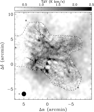
Figure 10.— Same as Figure 9 but for the velocity integrated C¹⁸O$(1-0)$ emission. The maximum pixel value in the map is 5.5 K km s^-1 at the position of L1551 IRS5, but the linear stretch has been adjusted to bring out lower level features. Note the sky coverage for the C¹⁸O data is not exactly the same as the ¹³CO data.

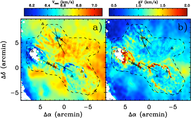
Figure 11.— The first and second “moment” maps of the ¹³CO emission in L1551 derived from Gaussian fitting. Sources and HH objects from Figure 9 are shown as well as the jet directions from the embedded sources. Spectra with ¹³CO line peaks below 3 $\sigma$ produce unreliable fits and are masked in white. The dashed black line encloses the high-resolution data.

Figures 9 and 10 show the velocity integrated ¹³CO and C¹⁸O emission from L1551, respectively. These maps have been created by summing $\sum T_{A}^{*}\Delta V_{\rm ch}$ over the line profile, where $\Delta V_{\rm ch}=0.13$ km s^-1 is the channel width. The high-resolution data are shown within the dashed contour, while outside this boundary there are only single-dish data. The C¹⁸O data cover a smaller range in right ascension but a slightly larger range in declination.

The ¹³CO map shows a smooth overall distribution of emission with clearly delineated features around regions of known stellar energetics. Two caliper-like arcs of emission to the southwest of L1551 IRS5 trace the boundary of the southwest cavity from the well known L1551 IRS5 bipolar outflow (Snell et al. 1980; Draper et al. 1985; Moriarty-Schieven et al. 1987; Moriarty-Schieven & Snell 1988; Moriarty-Schieven et al. 2006; Stojimirović et al. 2006). Northeast of L1551 NE, a sharp edge in the ¹³CO map creates a parabolic shape that is symmetric around the L1551 NE jet (Reipurth et al. 2000), though the lower arm is less pronounced than the upper. There is a deficit of ¹³CO emission within this feature that correlates with a low extinction derived from background stars (see Figure 2), and we refer to this region henceforth as the northeast cavity. The gas around XZ/HL Tau shows clear signs of disruption, likely due to jets (Mundt et al. 1990) as well as less collimated outflow seen in the region (Krist et al. 1999; Coffey et al. 2004; Welch et al. 2000).

The C¹⁸O emission is more clumpy than the ¹³CO emission and follows more closely the distribution of $A_{V}$. Most features seen in C¹⁸O correlate with features seen in ¹³CO, but there are a few notable differences. The northwest region of the ¹³CO map near HH 265 is relatively featureless, while the smooth lane of extinction that encompasses L1551-MC is noticeable in C¹⁸O. A linear feature seen in C¹⁸O extending southwest from the XZ/HL Tau region has no counterpart in the ¹³CO map, and the southern edge of the southwest outflow lobe from L1551 IRS5 is not detected in C¹⁸O.

5.2. ¹³CO Velocity Centroids and Widths

Figure 11 shows the first and second “moment” maps of the ¹³CO emission. Gaussian fitting of the ¹³CO line profile in each independent, $10^{\prime\prime}\times 10^{\prime\prime}$ pixel produced a velocity centroid, $V_{\rm cen}$ (left panel) and velocity full width at half maximum, $\Delta V=2\sqrt{2\ln 2}\sigma$ (right panel) used to construct these maps. The Gaussian shape is a decent representation of the ¹³CO line profile with $\sim 85$% of the fits having $\chi^{2}$ values less than 2.

The intensity weighted mean velocity of the ¹³CO emission is 6.7 km s^-1. Some of the smallest values of $V_{\rm cen}$ lie along the border of the southwest lobe of the L1551 IRS5 flow. The diffuse emission in the northeast cavity also has very blue central velocities likely due to outflow (see § 5.3). The red velocities at the western edge of the map are related to the L1551W flow (Pound & Bally 1991; Moriarty-Schieven & Wannier 1991; Stojimirović et al. 2006). Variations at the 0.2 km s^-1 level are found across the map that loosely correlate with features in Figure 9.

The regions where young stars are injecting energy into the cloud can be clearly identified in the velocity width map shown in Figure 11 (b). The peak line widths exceed 2 km s^-1 in a very thin ($\lesssim 1600$ AU in some sections) rim around the southwest lobe of L1551 IRS5 and in the northeast cavity. High line widths are also seen around HL/XZ Tau and in the L1551W flow region. The mean ¹³CO line width in L1551 is 0.96 km s^-1 with a variance of $\sim 0.05$ km s^-1.

The ¹³CO velocity widths in Figure 11(b) are a proxy for the kinetic energy in the gas along each line of sight. The velocity widths are only significantly above average in the regions directly associated with the energetics from young sources. Small spatial regions containing high line widths like the border of the southwest lobe have small diffusion timescales and suggest that these structures are the result of current outflow activity. Stellar feedback is the most significant source of energy input in the cloud, and the only source noticeable in our ¹³CO data.

5.3. The Spatial and Kinematic Distribution of ¹³CO

The nature and relevance of the features seen in Figures 9 and 11 are further revealed in the ¹³CO channel maps. Figure 12 shows the structure of L1551 at velocity intervals chosen to highlight the numerous features in the ¹³CO data cube. The central velocity of each map is increasingly blueward of the line center in images (a)–(d) and increasingly redward in images (e)–(h). Each channel map is depicted with a linear transfer function for the gray scale shown to the right of the plot adjusted to cover all integrated intensities from the $2.5\sigma$ level to the maximum value in each map. These values are; (a) 0.40–7.4 K km s^-1; (b) 0.33–7.6 K km s^-1; (c) 0.35–4.1 K km s^-1; (d) 0.30–3.4 K km s^-1; (e) 0.45–6.5 K km s^-1; (f) 0.45–3.2 K km s^-1; (g) 0.33–3.3 K km s^-1; (h) 0.35–2.1 K km s^-1.

Figure 12.— Channel maps of ¹³CO emission in L1551. The positions of all known embedded sources (crosses), selected HH objects (triangles), and jet directions from sources (thin lines) are shown. See the text for a detailed description of these maps.

5.3.1 Synopsis of Channel Maps

In the line core channel maps (a) and (e) much of the emission is optically thick, and the disruption of the ambient gas by outflows creates the most apparent features. In channel map (a), the northeast cavity appears as an elliptical hole with its major axis aligned with the L1551 NE jet, and the southwest cavity is outlined by a thin parabolic arc. The limb brightened shell around XZ Tau investigated in depth by Welch et al. (2000), is apparent along with a few linear structures to the east of the XZ/HL Tau region.

In channel map (b), the diffuse, blueshifted emission in the northeast cavity responsible for the small $V_{\rm cen}$ values in this region [Figure 11 (a)] is clearly visible. The bright limb around the southwest lobe becomes a dominant feature at these velocities, and the brightest emission emanates from a thin wall of compressed molecular gas just downstream from HH 102. Low level emission present near the “mouth” of the southwest cavity lies along the axis of the L1551 NE jet.

Moving further into the blueshifted line wing in channel maps (c) and (d), the bright rim of the southwest cavity persists. The emission within the main L1551 IRS5 flow moves downstream but remains compact and roughly aligned with the L1551 NE jet. Knots of emission appear around the XZ/HL Tau region.

On the red side of the ¹³CO line core shown in channel map (e), three regions of proto-stellar disruption are visible, the southwest cavity associated with the L1551 IRS5 outflow, the northeast cavity, and the XZ/HL Tau region. The southwest cavity is outlined by a complex pattern, while the northeast cavity shows a sharp upper boundary. The lower edge to the XZ Tau bubble is prominent while the emission to the north of XZ Tau appears fragmented.

In channel map (f) the emission is broken up into a network of thin filaments. The lower rim of the XZ Tau bubble is clearly visible and extends to the position of HH 30 IRS. The upper limb of the northeast cavity has a filamentary appearance at these velocities. Northeast of L1551 IRS5, between L1551 IRS5 and L1551 NE, there are a series of arcs and knots of emission. Perhaps the most interesting is the arc that intersects the position of L1551 IRS5 and may trace the boundary of its red outflow lobe. The bright emission west of HH 102 remains a prominent feature, and the L1551W flow (Pound & Bally 1991; Moriarty-Schieven & Wannier 1991) appears filamentary in the high resolution part of the map.

Continuing further into the red-shifted velocities in channel maps (g) and (f) the arc intersecting L1551 IRS5 persists but moves gradually northeast and fades with increasing velocity. A few knots of emission remain in the highest redshifted velocity map likely associated with the red lobe of the main L1551 IRS5 flow.

5.3.2 Discussion

The high-resolution ¹³CO data show a wealth of structure never before seen in this well-studied region. It is clear from this map that energy from embedded sources has accelerated ambient cloud gas. Some of this gas resides in the line wing emission. A vast majority of the features in the optically thin ¹³CO line wings appear as thin arcs of emission. A low filling factor has been deduced for the L1551 flow by Snell et al. (1984) from low-resolution data, and the structure seen in the ¹³CO line wings of Figure 12 is consistent with their value of $\sim 0.3$.

The diffusion timescale of distinct features seen in the channel maps can be estimated by dividing the size of the feature by the width in velocity space, $t_{\rm diff}\sim\Delta x/\Delta v$. Typically, $\Delta x\sim 0.05$ pc (see § 7.2) and $\Delta v\sim 1$ km s^-1, giving $t_{\rm diff}\sim 10^{5}$ years. The coherence in both position and velocity space of the filamentary structures seen in the ¹³CO line wings along with the short implied diffusion timescales leads us to interpret them as the shocked gas boundaries separating quiescent gas from outflow motions from young sources (see also Barsony et al. 1993). The velocity widths of these features do not extend much beyond the escape velocity of the cloud, $\sim 2$ km s^-1, and will likely continue to decelerate into the ambient gas. The large Reynolds numbers of these flows imply that they are highly turbulent.

6. Stellar Feedback

The high-resolution maps of § 5 show that energy is being injected into the ambient cloud from where known embedded sources exist. We look at three particular regions that show clear signs of stellar feedback—the southwest lobe of the L1551 IRS5 outflow, the northeast cavity, and the XZ/HL Tau region—to gain insight into the how stellar feedback is affecting the molecular environment of L1551.

6.1. The Expanding Shell from the L1551 IRS5 Outflow

The blueshifted, or southwest, lobe of the L1551 IRS5 outflow appears as a thin, limb-brightened shell in Figures 9, 10 and 12. The position-velocity ($p$-$v$) cuts shown in Figure 13 oriented perpendicular to the L1551 IRS5 outflow axis reveal the kinematic nature of this feature.

Figure 14 shows the emission in $p$-$v$ cuts (a)–(d) in order of increasing distance from L1551 IRS5. Along cut (a) a full arc of emission blueward of the line core can be seen. This $p$-$v$ signature is what is expected from an expanding shell with a velocity of $\sim 2$ km s^-1. Moving further away from L1551 IRS5 in cuts (b) and (c), the shell walls appear spatially thin, $\sim 0.02$ pc, and have large velocity widths. Beyond velocities 3–4 km s^-1 from the line core the shell boundaries become discontinuous in $p$-$v$ space, and in cut (d) no significant amount of emission appears at high velocity. This suggests that the expanding shell has burst out the front side of L1551, in accord with previous interpretations of observational data (e.g., Draper et al. 1985; Moriarty-Schieven & Snell 1988; White et al. 2000). The dynamical age of this feature from its diameter, $\sim 4^{\prime}\!.5$, and expansion velocity $\sim 2$ km s^-1, is roughly $10^{5}$ years

Figure 13.— Velocity integrated ¹³CO emission as in Figure 9 with the position-velocity cuts through the blue lobe of the L1551 IRS5 outflow overlaid (a–d). The positions of L1551 IRS5 and prominent HH objects (triangles) are labeled, and the direction of the L1551 IRS5 jet is shown (arrow).

Figure 14.— ¹³CO emission in the position-velocity cuts across the blue lobe of the L1551 IRS5 outflow at a position angle of $135^{\circ}$, roughly perpendicular to the L1551 IRS5 outflow axis. The projected distances of the cuts from L1551 IRS5 are $\sim 0^{\prime}\!\!.5$, $1^{\prime}$, $1^{\prime}\!\!.5$, and $2^{\prime}$ for (a), (b), (c), and (d), respectively (see Figure 13). The gray scale follows a linear transfer function from 0.3–7 K and the contour levels are 0.9, 1.5, and 2.1 K. The zero position roughly delineates the outflow axis of symmetry.

The symmetry of this expanding shell is not aligned with then known direction of the L1551 IRS5 jet (Mundt & Fried 1983) as seen in Figure 13. Yet the shell wall is spatially thin, $\sim 0.02$ pc, and has a large spread in velocity, $\sim 3$ km s^-1, implying a short dispersion timescale, $\Delta x/\Delta v\sim 10^{4}$ years. High velocity H i seen in the outflow lobes of L1551 IRS5 (Giovanardi et al. 2000) may contribute to the acceleration of this shell and its spatially thin structure.

Summing the emission in the blue lobe at LSR velocities less than 6 km s^-1 gives a total mass of $\sim 3$ $M_{\odot}$. This is taken to be a lower limit to the total shell mass since the shell also contains a component at the line-of-sight velocity of the ambient gas (see Figure 14). The energy in the expanding shell estimated by converting ¹³CO emission to mass (§ 4.1) and summing $1/2\,M|v-V_{\rm cen}|^{2}$ in each velocity channel less than 6 km s^-1 is $\sim 8\times 10^{43}$ ergs.

The total mass traced by molecular emission in the entire blue lobe of the L1551 IRS5 outflow is higher than the value derived for the shell (Stojimirović et al. 2006). However, the high velocity gas concentrated toward the center of the outflow lobe seen in CO will most likely end up in the diffuse interstellar medium rather than the L1551 cloud. The existence of HH objects beyond the edge of the cloud (see Devine et al. 1999; Moriarty-Schieven et al. 2006; Stojimirović et al. 2006) and the reflection nebulosity emanating from L1551 IRS5 (Draper et al. 1985) is further evidence that a fraction of the accelerated ambient gas is being lost from the cloud.

An estimate for the mass of excavated material can be made by calculating the decrement of ¹³CO emission inside the southwest cavity relative to the ambient cloud. Using Equation 2, the total mass excavated from the southwest lobe is of order $\sim 2$ $M_{\odot}$.

6.2. The Northeast Cavity

The lack of CO isotopologue emission and extinction of background starlight in the region to the northeast of L1551 NE, the sharp boundary around this deficit seen in Figures 9 and 12 (also see Moriarty-Schieven et al. 2006, Figure 11), and the presence of HH 286 beyond the cloud edge in this direction (Devine et al. 1999; Moriarty-Schieven et al. 2006; Stojimirović et al. 2006) are all evidence that mass has been excavated from this region by stellar energetics. This feature has been seen in previously published data (see Moriarty-Schieven & Snell 1988, Figure 4; Pound & Bally 1991, Figure 4; Stojimirović et al. 2006, Figure 3), but has never been interpreted.

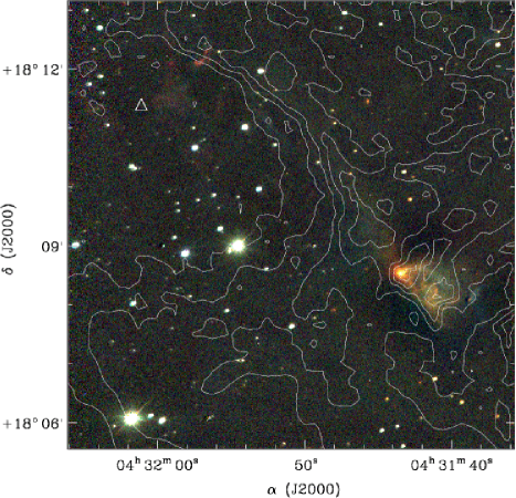
Figure 15.— Deep $JHK$ composite image of the L1551 NE region overlaid with contours of ¹³CO emission integrated from 6.5–7.9 km s^-1 (LSR). The linear stretch on all NIR bands is from $-\sigma$ to $20\sigma$, where $\sigma$ is the rms of the image, and the contour levels are $(n+2)$ K km s^-1, where $n$ is an integer. L1551 NE is the red source to the lower right in the image and the position of HH 262 is labeled (white triangle).

In Figure 15, our deep NIR imaging is shown as a $JHK$ composite image overlaid with ¹³CO contours. NIR nebulosity on the southwest side of L1551 NE is conical with an opening angle of $\sim 60^{\circ}$ and is symmetric with the jet axis of $\sim 243^{\circ}$ (Devine et al. 1999; Reipurth et al. 2000). On the northeast side, the nebulosity follows the parabolic shape of the ¹³CO emission and is brighter along the northern arm. This nebulosity extends from the L1551 NE source position and has a geometry that implies alignment with the jet axis.

HH 262 lies within the northeast cavity and has components with a wide range of radial velocities and proper motions suggesting that the jets from both L1551 IRS5 and L1551 NE may be interacting with this region (Devine et al. 1999; López et al. 1998). Faint $K$-band emission seen $\sim 1^{\prime}\!.5$ to the northwest of the nominal HH 262 position in Figure 15 is likely due to shocked H₂ associated with GH 9 (Graham & Heyer 1990; López et al. 1998). HH 286 lies further out of the L1551 cloud and also originates from either L1551 IRS5 or L1551 NE (Devine et al. 1999). The red lobe of the L1551 IRS5 molecular outflow overlaps with the northeast cavity (see Stojimirović et al. 2006, Figure 7), but the axis of that flow lies along the northern arm of the cavity making L1551 IRS5 unlikely responsible for excavating the mass from the northeast cavity.

We therefore attribute the northeast cavity feature to L1551 NE while, similar to the blue lobe of the L1551 IRS5 outflow, it contains features from both L1551 IRS5 and L1551 NE (Devine et al. 1999). The dynamical time for the northeast cavity based on its projected size and a velocity spread of $\sim 3$ km s^-1 is $\sim 10^{\rm 4-5}$ years. The mass of gas excavated from the region is estimated to be 2–3 $M_{\odot}$ from the deficit of ¹³CO and $A_{V}$ in the cavity relative to the average column depth of the cloud around the cavity.

6.3. The XZ/HL Tau Region

The XZ/HL Tau region is highly active (Mundt et al. 1990). XZ Tau is known to have poorly collimated outbursts on several year timescales (Krist et al. 1999), and a limb-brightened shell of ¹³CO is centered roughly on its position (Welch et al. 2000). In Figures 12(a) and (e) the acceleration of the ambient gas from around XZ/HL Tau is clearly evident. There is also a circular region devoid of ¹³CO emission in channel map (a) centered on the position of LkH$\alpha$ 358 that may be evidence for a weak wind.

The expanding half shell seen by Welch et al. (2000) is evident in channel maps (a) and (e) and extends to the position of HH 30 IRS in map (f). Also in Figure 12(f) there are two arcs curving around the east side of XZ Tau that are disjoint from the lower rim of the XZ Tau shell. The near one is smooth and filamentary, and the far one is clumpy. These features persist for multiple channels and move in unison away from the XZ/HL Tau region with decreasing velocity. This is consistent with gas expanding into the ambient cloud as it is accelerated from the XZ/HL Tau region. The expansion velocity is $\sim 0.7$ km s^-1 and the expansion age is $\lesssim 10^{5}$ years assuming this scenario. A simple estimate for the time between the ejection events is $\sim 10^{4}$ years. It is possible that these are molecular signatures of episodic outbursts similar to those seen in visible light (Coffey et al. 2004; Krist et al. 1999).

On the blueshifted side of the ¹³CO line core in Figures 12(a) and (b) a peculiar linear feature located $\sim 2^{\prime}$ east of XZ Tau extends in a northeast-southwest direction . This feature persists over $\sim 2$ km s^-1 and does not vary in position over those velocities. Figure 16 shows a composite $JHK$ image of the XZ/HL Tau region overlaid with ¹³CO contours. This linear feature seen in ¹³CO coincides with NIR nebulosity of the same morphology that is likely due to reflected light from XZ/HL Tau. This linear feature is also visible in H$\alpha$ emission (Devine et al. 1999), and likely delineates the rim of the cavity vacated by the energetics from XZ Tau, HL Tau, and HH 30 IRS (see Mundt et al. 1990).

Figure 16.— Same as Figure 15, but for the XZ/HL Tau region. The ¹³CO map has been integrated over velocities between 5.4 and 7.7 km s^-1 and the contour levels are $(5+1.5n)$ K km s^-1.

The ¹³CO emission shown in Figure 16 also traces well other diffuse NIR nebulosity. The nebulosity immediately below XZ Tau and the nebulosity stretching northward from HL Tau also may be delineating a boundary between high and low extinction regions in L1551. Unfortunately, not enough background stars are seen in our deep NIR images to do an extinction analysis in this region. However, these data are consistent with the interpretation of Welch et al. (2000) that the HL Tau lies at the boundary of a region excavated by XZ Tau.

Stars in this region of L1551 must have destroyed part of the cloud both to expose XZ Tau along our line of sight and to create the features seen in ¹³CO and the NIR. However, the modest diminution of ¹³CO column depth seen in our figures translate to only $\sim 0.1$ $M_{\odot}$ of excavated matter from the XZ/HL Tau region.

6.4. Summary of Stellar Feedback

A number of new features are revealed in our high-resolution maps that show clear signs of interaction between outflow from young stars and the ambient cloud from which they formed. The ¹³CO line wing emission traces the interaction between gas accelerated by embedded sources and the ambient cloud. At our sensitivity limit, this emission does not extend to velocities much beyond the escape velocity of the cloud and is therefore a good tracer of the energy that will remain in the cloud and ultimately contribute to its turbulent velocity field.

Using the closely Gaussian C¹⁸O composite spectrum to characterize the quiescent gas, the ¹³CO line wings are defined as $V_{\rm red}>7.5$ km s^-1, and $V_{\rm blue}<5.9$ km s^-1 (LSR). The energy in the red and blue wings are $\sim 1.5$ and $2.0\times 10^{44}$ ergs, respectively. If isotropy of outflow motion is assumed, the total energy in the ¹³CO line wings becomes $\sim 10^{45}$ ergs.

This is about a factor of 5 lower than recent estimates for the total outflow energy in L1551 using ¹²CO (Stojimirović et al. 2006) which traces both the bound and unbound outflow gas. All major outflow regions show clear evidence that gas is being accelerated beyond the gravitational confines of the cloud, and at least 4–5 $M_{\odot}$ of mass has been excavated from L1551 by the present day embedded stars. This suggests that L1551 was more massive at the inception of star formation by perhaps 60%.

7. Turbulence

While our ¹³CO data show a wealth of structure in the line wings due to the energetics from young embedded sources, the C¹⁸O emission has a closely Gaussian profile at our sensitivity level and is optically thin throughout the map. The C¹⁸O emission is thus better suited to probe the turbulent velocity and density fields in L1551.

The one-dimensional velocity dispersion of the composite C¹⁸O spectrum is 0.31 km s^-1. Subtracting in quadrature the thermal contribution to the measured width using Equation 6 with $\bar{m}=30\,m_{\rm H}$ and then multiplying by $\sqrt{3}$, the three-dimensional turbulent velocity dispersion $\sigma_{\rm turb}=0.52$ km s^-1. The total turbulent energy in L1551 is estimated to be $1/2M_{\rm tot}\sigma_{\rm turb}^{2}=4.3\times 10^{44}$ ergs, and $E_{\rm turb}\approx 0.4\,E_{\rm grav}$.

7.1. Spectrum of Fluctuations

A complete statistical description of fully developed turbulence is obtained in the scaling relations of the density and velocity fields. Under ideal circumstances, energy is conserved as it cascades from large to small scales at a rate proportional to $v^{3}(L)/L$, implying a self-similar velocity dispersion that scales as $v(L)\propto L^{\gamma}$, with $\gamma=1/3$ (Kolmogorov 1941). This line width-size relation translates to an energy spectrum $E(k)\propto k^{-\beta}$, with $\beta=5/3$, and a power spectrum of $P_{\rm v}(k)\propto k^{n}$, with $n={-(\beta+D-1)}$ and $D$ being the number of dimensions that the power spectrum is computed over. Other turbulence models, such as shock dominated (Burgers 1974) and multi-fractal (Boldyrev et al. 2002), also show distinct scaling relations.

Unfortunately, observers can only measure two dimensional distributions of velocity and density on the plane of the sky, and many different techniques are used to deduce the three-dimensional distributions from the available information. Line widths and velocity centroids are a direct measure of the velocity field and have been used widely to infer the characteristics of the underlying turbulence (e.g., Larson 1981; Scalo 1984; Dickman & Kleiner 1985; Kleiner & Dickman 1985; Miesch & Bally 1994). Other methods including the spectral correlation function (SCF; Rosolowsky et al. 1999), principle component analysis (PCA; Brunt & Heyer 2002), $\Delta$-variance (Stutzki et al. 1998), and velocity channel analysis (VCA; Lazarian & Pogosyan 2000, 2004) have had varying degrees of success.

7.1.1 Velocity Channel Analysis

Density and velocity fluctuations are not independent within the framework of homogeneous, isotropic turbulence and can theoretically be discerned through observation. The velocity channel analysis (VCA) technique has been developed toward this end (Lazarian & Pogosyan 2000, 2004) and has been used to successfully separate the velocity and density contributions to the power spectrum of H i in the Small Magellanic Cloud (Stanimirović & Lazarian 2001).

The intensity fluctuations within a spectral line map integrated over the full extent of the line profile are dominated by the density fluctuations such that the index of the two-dimensional power spectrum of intensity fluctuations equals the index of the three-dimensional density power spectrum

$$P_{\rho}^{2D,{\rm thick}}(k)\propto P_{\rho}^{3D}(k)\propto k^{n}$$ (7)

Intensity fluctuations within a thin slice in velocity space have contributions from both the velocity and density fluctuations in proportions that depends on the steepness of the three-dimensional density spectrum

$$P_{\rho}^{2D,{\rm thin}}(k)\propto\begin{cases}k^{n+\alpha/2}&:\quad n>-3\\ k^{-3+\alpha/2}&:\quad n<-3\\ \end{cases}$$ (8)

Here $\alpha$ is the power-law index of the second-order velocity structure function (see § 7.1.3). The formal criterion for a slice to be thin is that the dispersion of turbulent velocities on the scales studied be larger than the velocity slice thickness. The thin slice regime is not attainable for sub-sonic turbulence.

Figure 17.— The annular average of the two dimensional density power spectrum of C¹⁸O emission as a function of wave number. The corresponding scale in the map is plotted on the upper axis. The best fit power-law slope for $P_{\rho}^{\rm 2D}(k)$ is $-2.8$ and is shown as the line traversing the data.

Figure 17 shows the power spectrum of the velocity integrated C¹⁸O within the high-resolution region outlined with the dashed line in Figure 10. The velocity integrated map was first buffered on all sides with zeros to minimize aliasing effects and was then Fourier transformed using a Fast Fourier Transform (FFT) algorithm and squared. Circular annuli are averaged to obtain the mean value of the power spectrum in each annulus, and the dispersion of values within each annulus determine the error bars.

Figure 18.— The derived power-law index for $P_{\rho}^{2D}(k)$, the two-dimensional power spectrum of density fluctuations, as a function of the velocity width of the integrated map. The decrease in index as a function of increasing velocity width is expected, and the flattening out at large $\Delta v$ signifies the density dominated regime.

The power spectrum of Figure 17 follows a power-law form over the full range of scales sampled. A non-linear least squares fit to the power spectrum returns a slope of $n=-2.8\pm 0.1$, characterizing the density fluctuations as “shallow,” $n>-3$. The error here is derived from the variance of power spectrum indices fit to subsets of the C¹⁸O data.

Figure 18 shows the slope of the two-dimensional power spectrum as a function of velocity width. For each width, $\Delta v$, the C¹⁸O map was integrated in velocity across the necessary number of channels centered around the central channel in the line profile, $V_{\rm LSR}=6.7$ km s^-1. A power spectrum was then obtained in the same manner as described above. Shifting the window of channels by a single channel width in both directions gives two more measurements of the slope. The mean of the three values for $n_{\rm 2D}$ is represented as a filled circle in Figure 18 and the spread in these three values determines the error bar.

As the channel width increases, the slope of the two-dimensional power spectrum monotonically decreases. This is the behavior predicted by the VCA analysis. The trend levels out for channel widths greater than $\sim 0.6$ km s^-1 and likely signifies the transition into the density dominated regime. There is no sign of this trend tapering off for small $\Delta v$ and it is possible that this trend will continue to the thermal width of the C¹⁸O line, 0.06 km s^-1 (Lazarian, A. 2006, private communication).

Assuming that the value of $n_{\rm 2D}=-2.44$ is representative of the slope of $P_{\rho}^{2D}(k)$ in the thin regime, a value for the velocity spectrum index can be attained using Equation 8, $\alpha=0.72\pm 0.1$. This implies a three-dimensional power spectrum of velocity fluctuations, $P_{\rm v}^{3D}(k)\propto k^{-3.72}$, near the value predicted by the Kolmogorov formalism, $-11/3$.

7.1.2 Line Width-Size Relationship

The VCA results imply an energy spectrum index, $\beta=1.72$ and a line width-size index of $\gamma=0.36$. The line width size relationship for our C¹⁸O data are shown in Figure 19. The one-dimensional line widths in Figure 19 are computed by taking an intensity weighted average of all independent pixels in the C¹⁸O map downgraded in resolution to scale $L$. The average line width is then corrected for cloud depth effects by subtracting the dispersion in line centroids at the given map resolution (see Ossenkopf & Mac Low 2002). The derived trend in line width is characterized by $\gamma=0.07\pm 0.01$.

Figure 19.— The line width-size relation of the C¹⁸O gas in L1551. The sound speed for molecular gas with solar helium abundance at a kinetic temperature of 15 K is shown with the arrow.

This derivation of the line width-size relationship is fundamentally different than the standard method used where regions are identified as individual clouds or cores based on prescribed criteria and their sizes and line widths are then determined for each separate region (e.g., Larson 1981; Solomon et al. 1987; Fuller & Myers 1992). The observed power-law form of the line width-size relationship is generally thought to arise from interstellar turbulence (e.g., Larson 1981), but the relationship formed in this manner does not contain any direct information regarding the nature of turbulence within individual clouds.

In L1551, the line width-size relationship is very shallow. This result is inconsistent with the results from the VCA analysis assuming that the turbulence is homogeneous and isotropic. However, the derived line width-size relationship implies straightforwardly that the observed line widths are originating on small spatial scales which may indicate the presence of ongoing feedback (Nakamura et al. 2006).

7.1.3 The Structure Function

The velocity structure function measures velocity differences as a function of projected separation and is a common statistic used to characterize turbulent motions (e.g., Miesch & Bally 1994; Brunt & Heyer 2002; Esquivel & Lazarian 2005). For homogeneous, isotropic turbulence, the structure function is expected to follow a power-law form, $S_{\rm v}(\mbox{\boldmath$\tau$})\propto|\mbox{\boldmath$\tau$}|^{\alpha}$. The index, $\alpha$ is related to the index of the energy spectrum and line width-size relation, $\alpha=\beta-1$ and $\alpha=2\gamma$.

The form of the second-order velocity structure function is

$$S_{\rm v}(\mbox{\boldmath$\tau$})=\sum\langle\left[v_{\rm c}(\mbox{\boldmath$r$})-v_{\rm c}(\mbox{\boldmath$r$}+\mbox{\boldmath$\tau$})\right]^{2}\rangle,$$ (9)

where the position, $r$, and lag (i.e., projected separation), $\tau$, are two-dimensional functions on the plane of the sky, and the angled brackets signify an average over all pairs. The velocity centroid is

$$v_{\rm c}(\mbox{\boldmath$r$})=\frac{\sum T(\mbox{\boldmath$r$},v)v(\mbox{\boldmath$r$})}{\sum T(\mbox{\boldmath$r$},v)},$$ (10)

where $T$ is the antenna temperature and the sum is over velocity. The structure function of Equation 9 normalized by the variance of velocity centroids across the map,

$$\sigma_{\rm c}^{2}=\frac{\sum\left[v_{\rm c}(\mbox{\boldmath$r$})-\mu\right]^{2}}{N},$$ (11)

is denoted $S_{\rm v}^{*}(\mbox{\boldmath$\tau$})$, where $N$ is the number of pixels in the sum and

$$\mu=\frac{\sum v_{\rm c}}{N}$$ (12)

is the mean velocity centroid of the map. The normalized structure function has an algebraic relationship to the spatial autocorrelation function and approaches values of 2 for uncorrelated spectra (see Miesch & Bally 1994).

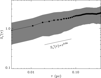
Figure 20.— Normalized second-order velocity structure function of the C¹⁸O emission in L1551 within the high-resolution region outlined in Figure 10. The gray shaded region indicates the allowed values of $S_{\rm v}^{*}(\tau)$ within the computed error estimates. The best power-law fit for $\tau<0.2$ pc is shown.

Detailed numerical tests have shown that the velocity structure function can be successfully used to retrieve the scaling properties of a three-dimensional velocity field from a data cube of position-position-velocity for turbulence with sonic Mach number $M_{s}\leq 2.5$ and in regions that are not dominated by density fluctuations (Brunt & Heyer 2002; Esquivel & Lazarian 2005). A straightforward way to compare the relative importance of the density fluctuations is through the second order density structure function.

$$S_{\rho}(\mbox{\boldmath$\tau$})=\sigma_{\rm v}^{2}\sum\langle\left[I(\mbox{\boldmath$r$})-I(\mbox{\boldmath$r$}+\mbox{\boldmath$\tau$})\right]^{2}\rangle,$$ (13)

where

$$I(\mbox{\boldmath$r$})=\sum T(\mbox{\boldmath$r$},v).$$ (14)

The sum in Equation 14 is over velocity, and $\sigma_{\rm v}$ is the velocity dispersion of the gas. To directly compare Equation 9 and Equation 13, “unnormalized” velocity centroids,

$$\tilde{v}_{\rm c}(\mbox{\boldmath$r$})=\sum T(\mbox{\boldmath$r$},v)v(\mbox{\boldmath$r$}),$$ (15)

replace the velocity centroids of Equation 9. The structure function of the unnormalized velocity centroids is denoted $\tilde{S}_{\rm v}(\tau)$, and it has been determined by numerical simulation that the velocity structure function accurately traces the turbulent velocity statistics for $\tilde{S}_{\rm v}(\mbox{\boldmath$\tau$})\gg S_{\rho}(\mbox{\boldmath$\tau$})$ (Esquivel & Lazarian 2005).

A value for the velocity centroid was computed at each independent pixel according to Equation 10. Only channels with signal greater than 2.5 $\sigma$ within the full width between first nulls of the composite spectrum were chosen as part of the sum, and only spectra with 3 or more channels meeting this criterion were considered, the rest were masked. The normalized structure function, $S_{\rm v}^{*}(\mbox{\boldmath$\tau$})$, is then computed using $\mu=6.69$ km s^-1 and $\sigma_{\rm c}=0.13$ km s^-1. A noise correction for $\sigma_{\rm c}$ (Miesch & Bally 1994) has negligible effect. The dispersion in centroid values at a given lag is used as the error estimate in $S_{\rm v}^{*}$ at that lag.

Figure 20 shows $S_{\rm v}^{*}(\tau)$ computed for C¹⁸O over the high resolution region of Figure 10. There is a shallow, increasing slope for $\tau\lesssim 0.2$ pc. A power-law fit to $S_{\rm v}^{*}(\tau)$ in this region yields a slope of $0.24\pm 0.01$. The function $\tilde{S}_{\rm v}(\tau)$, computed according to Equations 9 and 15 has amplitudes much greater than $S_{\rho}(\tau)$ everywhere in our map implying that density fluctuations do not dominate on any scale.

7.1.4 Discussion

The values of $\alpha$ derived from the VCA analysis, the line width-size relationship, and the second-order velocity structure function are, $0.72\pm 0.1$, $0.14\pm 0.02$, and $0.24\pm 0.01$, respectively. These values differ significantly according to the stated errors, but systematic errors may be important.

The VCA analysis is sensitive to gas temperature (Lazarian, A. 2006, private communication), and therefore varying kinetic temperatures throughout the cloud could confuse the VCA results. Gas temperatures are observed to vary between 9 and 25 K. Additionally, the slope of the two-dimensional power spectrum for a thin slice derived from Figure 18 is only a lower limit, since the trend toward larger slope indices may continue to smaller velocity widths than we have sampled with our data. However, a larger power spectrum index would only make the derived $\alpha$ values larger, and hence more discrepant.

The distribution of $S_{\rm v}^{*}(\tau)$ values at each $\tau$ is skewed due to the full spread in values being of order the mean at most lags. Using the median instead of the mean steepens the slope considerably to $\alpha=0.47\pm 0.02$. However, this still does not reconcile the disparate derived values for $\alpha$.

Lastly, the consistency of these analyses depends upon the turbulence being homogeneous and isotropic. The structure seen in the ¹³CO line wings in § 6 suggests that the energy input into the L1551 cloud is neither homogeneous nor isotropic, and it is not clear if this is a sound assumption for the turbulence in the cloud.

7.2. The Dissipation and Replenishment of Turbulent Energy

The total turbulent energy in L1551 is a substantial fraction of the gravitational energy. However, turbulent energy dissipates on short timescales (Stone et al. 1998; Mac Low & Klessen 2004) suggesting that the observed turbulence in L1551 is not primordial.

Galactic shear is negligible at the galactocentric distance of L1551 given its size, and no evidence of large scale rotation is seen in the first moment map of ¹³CO emission. There are no signs of recent supernova explosions in the proximity of L1551, nor are there H ii regions nearby. The ¹³CO line wings show coherent, thin structures that are expected at the early time evolution of supersonic turbulence (e.g., Porter et al. 1992). This structure is not random, but is clearly associated with the young stars in the region.

The total energy in the ¹³CO line wings estimated in § 6.4 is $4$–$10\times 10^{44}$ ergs. Both the dynamical timescale (§ 6) and and the diffusion timescale (§ 5.3.2) for the line wing features are $\sim 10^{5}$ years, and the age of the L1551 IRS5 outflow has been estimated to be the same order of magnitude (Moriarty-Schieven & Snell 1988; Richer et al. 2000). Therefore the observed energy in the cloud has been injected over the past $\sim 10^{5}$ years, and the observed rate of energy input into L1551 is $\dot{E}_{\rm input}\approx 2\times 10^{32}$ ergs s^-1, or 0.05 $L_{\odot}$.

Figure 21.— Intensity power spectra for the integrated intensity in the red (upper) and blue (lower) line wings of the ¹³CO emission. The power spectrum of the blue line wing is divided by 100 for viewing purposes. The velocity intervals for the integrated intensity are 7.5–9.0 km s^-1 and 3.4–5.7 km s^-1 for the red and blue line wing data, respectively. Clear excursions from the overall power-law form (lines) are seen near 1′ scales.

The energy from stellar feedback is expected to be highly turbulent and therefore the turbulent dissipation timescale, $t_{\rm diss}=E_{\rm turb}/\dot{E}_{\rm diss}$, sets the rate at which this energy is lost from the cloud. The dissipation of turbulent energy depends on the scale at which that turbulence is driven (Mac Low 1999; Stone et al. 1998; Gammie & Ostriker 1996). Figure 21 shows the power spectra of the integrated ¹³CO intensity in the red and blue line wings. The overall best fit for a single power law is shown as the thin lines. The slopes of these spectra are more shallow than the slopes in the line core, and there are also clear deviations from the linear trend at scales $\sim 1$′. Since the structures that are clearly associated with embedded sources dominate the emission in the line wings, the broad excess peaks in the line wing power spectra signify a preferential scale at which energy is being injected into the cloud.

Using the dispersion of the composite C¹⁸O spectrum, $0.31$ km s^-1, we estimate the flow crossing time at an energy injection scale of $0.05$ pc, $t_{\rm f}(\lambda_{\rm peak})\approx 0.1$ Myr. This timescale sets the overall scaling for $t_{\rm diss}$. In the numerical studies by Stone et al. (1998), $t_{\rm diss}$ was found to vary between $\sim 0.5$–0.8 $t_{\rm f}$ for a range in magnetic field strength between 0 and $\sim 50$ $\mu$G using a kinetic temperature of 15 K and a particle density equal to $\langle n\rangle\approx 10^{3}$ cm^-3. For $t_{\rm diss}=0.7\,t_{\rm f}$ and $E_{\rm turb}=4.3\times 10^{44}$ ergs, the turbulent energy dissipation rate in L1551 is $\dot{E}_{\rm diss}\approx 2\times 10^{32}$ ergs s^-1, approximately equal to the estimated energy input rate from outflow. Using Equation 7 from Mac Low (1999) with the appropriate input values gives a consistent number for $\dot{E}_{\rm diss}$.

The uncertainty in the stellar feedback energy is roughly a factor of 2 and the timescale over which the observed energy in outflow has been injected into the cloud is accurate to roughly the same level. The turbulent energy figure is relatively accurate, but our derived dissipation timescale may be off by a factor of 2 or more based on the broadness of the peaks seen in Figure 21 and the uncertain magnetic field strength in L1551 (see § 8). Therefore we can only conclude that $\dot{E}_{\rm diss}\approx\dot{E}_{\rm input}$ to order of magnitude. However, this rough agreement between energy rates along with the lack of evidence for any other form of energy input, the age of L1551 being several dynamical times, and the fact that turbulent energy only survives for roughly a flow crossing time, strongly suggest that the observed turbulent energy has been supplied by outflows from forming stars.

8. Discussion

The evolution of the L1551 cloud is influenced significantly by the stars forming within it. Ample evidence for energy injection and cloud destruction is apparent in our high-resolution maps. The observed turbulent motions in the cloud are short lived, $t_{\rm diss}\lesssim 0.1$ Myr, and exist primarily on small scales where they may act as a turbulent pressure to support the cloud against gravity (Bonazzola et al. 1992). Additionally, the energy input rate is estimated to be of the order of the dissipation rate. These calculations all support the idea that the progression of star formation is significantly influenced by the forming stars (e.g. Norman & Silk 1980; Li & Nakamura 2006).

The observed star formation efficiency, SFE, is defined as the present day stellar mass divided by the total present day mass in stars and gas. In L1551, ${\rm SFE}\approx 12$%. The total star formation efficiency, SFE_tot, is the fraction of total initial cloud mass that will ever become stars and may be as low as 9% in L1551 if the initial mass of the cloud were $\sim 1.6$ times the mass of the present day cloud. It appears that L1551 is not capable of producing significantly more stars in the future limiting SFE${}_{\rm tot}\lesssim 15$%. However, further study is needed in the high column regions to the northwest. The theoretical expectation of SFE_tot from outflow-regulated star formation is in the range 25–75% (Matzner & McKee 2000).

The age spread of PMS stars, fractional numbers of protostars, wTTSs, and cTTSs, and the spatial and kinematic distributions of the stellar component suggest L1551 has been forming stars for much longer than its present day dynamical time. The near equality of stellar feedback and turbulent dissipation provides a means for the cloud to stay close to virial equilibrium over its stellar production history (e.g., Tan et al. 2006; Krumholz 2006). However, the rate of star formation has not remained constant in L1551. Roughly 9 protostars have formed in L1551 in the past $\sim 0.1$ Myr. If this rate of star formation were projected backward in time even a few million years, the number of stars produced in L1551 would be in the hundreds. Therefore, we conclude that the increase in the rate of star formation over the lifetime of L1551 is robust. Evidence for accelerating star formation has been seen in Taurus as a whole (Palla & Stahler 2002) and in other well-studied star forming regions (Palla & Stahler 2000; Huff & Stahler 2006) and is expected if the star formation rate follows the dynamical rate of a contacting cloud (Palla & Stahler 1999).

Accelerating star formation fits loosely within the framework of dynamical star formation (e.g., Elmegreen 2000). However, dynamical models typically neglect or discount the effects of stellar feedback. This is untenable in the case of L1551. The timescales of purely dynamical star formation, typically 1–$2\,t_{\rm dyn}$, also do not match our observations. Even in the likely case that the dynamical timescale of the initial cloud was longer than the present day estimation, clear evidence for the formation of another star or stellar system that has yet to form pushes the productivity lifetime of L1551 well beyond the limits of purely dynamical formation.

Missing from this picture of star formation is information regarding the magnetic field. Polarization measurements of background starlight in the periphery of L1551 reveal a magnetic field direction somewhat suggestively aligned with the L1551 IRS5 outflow direction. However, a sub-millimeter polarization measurement of the dusty clump around L1551 IRS5 suggests a field direction nearly perpendicular to the outflow axis (Vallée & Bastien 2000). And while a firm lower limit of $2\,\mu$G has been set for the magnetic field strength in L1551 via rotation measures of background extragalactic radio sources (Simonetti & Cordes 1986), useful constraints on the field strength are precluded without detailed information about the ionization state of the gas.

The relative importance of the magnetic field in determining the structure and evolution of L1551 is presently not clear. More detailed observations regarding the magnetic field strength and orientation in L1551 are necessary to compliment this and other work (e.g., Moriarty-Schieven et al. 2006; Stojimirović et al. 2006) and to assess the role of magnetic fields in the formation of stars (e.g., Shu et al. 1987; McKee 1989; Ciolek & Mouschovias 1993; Shu et al. 2004).

9. Conclusion

This article outlines an extensive observational case study of an active star-forming molecular cloud and its pre-main sequence association of stars. New, key observational additions to the study of this region include wide-field, high-resolution maps of ¹³CO$(1-0)$ and C¹⁸O$(1-0)$ created through the combination of single-dish and interferometric data; deep, wide-field, near-infrared imaging; Spitzer IRAC data; and the culling of 2MASS and literature data regarding the young stellar population in the region. These data shed light on the relationship between the diverse phenomena observed in L1551 and the progression of star formation in this cloud.

Within a $1.\!\!^{\circ}6$ radius of the C¹⁸O intensity weighted mean position of L1551, $4^{\rm h}31^{\rm m}24^{\rm s}$, $+18^{\circ}10^{\prime}00^{\prime\prime}\,\,(J2000)$, 35 PMS stars are selected to be part of the L1551 association. The distribution of spectral class and derived bolometric luminosities suggest that star formation began $\gtrsim 6$ Myr ago. The spatial and kinematic distribution of PMS stars are also consistent with a long star formation history. The relatively high current rate of star formation is clear evidence that the star formation rate has increased over the productivity lifetime of L1551, consistent with accelerated star formation scenarios. The star formation appears to be progressing east to west with individual sites of star formation likely occurring in regions of quiescent gas.

The L1551 cloud contains 160 $M_{\odot}$ of total mass as traced by dust extinction, factors of 1.4 to 2 higher than previous estimates from molecular emission. The discrepancies are likely due to the saturation of CO emission in high column regions and the destruction of CO in areas of low extinction. The dynamical timescale for the cloud, given the radial distribution of mass within its 0.9 pc radius, is $t_{\rm dyn}=1.1$ Myr. This is significantly shorter than the inferred age of L1551 based on its stellar component.

The composite C¹⁸O line width infers a total kinetic energy in the cloud in accord with virial equilibrium assumptions. The turbulent velocity field in L1551 produces a density power spectrum $P_{\rho}(k)\propto k^{-2.8}$. We derive an energy spectrum index $\beta\approx 1$–2, but the observed turbulent motions exist primarily on small scales as inferred directly from the line width-size relationship in the cloud. The decay timescale for this turbulent energy is short, $t_{\rm diss}\lesssim 0.1$ Myr and is not primordial in origin.

The high-resolution ¹³CO emission traces well the stellar feedback in the cloud. Thin, filamentary features in the line wings of the ¹³CO emission signify the interface between outflow and quiescent gas and are used to estimate the stellar feedback, $\dot{E}_{\rm input}\approx 0.05$ $L_{\odot}$. This is not the full mechanical luminosity of outflow in L1551, rather a significant fraction of outflow energy contributes to the destruction of the cloud or is otherwise lost to the greater interstellar medium. It is estimated that 4–5 $M_{\odot}$ of gas has been excavated from the cloud by the current generation of outflows. The preferred scale at which energy is injected into the cloud is $\lambda_{\rm peak}\approx 0.05$ pc, about a thirtieth of the diameter of the cloud as seen in dust extinction.

The dissipation rate of turbulence and the rate of energy injection from outflow balance according to our calculations. There are no other significant sources of energy seen in L1551, and therefore outflows provide a significant supply of kinetic energy and play an important role in the evolution of the cloud.

Table 1Pre-main Sequence Stars in L1551 Region

Name	$\alpha(J2000)$	$\delta(J2000)$	$d$ (arcmin)	Sp. Typ.	$J$	$H$	$K_{s}$	$\Delta\alpha$	$\Delta\delta$	R.V.	note
L1551 IRS 5 (A+B)	4:31:34.1	18:08:04.9	3.08	G-K	13.71	11.51	9.82	$\cdots$	$\cdots$	$\cdots$	EB
HH30 IRS	4:31:37.5	18:12:24.5	4.01	M0	15.18	14.24	13.34	$\cdots$	$\cdots$	$\cdots$	EC
LkH$\alpha$ 358	4:31:36.1	18:13:43.3	4.70	M5.5	12.79	10.92	9.69	$\cdots$	$\cdots$	$\cdots$	E
L1551 NE (A+B)	4:31:44.4	18:08:31.5	5.07	$\cdots$	16.61	13.63	11.41	$\cdots$	$\cdots$	$\cdots$	EB
HL Tau	4:31:38.4	18:13:57.7	5.23	K7	10.62	9.17	7.41	-0.3	-2.1	$\cdots$	EC
XZ Tau A	4:31:40.1	18:13:57.2	5.50	M3	9.39	8.15	7.29	1.1	-1.9	$\cdots$	EB
XZ Tau B	4:31:40.1	18:13:57.2	5.50	M1.5	$\cdots$	$\cdots$	$\cdots$	$\cdots$	$\cdots$	$\cdots$	EB
MHO 4	4:31:24.1	18:00:21.5	9.64	M6	11.65	10.92	10.57	$\cdots$	$\cdots$	$\cdots$	$\cdots$
MHO 9	4:31:15.8	18:20:07.2	10.31	M4	11.21	10.55	10.30	$\cdots$	$\cdots$	$\cdots$	$\cdots$
MHO 5	4:32:16.1	18:12:46.4	12.68	M6	11.07	10.39	10.06	$\cdots$	$\cdots$	$\cdots$	$\cdots$
V 710 Tau B	4:31:57.8	18:21:35.1	14.09	M3	10.20	9.23	8.82	$\cdots$	$\cdots$	6.73	BC
V 710 Tau A	4:31:57.8	18:21:38.1	14.13	M1	9.82	9.06	8.69	1.5	-0.6	7.33	BC
V 826 Tau	4:32:15.8	18:01:38.7	14.88	K7	9.07	8.43	8.25	1.3	-2.2	4.43	B
V 827 Tau	4:32:14.6	18:20:14.7	15.79	K7	9.17	8.49	8.23	0.8	-1.5	4.63	$\cdots$
L1551-51	4:32:09.3	17:57:22.8	16.59	K7	9.70	9.06	8.85	1.1	-1.8	5.43	$\cdots$
TAP 44	4:32:37.7	18:06:36.6	17.83	$\cdots$	14.22	13.83	13.72	$\cdots$	$\cdots$	$\cdots$	$\cdots$
RX J0432.6+1809	4:32:41.1	18:09:23.9	18.32	M5	11.31	10.65	10.34	$\cdots$	$\cdots$	$\cdots$	$\cdots$
UX Tau A	4:30:04.0	18:13:49.4	19.38	K5	8.62	7.96	7.55	0.7	-1.4	2.23	B
UX Tau B	4:30:03.6	18:13:49.5	19.47	M2	9.87	8.95	8.92	$\cdots$	$\cdots$	4.63	BC
UX Tau C	4:30:03.6	18:13:49.5	19.47	M5	$\cdots$	$\cdots$	$\cdots$	$\cdots$	$\cdots$	1.33	B
L1551-55	4:32:43.7	18:02:56.3	20.21	K7	10.16	9.46	9.31	1.6	-1.3	4.73	$\cdots$
MHO 6	4:32:22.1	18:27:42.6	22.45	M5	11.71	11.02	10.65	$\cdots$	$\cdots$	$\cdots$	$\cdots$
MHO 7	4:32:26.3	18:27:52.1	23.19	M5	11.18	10.37	10.17	$\cdots$	$\cdots$	$\cdots$	$\cdots$
TAP 47	4:33:14.1	18:16:09.2	26.86	$\cdots$	9.62	9.11	8.95	$\cdots$	$\cdots$	$\cdots$	$\cdots$
DM Tau	4:33:48.7	18:10:10.0	34.37	M1	10.44	9.76	9.52	1.1	-1.9	3.53	$\cdots$
RX J0433.7+1823	4:33:42.0	18:24:27.4	35.81	G6	9.84	9.42	9.27	-1.3	-0.6	$\cdots$	M
HN Tau A	4:33:39.4	17:51:52.4	36.94	K5	10.82	9.49	8.44	1.5	-1.4	$\cdots$	$\cdots$
HN Tau B	4:33:39.4	17:51:52.4	36.94	M4	12.62	12.05	11.62	$\cdots$	$\cdots$	$\cdots$	$\cdots$
TAP 48	4:33:28.1	17:47:06.6	37.35	$\cdots$	12.69	12.36	12.24	$\cdots$	$\cdots$	$\cdots$	$\cdots$
RX J0432.8+1735	4:32:53.2	17:35:33.8	40.45	M2	10.00	9.23	9.02	0.8	-1.6	$\cdots$	$\cdots$
GG Tau Aa	4:32:30.4	17:31:40.6	41.45	K7	9.24	8.27	7.73	1.4	-2.0	4.23	B
GG Tau Ab	4:32:30.4	17:31:40.6	41.45	M0.5	10.12	9.07	8.53	$\cdots$	$\cdots$	$\cdots$	B
GG Tau Ba	4:32:30.3	17:31:30.3	41.60	M5	11.48	10.63	10.20	$\cdots$	$\cdots$	$\cdots$	B
GG Tau Bb	4:32:30.3	17:31:30.3	41.60	M7	13.16	12.38	12.01	$\cdots$	$\cdots$	$\cdots$	B
HBC 407	4:34:18.0	18:30:06.7	45.93	G8	10.58	10.08	9.90	0.0	-0.7	5.03	B
J2-2041	4:33:55.5	18:38:39.1	45.96	M3.5	10.53	9.87	9.61	1.0	-1.7	$\cdots$	$\cdots$
RX J0432.7+1853	4:32:42.4	18:55:10.2	48.84	K1	9.24	8.76	8.69	-0.5	-1.2	$\cdots$	$\cdots$
TAP 51	4:35:14.2	18:21:35.6	55.87	F8	9.32	9.00	8.92	0.0	-1.2	$\cdots$	$\cdots$
HBC 412	4:35:24.5	17:51:43.0	60.03	M2	10.03	9.33	9.08	$\cdots$	$\cdots$	7.33	B
HBC 388	4:27:10.6	17:50:42.6	63.26	K1	8.78	8.39	8.30	0.2	-1.5	1.63	B
HBC 392	4:31:27.2	17:06:24.9	63.59	K5	10.28	9.71	9.50	1.0	-2.8	3.13	B
RX J0433.5+1916	4:33:34.7	19:16:48.9	73.63	G6	10.96	10.52	10.40	0.3	-0.7	$\cdots$	$\cdots$
TAP 37	4:30:21.5	16:55:49.9	75.65	$\cdots$	14.38	14.19	13.91	$\cdots$	$\cdots$	$\cdots$	$\cdots$
RX J0437.5+1851	4:37:26.8	18:51:22.5	95.44	$\cdots$	9.97	8.76	9.07	$\cdots$	$\cdots$	$\cdots$	$\cdots$
RX J0437.4+1851A	4:37:26.9	18:51:26.8	95.49	K6	9.42	8.56	8.67	$\cdots$	$\cdots$	$\cdots$	BC
RX J0437.4+1851B	4:37:26.9	18:51:26.8	95.49	M0.5	$\cdots$	$\cdots$	$\cdots$	$\cdots$	$\cdots$	$\cdots$	B
TAP 33	4:22:53.0	17:34:15.8	126.73	$\cdots$	10.38	9.71	9.49	$\cdots$	$\cdots$	$\cdots$	S
TAP 53	4:36:10.8	16:04:52.5	142.66	$\cdots$	10.43	10.01	9.98	$\cdots$	$\cdots$	$\cdots$	S
RX J0431.4+2035	4:31:30.4	20:35:38.4	145.65	M4	10.97	10.31	10.10	$\cdots$	$\cdots$	$\cdots$	S
J2-157	4:20:52.7	17:46:41.5	151.92	M5.5	11.61	11.04	10.78	0.7	-1.5	$\cdots$	S
T Tau	4:21:59.4	19:32:06.4	156.79	K0	7.24	6.24	5.33	1.4	-1.2	5.73	BS
RX J0422.1+1934	4:22:05.0	19:34:48.3	157.09	M4.5	10.10	9.05	8.69	$\cdots$	$\cdots$	$\cdots$	S
TAP 38	4:31:13.8	20:53:43.6	163.74	$\cdots$	9.31	8.70	8.51	$\cdots$	$\cdots$	$\cdots$	S
RX J0438.2+2023	4:38:13.0	20:22:47.1	164.15	K2	10.07	9.53	9.36	$\cdots$	$\cdots$	$\cdots$	S
RX J0438.6+1546	4:38:39.1	15:46:13.7	177.46	K1	8.90	8.36	8.24	1.4	-1.9	$\cdots$	S
RX J0438.4+1543	4:38:27.7	15:43:38.0	178.01	K3	10.92	10.31	10.14	0.7	-1.1	$\cdots$	S
TAP 28	4:19:17.3	17:14:59.4	181.60	$\cdots$	9.96	9.36	9.18	$\cdots$	$\cdots$	$\cdots$	S
TAP 25	4:18:38.6	17:50:29.8	183.02	G0	8.34	8.26	8.16	$\cdots$	$\cdots$	$\cdots$	S
RX J0430.8+2113	4:30:49.2	21:14:10.6	184.36	G8	8.94	8.44	8.39	2.9	-2.8	$\cdots$	SM
HBC 376	4:18:51.7	17:23:16.6	185.09	K7	10.03	9.42	9.27	0.9	-1.5	4.63	S
RX J0423.7+1537	4:23:41.3	15:37:54.9	188.09	K2	9.41	8.93	8.81	0.8	-1.6	$\cdots$	S
HBC 372	4:18:21.5	16:58:47.0	199.62	K5	11.18	10.60	10.46	1.1	-1.4	2.43	S
RX J0444.4+1952	4:44:26.9	19:52:16.9	211.42	M1	9.56	8.88	8.71	-0.2	0.7	$\cdots$	SM
RX J0431.3+2150	4:31:16.9	21:50:25.3	220.43	K0	9.24	8.83	8.73	0.3	-1.4	$\cdots$	S
RX J0444.3+2017	4:44:23.6	20:17:17.5	223.75	K1	10.29	9.70	9.53	$\cdots$	$\cdots$	$\cdots$	S
RX J0443.4+1546	4:43:26.0	15:46:03.9	224.76	G7	10.71	10.20	10.10	0.2	-1.5	$\cdots$	S
DQ Tau	4:46:53.1	17:00:00.2	232.21	M0	9.51	8.54	7.98	0.0	-0.6	-17.37	VS
Haro 6-37	4:46:59.0	17:02:38.2	232.75	K6	9.24	7.99	7.31	0.0	-1.4	9.83	BS
Haro 6-37/c	4:46:59.0	17:02:38.2	232.75	K7	$\cdots$	$\cdots$	$\cdots$	$\cdots$	$\cdots$	6.13	BS
DR Tau	4:47:06.2	16:58:42.8	235.59	K7	8.85	7.80	6.87	0.5	-1.7	$\cdots$	S

References. — 1) Kenyon & Hartmann (1995); 2) Kenyon et al. (1998); 3) White & Ghez (2001); 4) Martín & Magazzù (1999); 5) Briceño et al. (1998); 6) Feigelson et al. (1987); 7) White et al. (1999); 8) Herbig & Bell (1995); 9) Gomez et al. (1992); 10) Wichmann et al. (2000); 11) Wichmann et al. (1996); 12) Basri & Marcy (1995); 13) Sartoretti et al. (1998)

Table 2Properties of Selected Pre-main Sequence Stars

Name	$T_{\rm eff}$ (K)	$L_{\rm bol}(L_{\odot})$	Type	Class	$A_{V}$	$J_{\rm c}$	age (Myr)	$M$ ($M_{\odot}$)
L1551 IRS 5 (A+B)	5000	21.6	proto	I	9.70	10.97	$0.1^{+0.9}_{-0.1}$	$\cdots$
HH30 IRS	3850	0.004	C	I/II	$\cdots$	15.18	$0.1^{+0.9}_{-0.1}$	$\cdots$
LkH$\alpha$ 358	3058	0.24	C	II	8.82	10.30	$0.1^{+0.9}_{-0.1}$	$\cdots$
L1551 NE (A+B)	$\cdots$	4.70	proto	0	$\cdots$	16.61	$0.1^{+0.9}_{-0.1}$	$\cdots$
HL Tau	4060	0.26	C	II	$\cdots$	10.62	$0.1^{+0.9}_{-0.1}$	$\cdots$
XZ Tau A	3415	1.24	C	II	3.07	8.52	$0.1^{+0.9}_{-0.1}$	$\cdots$
XZ Tau B	3633	0.05	C	$\cdots$	1.39	$\cdots$	$0.1^{+0.9}_{-0.1}$	$\cdots$
MHO 4	2990	0.08	W	$\cdots$	0.69	11.46	$1.0^{+0.8}_{-0.2}$	0.11
MHO 9	3270	0.18	W	$\cdots$	1.73	10.72	$4.0^{+0.5}_{-2.4}$	0.25
MHO 5	2990	0.12	C	II	0.11	11.04	$1.3^{+0.3}_{-0.3}$	0.17
V 710 Tau B	3560	0.63	W	II	1.82	8.47	$1.3^{+0.8}_{-0.3}$	0.62
V 710 Tau A	3705	0.51	C	II	1.80	8.77	$3.2^{+1.8}_{-0.9}$	0.80
V 826 Tau	4060	1.30	W	III	0.69	8.88	$2.8^{+2.2}_{-1.4}$	1.20
V 827 Tau	4060	1.33	W	III	1.14	8.85	$2.5^{+2.5}_{-0.7}$	1.20
L1551-51	4060	0.61	W	III	0.00	9.70	$6.4^{+2.7}_{-2.8}$	1.10
RX J0432.6+1809	3125	0.10	W	$\cdots$	0.00	11.31	$2.2^{+0.6}_{-0.8}$	0.20
UX Tau A	4350	1.93	C	II	0.26	8.55	$1.8^{+1.8}_{-0.8}$	1.40
UX Tau B	3560	0.19	W	III	0.26	9.80	$7.1^{+1.9}_{-3.1}$	0.57
UX Tau C	3125	0.10	W	$\cdots$	0.57	$\cdots$	$1.3^{+2.3}_{-0.3}$	0.13
L1551-55	4060	0.52	W	III	0.69	9.97	$8.9^{+3.7}_{-3.9}$	1.05
MHO 6	3125	0.08	W	$\cdots$	0.54	11.56	$2.8^{+1.2}_{-0.6}$	0.17
MHO 7	3125	0.11	W	$\cdots$	0.23	11.12	$1.6^{+0.9}_{-0.5}$	0.20
DM Tau	3705	0.33	C	II	0.00	10.44	$6.4^{+4.9}_{-2.4}$	0.70
HN Tau A	4350	0.49	C	II	2.79	10.03	$20.0^{+11.7}_{-7.3}$	1.05
HN Tau B	3270	0.03	C	$\cdots$	0.91	12.36	$11.4^{+8.8}_{-2.5}$	0.17
RX J0432.8+1735	3560	0.38	W	$\cdots$	0.00	10.00	$2.8^{+0.3}_{-1.3}$	0.62
GG Tau Aa	4060	1.52	C	II	1.90	8.70	$1.6^{+1.6}_{-0.6}$	1.20
GG Tau Ab	3778	0.82	C	II	3.01	9.27	$1.8^{+1.4}_{-0.6}$	0.90
GG Tau Ba	3125	0.11	C	II	1.12	11.16	$1.0^{+1.0}_{-0.1}$	0.13
GG Tau Bb	2880	0.02	C	II	0.63	12.98	$2.5^{+0.9}_{-0.5}$	0.05
HBC 407	5520	0.71	W	III	1.95	10.03	MS?	1.00
J2-2041	3343	0.25	W	III	0.90	10.28	$1.8^{+2.2}_{-0.1}$	0.30
RX J0432.7+1853	5080	1.23	W	$\cdots$	0.00	9.24	$22.4^{+22.6}_{-6.6}$	1.15
TAP 51	6200	2.08	W	$\cdots$	0.91	9.06	MS?	1.20
HBC 412	3560	0.37	W	III	0.00	10.03	$2.5^{+2.0}_{-0.9}$	0.57
HBC 388	5080	1.87	W	$\cdots$	0.00	8.78	$12.6^{+9.8}_{-1.5}$	1.40
HBC 392	4350	0.74	W	III	2.46	9.59	$12.6^{+1.6}_{-6.9}$	1.20

References. — 1) Kenyon & Hartmann (1995); 2) White & Ghez (2001); 3) Briceño et al. (1998); 4) Luhman (2000); 5) Gomez et al. (1992)

References

- Adams et al. (1987) Adams, F. C., Lada, C. J., & Shu, F. H. 1987, ApJ, 312, 788
- Bachiller (1996) Bachiller, R. 1996, ARA&A, 34, 111
- Ballesteros-Paredes et al. (1999) Ballesteros-Paredes, J., Hartmann, L., & Vázquez-Semadeni, E. 1999, ApJ, 527, 285
- Ballesteros-Paredes et al. (2007) Ballesteros-Paredes, J., Klessen, R. S., Mac Low, M.-M., & Vazquez-Semadeni, E. 2007, in Protostars and Planets V, ed. B. Reipurth, D. Jewitt, & K. Keil, 63–80
- Baraffe et al. (1998) Baraffe, I., Chabrier, G., Allard, F., & Hauschildt, P. H. 1998, A&A, 337, 403
- Baraffe et al. (2002) —. 2002, A&A, 382, 563
- Barsony et al. (1993) Barsony, M., Scoville, N. Z., & Chandler, C. J. 1993, ApJ, 409, 275
- Basri & Marcy (1995) Basri, G. & Marcy, G. W. 1995, AJ, 109, 762
- Beichman et al. (1986) Beichman, C. A., Myers, P. C., Emerson, J. P., Harris, S., Mathieu, R., Benson, P. J., & Jennings, R. E. 1986, ApJ, 307, 337
- Bertout et al. (1999) Bertout, C., Robichon, N., & Arenou, F. 1999, A&A, 352, 574
- Bessell (1991) Bessell, M. S. 1991, AJ, 101, 662
- Bloemen et al. (1986) Bloemen, J. B. G. M., Strong, A. W., Mayer-Hasselwander, H. A., Blitz, L., Cohen, R. S., Dame, T. M., Grabelsky, D. A., Thaddeus, P., Hermsen, W., & Lebrun, F. 1986, A&A, 154, 25
- Bohlin et al. (1978) Bohlin, R. C., Savage, B. D., & Drake, J. F. 1978, ApJ, 224, 132
- Boldyrev et al. (2002) Boldyrev, S., Nordlund, Å., & Padoan, P. 2002, Physical Review Letters, 89, 031102
- Bonazzola et al. (1992) Bonazzola, S., Perault, M., Puget, J. L., Heyvaerts, J., Falgarone, E., & Panis, J. F. 1992, Journal of Fluid Mechanics, 245, 1
- Briceño et al. (1998) Briceño, C., Hartmann, L., Stauffer, J., & Martín, E. 1998, AJ, 115, 2074
- Briceño et al. (2002) Briceño, C., Luhman, K. L., Hartmann, L., Stauffer, J. R., & Kirkpatrick, J. D. 2002, ApJ, 580, 317
- Brunt & Heyer (2002) Brunt, C. M. & Heyer, M. H. 2002, ApJ, 566, 276
- Burgers (1974) Burgers, J. M. 1974, The Nonlinear Diffusion Equation (Dordrecht: Reidel)
- Ciolek & Mouschovias (1993) Ciolek, G. E. & Mouschovias, T. C. 1993, ApJ, 418, 774
- Ciolek & Mouschovias (1994) —. 1994, ApJ, 425, 142
- Coffey et al. (2004) Coffey, D., Downes, T. P., & Ray, T. P. 2004, A&A, 419, 593
- Crutcher (1999) Crutcher, R. M. 1999, ApJ, 520, 706
- Cunningham et al. (2006) Cunningham, A. J., Frank, A., Quillen, A. C., & Blackman, E. G. 2006, ApJ, 653, 416
- Dame et al. (2001) Dame, T. M., Hartmann, D., & Thaddeus, P. 2001, ApJ, 547, 792
- Devine et al. (1999) Devine, D., Reipurth, B., & Bally, J. 1999, AJ, 118, 972
- Dickman (1978) Dickman, R. L. 1978, ApJS, 37, 407
- Dickman & Kleiner (1985) Dickman, R. L. & Kleiner, S. C. 1985, ApJ, 295, 479
- Draper et al. (1985) Draper, P. W., Warren-Smith, R. F., & Scarrott, S. M. 1985, MNRAS, 216, 7P
- Ducourant et al. (2005) Ducourant, C., Teixeira, R., Périé, J. P., Lecampion, J. F., Guibert, J., & Sartori, M. J. 2005, A&A, 438, 769
- Ekers & Rots (1979) Ekers, R. D. & Rots, A. H. 1979, in ASSL Vol. 76: IAU Colloq. 49: Image Formation from Coherence Functions in Astronomy, ed. C. van Schooneveld, 61–+
- Elmegreen (2000) Elmegreen, B. G. 2000, ApJ, 530, 277
- Elmegreen & Scalo (2004) Elmegreen, B. G. & Scalo, J. 2004, ARA&A, 42, 211
- Elston et al. (2003) Elston, R., Raines, S. N., Hanna, K. T., Hon, D. B., Julian, J., Horrobin, M., Harmer, C. F. W., & Epps, H. W. 2003, in Instrument Design and Performance for Optical/Infrared Ground-based Telescopes. Edited by Iye, Masanori; Moorwood, Alan F. M. Proceedings of the SPIE, Volume 4841, pp. 1611-1624 (2003)., ed. M. Iye & A. F. M. Moorwood, 1611–1624
- Esquivel & Lazarian (2005) Esquivel, A. & Lazarian, A. 2005, ApJ, 631, 320
- Fazio et al. (2004) Fazio, G. G., Hora, J. L., Allen, L. E., Ashby, M. L. N., Barmby, P., Deutsch, L. K., Huang, J.-S., Kleiner, S., Marengo, M., Megeath, S. T., Melnick, G. J., Pahre, M. A., Patten, B. M., Polizotti, J., Smith, H. A., Taylor, R. S., Wang, Z., Willner, S. P., Hoffmann, W. F., Pipher, J. L., Forrest, W. J., McMurty, C. W., McCreight, C. R., McKelvey, M. E., McMurray, R. E., Koch, D. G., Moseley, S. H., Arendt, R. G., Mentzell, J. E., Marx, C. T., Losch, P., Mayman, P., Eichhorn, W., Krebs, D., Jhabvala, M., Gezari, D. Y., Fixsen, D. J., Flores, J., Shakoorzadeh, K., Jungo, R., Hakun, C., Workman, L., Karpati, G., Kichak, R., Whitley, R., Mann, S., Tollestrup, E. V., Eisenhardt, P., Stern, D., Gorjian, V., Bhattacharya, B., Carey, S., Nelson, B. O., Glaccum, W. J., Lacy, M., Lowrance, P. J., Laine, S., Reach, W. T., Stauffer, J. A., Surace, J. A., Wilson, G., Wright, E. L., Hoffman, A., Domingo, G., & Cohen, M. 2004, ApJS, 154, 10
- Feigelson et al. (1987) Feigelson, E. D., Jackson, J. M., Mathieu, R. D., Myers, P. C., & Walter, F. M. 1987, AJ, 94, 1251
- Fuller & Myers (1992) Fuller, G. A. & Myers, P. C. 1992, ApJ, 384, 523
- Gammie & Ostriker (1996) Gammie, C. F. & Ostriker, E. C. 1996, ApJ, 466, 814
- Ghez et al. (1993) Ghez, A. M., Neugebauer, G., & Matthews, K. 1993, AJ, 106, 2005
- Giovanardi et al. (2000) Giovanardi, C., Rodríguez, L. F., Lizano, S., & Cantó, J. 2000, ApJ, 538, 728
- Gomez et al. (1992) Gomez, M., Jones, B. F., Hartmann, L., Kenyon, S. J., Stauffer, J. R., Hewett, R., & Reid, I. N. 1992, AJ, 104, 762
- Graham & Heyer (1990) Graham, J. A. & Heyer, M. H. 1990, PASP, 102, 972
- Hartigan et al. (1995) Hartigan, P., Edwards, S., & Ghandour, L. 1995, ApJ, 452, 736
- Hartmann (2001) Hartmann, L. 2001, AJ, 121, 1030
- Hartmann (2002) —. 2002, ApJ, 578, 914
- Hartmann et al. (2001) Hartmann, L., Ballesteros-Paredes, J., & Bergin, E. A. 2001, ApJ, 562, 852
- Hartmann et al. (1998) Hartmann, L., Calvet, N., Gullbring, E., & D’Alessio, P. 1998, ApJ, 495, 385
- Harvey et al. (2003) Harvey, D. W. A., Wilner, D. J., Lada, C. J., Myers, P. C., & Alves, J. F. 2003, ApJ, 598, 1112
- Hayashi (1961) Hayashi, C. 1961, PASJ, 13, 450
- Helfer et al. (2003) Helfer, T. T., Thornley, M. D., Regan, M. W., Wong, T., Sheth, K., Vogel, S. N., Blitz, L., & Bock, D. C.-J. 2003, ApJS, 145, 259
- Herbig & Bell (1995) Herbig, G. H. & Bell, K. R. 1995, VizieR Online Data Catalog, 5073, 0
- Holdaway (1999) Holdaway, M. A. 1999, in ASP Conf. Ser. 180: Synthesis Imaging in Radio Astronomy II, ed. G. B. Taylor, C. L. Carilli, & R. A. Perley, 401–+
- Huff & Stahler (2006) Huff, E. M. & Stahler, S. W. 2006, ApJ, 644, 355
- Jeans (1961) Jeans, J. H. 1961, Astronomy and cosmogony (New York: Dover, 1961)
- Kauffmann et al. (2005) Kauffmann, J., Bertoldi, F., Evans, II, N. J., & the C2D Collaboration. 2005, Astronomische Nachrichten, 326, 878
- Kenyon et al. (1998) Kenyon, S. J., Brown, D. I., Tout, C. A., & Berlind, P. 1998, AJ, 115, 2491
- Kenyon & Hartmann (1995) Kenyon, S. J. & Hartmann, L. 1995, ApJS, 101, 117
- Kleiner & Dickman (1985) Kleiner, S. C. & Dickman, R. L. 1985, ApJ, 295, 466
- Kohler & Leinert (1998) Kohler, R. & Leinert, C. 1998, A&A, 331, 977
- Kolmogorov (1941) Kolmogorov, A. N. 1941, Doklady Akad Nauk Minerologia USSR, 30, 301
- Krist et al. (1999) Krist, J. E., Stapelfeldt, K. R., Burrows, C. J., Hester, J. J., Watson, A. M., Ballester, G. E., Clarke, J. T., Crisp, D., Evans, R. W., Gallagher, III, J. S., Griffiths, R. E., Hoessel, J. G., Holtzman, J. A., Mould, J. R., Scowen, P. A., & Trauger, J. T. 1999, ApJ, 515, L35
- Krumholz (2006) Krumholz, M. R. 2006, ArXiv Astrophysics e-prints
- Krumholz & Tan (2007) Krumholz, M. R. & Tan, J. C. 2007, ApJ, 654, 304
- Lada (1987) Lada, C. J. 1987, in IAU Symp. 115: Star Forming Regions, ed. M. Peimbert & J. Jugaku, 1–17
- Lada (1991) Lada, C. J. 1991, in NATO ASIC Proc. 342: The Physics of Star Formation and Early Stellar Evolution, ed. C. J. Lada & N. D. Kylafis, 329–+
- Lada et al. (1994) Lada, C. J., Lada, E. A., Clemens, D. P., & Bally, J. 1994, ApJ, 429, 694
- Larson (1981) Larson, R. B. 1981, MNRAS, 194, 809
- Lazarian & Pogosyan (2000) Lazarian, A. & Pogosyan, D. 2000, ApJ, 537, 720
- Lazarian & Pogosyan (2004) —. 2004, ApJ, 616, 943
- Leinert et al. (1993) Leinert, C., Zinnecker, H., Weitzel, N., Christou, J., Ridgway, S. T., Jameson, R., Haas, M., & Lenzen, R. 1993, A&A, 278, 129
- Li & Nakamura (2006) Li, Z.-Y. & Nakamura, F. 2006, ApJ, 640, L187
- Lombardi & Alves (2001) Lombardi, M. & Alves, J. 2001, A&A, 377, 1023
- López et al. (1998) López, R., Rosado, M., Riera, A., Noriega-Crespo, A., Raga, A. C., Estalella, R., Anglada, G., Le Coarer, E., Langarica, R., Tinoco, S., & Cantó, J. 1998, AJ, 116, 845
- Luhman (2000) Luhman, K. L. 2000, ApJ, 544, 1044
- Luhman et al. (2003) Luhman, K. L., Stauffer, J. R., Muench, A. A., Rieke, G. H., Lada, E. A., Bouvier, J., & Lada, C. J. 2003, ApJ, 593, 1093
- Lynds (1962) Lynds, B. T. 1962, ApJS, 7, 1
- Mac Low (1999) Mac Low, M.-M. 1999, ApJ, 524, 169
- Mac Low & Klessen (2004) Mac Low, M.-M. & Klessen, R. S. 2004, Reviews of Modern Physics, 76, 125
- Martín & Magazzù (1999) Martín, E. L. & Magazzù, A. 1999, A&A, 342, 173
- Matzner & McKee (2000) Matzner, C. D. & McKee, C. F. 2000, ApJ, 545, 364
- McKee (1989) McKee, C. F. 1989, ApJ, 345, 782
- Meyer et al. (2000) Meyer, M. R., Adams, F. C., Hillenbrand, L. A., Carpenter, J. M., & Larson, R. B. 2000, Protostars and Planets IV, 121
- Meyer et al. (1997) Meyer, M. R., Calvet, N., & Hillenbrand, L. A. 1997, AJ, 114, 288
- Miesch & Bally (1994) Miesch, M. S. & Bally, J. 1994, ApJ, 429, 645
- Moriarty-Schieven et al. (1995) Moriarty-Schieven, G. H., Butner, H. M., & Wannier, P. G. 1995, ApJ, 445, L55
- Moriarty-Schieven et al. (2006) Moriarty-Schieven, G. H., Johnstone, D., Bally, J., & Jenness, T. 2006, ApJ, 645, 357
- Moriarty-Schieven & Snell (1988) Moriarty-Schieven, G. H. & Snell, R. L. 1988, ApJ, 332, 364
- Moriarty-Schieven et al. (1987) Moriarty-Schieven, G. H., Snell, R. L., Strom, S. E., Schloerb, F. P., Strom, K. M., & Grasdalen, G. L. 1987, ApJ, 319, 742
- Moriarty-Schieven & Wannier (1991) Moriarty-Schieven, G. H. & Wannier, P. G. 1991, ApJ, 373, L23
- Mundt et al. (1990) Mundt, R., Buehrke, T., Solf, J., Ray, T. P., & Raga, A. C. 1990, A&A, 232, 37
- Mundt & Fried (1983) Mundt, R. & Fried, J. W. 1983, ApJ, 274, L83
- Myers et al. (1983) Myers, P. C., Linke, R. A., & Benson, P. J. 1983, ApJ, 264, 517
- Nakamura et al. (2006) Nakamura, F., McKee, C. F., Klein, R. I., & Fisher, R. T. 2006, ApJS, 164, 477
- Norman & Silk (1980) Norman, C. & Silk, J. 1980, ApJ, 238, 158
- Ochsenbein et al. (2000) Ochsenbein, F., Bauer, P., & Marcout, J. 2000, A&AS, 143, 23
- Onishi et al. (1998) Onishi, T., Mizuno, A., Kawamura, A., Ogawa, H., & Fukui, Y. 1998, ApJ, 502, 296
- Ossenkopf & Mac Low (2002) Ossenkopf, V. & Mac Low, M.-M. 2002, A&A, 390, 307
- Padoan et al. (2001) Padoan, P., Juvela, M., Goodman, A. A., & Nordlund, Å. 2001, ApJ, 553, 227
- Padoan & Nordlund (2002) Padoan, P. & Nordlund, Å. 2002, ApJ, 576, 870
- Palla & Stahler (1999) Palla, F. & Stahler, S. W. 1999, ApJ, 525, 772
- Palla & Stahler (2000) —. 2000, ApJ, 540, 255
- Palla & Stahler (2002) —. 2002, ApJ, 581, 1194
- Porter et al. (1992) Porter, D. H., Pouquet, A., & Woodward, P. R. 1992, Physical Review Letters, 68, 3156
- Pound & Bally (1991) Pound, M. W. & Bally, J. 1991, ApJ, 383, 705
- Prantzos & Aubert (1995) Prantzos, N. & Aubert, O. 1995, A&A, 302, 69
- Quillen et al. (2005) Quillen, A. C., Thorndike, S. L., Cunningham, A., Frank, A., Gutermuth, R. A., Blackman, E. G., Pipher, J. L., & Ridge, N. 2005, ApJ, 632, 941
- Reid et al. (2001) Reid, I. N., Burgasser, A. J., Cruz, K. L., Kirkpatrick, J. D., & Gizis, J. E. 2001, AJ, 121, 1710
- Reipurth & Bally (2001) Reipurth, B. & Bally, J. 2001, ARA&A, 39, 403
- Reipurth et al. (2000) Reipurth, B., Yu, K. C., Heathcote, S., Bally, J., & Rodríguez, L. F. 2000, AJ, 120, 1449
- Reipurth & Zinnecker (1993) Reipurth, B. & Zinnecker, H. 1993, A&A, 278, 81
- Richer et al. (2000) Richer, J. S., Shepherd, D. S., Cabrit, S., Bachiller, R., & Churchwell, E. 2000, Protostars and Planets IV, 867
- Rieke & Lebofsky (1985) Rieke, G. H. & Lebofsky, M. J. 1985, ApJ, 288, 618
- Román-Zúñiga et al. (2006) Román-Zúñiga, C., Levine, J. L., Stolte, A., & Lada, E. A. 2006, in preparation
- Rosolowsky et al. (1999) Rosolowsky, E. W., Goodman, A. A., Wilner, D. J., & Williams, J. P. 1999, ApJ, 524, 887
- Sartoretti et al. (1998) Sartoretti, P., Brown, R. A., Latham, D. W., & Torres, G. 1998, A&A, 334, 592
- Sault et al. (1995) Sault, R. J., Teuben, P. J., & Wright, M. C. H. 1995, in Astronomical Society of the Pacific Conference Series, 433–+
- Scalo (1984) Scalo, J. M. 1984, ApJ, 277, 556
- Shu (1977) Shu, F. H. 1977, ApJ, 214, 488
- Shu et al. (1987) Shu, F. H., Adams, F. C., & Lizano, S. 1987, ARA&A, 25, 23
- Shu et al. (2004) Shu, F. H., Li, Z.-Y., & Allen, A. 2004, in ASP Conf. Ser. 323: Star Formation in the Interstellar Medium: In Honor of David Hollenbach, ed. D. Johnstone, F. C. Adams, D. N. C. Lin, D. A. Neufeeld, & E. C. Ostriker, 37–+
- Simon et al. (1995) Simon, M., Ghez, A. M., Leinert, C., Cassar, L., Chen, W. P., Howell, R. R., Jameson, R. F., Matthews, K., Neugebauer, G., & Richichi, A. 1995, ApJ, 443, 625
- Simonetti & Cordes (1986) Simonetti, J. H. & Cordes, J. M. 1986, ApJ, 303, 659
- Skrutskie et al. (2006) Skrutskie, M. F., Cutri, R. M., Stiening, R., Weinberg, M. D., Schneider, S., Carpenter, J. M., Beichman, C., Capps, R., Chester, T., Elias, J., Huchra, J., Liebert, J., Lonsdale, C., Monet, D. G., Price, S., Seitzer, P., Jarrett, T., Kirkpatrick, J. D., Gizis, J. E., Howard, E., Evans, T., Fowler, J., Fullmer, L., Hurt, R., Light, R., Kopan, E. L., Marsh, K. A., McCallon, H. L., Tam, R., Van Dyk, S., & Wheelock, S. 2006, AJ, 131, 1163
- Snell (1981) Snell, R. L. 1981, ApJS, 45, 121
- Snell et al. (1980) Snell, R. L., Loren, R. B., & Plambeck, R. L. 1980, ApJ, 239, L17
- Snell et al. (1984) Snell, R. L., Scoville, N. Z., Sanders, D. B., & Erickson, N. R. 1984, ApJ, 284, 176
- Solomon et al. (1987) Solomon, P. M., Rivolo, A. R., Barrett, J., & Yahil, A. 1987, ApJ, 319, 730
- Stanimirović & Lazarian (2001) Stanimirović, S. & Lazarian, A. 2001, ApJ, 551, L53
- Stanimirović et al. (1999) Stanimirović, S., Staveley-Smith, L., Dickey, J. M., Sault, R. J., & Snowden, S. L. 1999, MNRAS, 302, 417
- Steer et al. (1984) Steer, D. G., Dewdney, P. E., & Ito, M. R. 1984, A&A, 137, 159
- Stojimirović et al. (2006) Stojimirović, I., Narayanan, G., Snell, R. L., & Bally, J. 2006, ApJ, 649, 280
- Stone et al. (1998) Stone, J. M., Ostriker, E. C., & Gammie, C. F. 1998, ApJ, 508, L99
- Stutzki et al. (1998) Stutzki, J., Bensch, F., Heithausen, A., Ossenkopf, V., & Zielinsky, M. 1998, A&A, 336, 697
- Swift (2006) Swift, J. J. 2006, PhD thesis, University of California, Berkeley
- Swift et al. (2005) Swift, J. J., Welch, W. J., & Di Francesco, J. 2005, ApJ, 620, 823
- Swift et al. (2006) Swift, J. J., Welch, W. J., Di Francesco, J., & Stojimirović, I. 2006, ApJ, 637, 392
- Tan et al. (2006) Tan, J. C., Krumholz, M. R., & McKee, C. F. 2006, ApJ, 641, L121
- Vallée & Bastien (2000) Vallée, J. P. & Bastien, P. 2000, ApJ, 530, 806
- Vázquez-Semadeni et al. (2005) Vázquez-Semadeni, E., Kim, J., & Ballesteros-Paredes, J. 2005, ApJ, 630, L49
- Welch et al. (2000) Welch, W. J., Hartmann, L., Helfer, T., & Briceño, C. 2000, ApJ, 540, 362
- Welch et al. (1996) Welch, W. J., Thornton, D. D., Plambeck, R. L., Wright, M. C. H., Lugten, J., Urry, L., Fleming, M., Hoffman, W., Hudson, J., Lum, W. T., Forster, J. . R., Thatte, N., Zhang, X., Zivanovic, S., Snyder, L., Crutcher, R., Lo, K. Y., Wakker, B., Stupar, M., Sault, R., Miao, Y., Rao, R., Wan, K., Dickel, H. R., Blitz, L., Vogel, S. N., Mundy, L., Erickson, W., Teuben, P. J., Morgan, J., Helfer, T., Looney, L., de Gues, E., Grossman, A., Howe, J. E., Pound, M., & Regan, M. 1996, PASP, 108, 93
- White et al. (2000) White, G. J., Liseau, R., Men’shchikov, A. B., Justtanont, K., Nisini, B., Benedettini, M., Caux, E., Ceccarelli, C., Correia, J. C., Giannini, T., Kaufman, M., Lorenzetti, D., Molinari, S., Saraceno, P., Smith, H. A., Spinoglio, L., & Tommasi, E. 2000, A&A, 364, 741
- White & Ghez (2001) White, R. J. & Ghez, A. M. 2001, ApJ, 556, 265
- White et al. (1999) White, R. J., Ghez, A. M., Reid, I. N., & Schultz, G. 1999, ApJ, 520, 811
- Wichmann et al. (1996) Wichmann, R., Krautter, J., Schmitt, J. H. M. M., Neuhaeuser, R., Alcala, J. M., Zinnecker, H., Wagner, R. M., Mundt, R., & Sterzik, M. F. 1996, A&A, 312, 439
- Wichmann et al. (2000) Wichmann, R., Torres, G., Melo, C. H. F., Frink, S., Allain, S., Bouvier, J., Krautter, J., Covino, E., & Neuhäuser, R. 2000, A&A, 359, 181
- Yokogawa et al. (2003) Yokogawa, S., Kitamura, Y., Momose, M., & Kawabe, R. 2003, ApJ, 595, 266
- Zuckerman & Evans (1974) Zuckerman, B. & Evans, II, N. J. 1974, ApJ, 192, L149