Spin waves in a complex magnetic system: nonextensive approach

Abstract

In this paper we analyze the spin-wave excitations (magnons) of an inhomogeneous spin system within the Boltzmann-Gibbs framework and then connect the results with the nonextensive approach (in the sense of Tsallis statistics). Considering an equivalence between those two frameworks, we could connect the entropic parameter $q$ with moments of the distribution of exchange integrals of the inhomogenous system. It ratifies the idea that the entropic parameter is connected to the microscopic properties of the system.

1 Introduction

Inspired in multifractals, Tsallis proposed a generalization of Boltzmann-Gibbs entropy ($S_{BG}$) [1]

$$S_{q}=k\frac{1-\sum_{i}p_{i}^{q}}{q-1}\qquad(q\,\in\,\Re)$$ (1)

where $q$ is the entropic parameter for a specific system and is connected to its dynamics as recently proposed [2, 3], $p_{i}$ are the probabilities satisfying $\sum_{i}p_{i}=1$, $k$ is a constant, and $\lim_{q\rightarrow 1}S_{q}=S_{BG}$. This entropy for a system composed of two independent parts $A$ and $B$, such as the probability is given by $P(A\bigcap B)=P(A)\,P(B)$, has the interesting property of nonextensivity (see for example Refs. [4, 5])

$$S_{q}(A+B)=S_{q}(A)+S_{q}(B)+(1-q)S_{q}(A)S_{q}(B)$$ (2)

Besides representing a generalization, $S_{q}$, like $S_{BG}$, is nonnegative, concave, Lesche-stable ($\forall\,q>0$). Recently it has been shown that it is also extensive for some sorts of correlated systems [6].

Tsallis statistics, or nonextensive statistics, attempt to handle some anomalies that appear in physical problems which cannot be treated with Boltzmann-Gibbs ($BG$) statistics, for instance, long-range correlations, intrinsic cooperativity, multifractal structure, dissipation in mesoscopic scale, strong non-Markovian microscopic memory, etc [7]. These anomalies have the common characteristic of presenting power-laws, instead of the ordinary exponential-laws, which is also a characteristic of some complex systems. Its applicability ranges from protein folding [8] to financial markets [9], and from turbulence [10] to cosmic rays [11]. For example, in condensed matter problems we can cite Ising ferromagnets, Landau diamagnetism, electron-phonon systems, tight-binding-like Hamiltonians, metallic and superconductor systems [12]. In adittion, an interesting example is in [13, 14] where the authors could predict some peculiar magnetic properties of manganites using nonextensive statistics like nanoscale inhomogeneity and phase coexistence, fractal structures, and long-range interactions [15, 16, 17].

Herein, we present some results comparing an inhomogeneous spin system within $BG$ framework and a homogeneous spin system into a nonextensive approach. This comparison lead us to a connection between the nonextensive parameter $q$ with specific moments of the distribution of the exchange integral of the inhomogeneous system. Thus, the spin waves in a inhomogeneous magnetic media can be described by the nonextensive statistics and the entropic parameter is connected to the microscopic properties of the system, as previously shown for other systems by Beck [18], Beck and Cohen [19], Wilk and Włodarczyk [20], Reis et al. [2], and therefore can be seen as a measurement of its complexity.

2 Spin-waves

2.1 Magnons within inhomogeneous medium: Boltzmann-Gibbs framework

In a ferromagnet at $T=0$K all the spins have the maximum projection $S$ along the $z$ direction; this is the ground state configuration [21, 22]. Letting the spin system be in thermal contact with a reservoir, as the temperature increases, it will leave its ground state, the projections along the quantization direction will be reduced, and a wave-like perturbation will flow through the spin system; that is the spin-wave (magnons). The spin-wave theory leads to the description of the magnetism of ferromagnets at low temperatures, in the regime where the total angular momentum is close to its the projection along the $z$ direction, $S\cong S^{z}$.

We will consider a system of $N$ spins, each one interacting with $z$ neighbors in a inhomogeneous way, and in the presence of a magnetic field $B_{0}$. Thus, the Hamiltonian for this inhomogeneous magnetic system is given by [21, 23, 24]

$$\mathcal{H}=-\sum_{\bf R,d}J_{d}({\bf R})\,{\bf S}_{\bf R}\cdot{\bf S}_{\bf R+d}-h\sum_{\bf R}S_{{\bf R}z}$$ (3)

in which $J_{d}({\bf R})>0$ (always ferromagnetic) describes the inhomogeneity of the media, i.e., there is a distribution of exchange interactions $f(J)$, and $h=g\,\mu_{B}\,B_{0}$ plays the role of the applied magnetic field. The whole Hamiltonian can be re-written in terms of the collective motion operators in order to give us the magnetization per unit of volume. One can write the spin operators as

$${\bf S}_{\bf R}\cdot{\bf S}_{\bf R+d}=\frac{1}{2}\,\left[S_{\bf R}^{+}S_{\bf R+d}^{-}+S_{\bf R}^{-}S_{\bf R+d}^{+}\right]+S_{{\bf R}z}S_{{\bf R+d}z}.$$ (4)

The Holstein-Primakoff transformation of spin operators, at low temperatures, is given by

$$S_{\bf R}^{+}\approx\sqrt{2\,S}\,a_{\bf R}\,\mbox{ and }\,S_{\bf R}^{-}\approx\sqrt{2\,S}\,a_{\bf R}^{+}$$ (5)

in which $a_{\bf R}^{+}$ and $a_{\bf R}$ obey the commutation relation $\left[a_{\bf R},a_{\bf R}^{+}\right]=1$. The operators $a_{\bf R}$ and $a_{\bf R}^{+}$ can be written in terms of the collective motion of the system

$$a_{\bf R}=\frac{1}{\sqrt{N}}\sum_{k}e^{i{\bf k}\cdot{\bf R}}\,b_{k}\,\mbox{ and }\,a_{\bf R}^{+}=\frac{1}{\sqrt{N}}\sum_{k}e^{-i{\bf k}\cdot{\bf R}}\,b_{k}^{+}$$ (6)

in which $[b_{k},b_{k}^{+}]=1$.

Thus, one can rewrite the exchange term of the Hamiltonian (3)

$$-\sum_{\bf R,d}J_{d}({\bf R})\,{\bf S}_{\bf R}\cdot{\bf S}_{\bf R+d}=-\frac{1}{2}\,\sum_{\bf R,d}J_{d}({\bf R})\,\left[S_{\bf R}^{+}S_{\bf R+d}^{-}+S_{\bf R}^{-}S_{\bf R+d}^{+}\right]-\sum_{\bf R,d}J_{d}({\bf R})\,S_{{\bf R}z}S_{{\bf(R+d)}z}.$$ (7)

Using the low-temperature Holstein-Primakoff transformation, in terms of the collective motion operators, we have

$$\frac{1}{2}\,\sum_{\bf R,\,d}J_{d}({\bf R})\left[S_{\bf R}^{+}S_{\bf R+d}^{-}+S_{\bf R}^{-}S_{\bf R+d}^{+}\right]=\sum_{k}\,\left(\frac{2\,S}{N}\sum_{\bf R,\,d}J_{d}({\bf R})\cos({\bf k}\cdot{\bf d})\right)\,b_{k}^{+}\,b_{k}$$ (8)

and

$$\sum_{\bf R,\,d}J_{d}({\bf R})\,S_{{\bf R}z}S_{{\bf R+d}z}=N\,S^{2}\left(\frac{1}{N}\sum_{\bf R,\,d}J_{d}({\bf R})\right)-2\,S\left(\frac{1}{N}\sum_{\bf R,\,d}J_{d}({\bf R})\right)\sum_{k}b_{k}^{+}\,b_{k}.$$ (9)

Note that we have excluded the magnon-magnon interaction, represented by the term of $n_{k}\,n_{k}$.

In terms of these operators,

$$S_{{\bf R}z}=S-a_{\bf R}^{+}a_{\bf R}$$ (10)

where $S$ is the spin value per site and therefore the second term of the Hamiltonian can be written as

$$-h\sum_{\bf R}S_{{\bf R}z}=h\sum_{k}\,b_{k}^{+}\,b_{k}-h\,N\,S$$ (11)

where $N$ is the number of sites. Hence, the Hamiltonian becomes

$$\mathcal{H}=-(h\,N\,S+N\,S^{2}\,J)+\sum_{k}\,\left(h+2\,S\,J-\frac{2\,S}{N}\sum_{\bf R,\,d}J_{d}({\bf R})\cos({\bf k}\cdot{\bf d})\right)\,n_{k}.$$ (12)

where $n_{k}=b_{k}^{+}\,b_{k}$ is the Boson number operator and $J\equiv\frac{1}{N}\sum_{\bf R,\,d}J_{d}({\bf R})$. The first two terms represent the fundamental state of the system, or the total energy without excitations. The term that describes the magnons is the second one. It has the form $\sum_{k}\hbar\,\omega_{k}\,n_{k}$ and gives the dispersion relation for this inhomogeneous magnetic system

$$\hbar\,\omega_{k}=h+2\,S\,J-\frac{2\,S}{N}\sum_{\bf R,\,d}J_{d}({\bf R})\cos({\bf k}\cdot{\bf d}).$$ (13)

For large wave length, one may write

$$\sum_{\bf R,\,d}J_{d}({\bf R})\cos({\bf k}\cdot{\bf d})\approx\sum_{\bf R,\,d}J_{d}({\bf R})\left[1-\frac{1}{2}({\bf k}\cdot{\bf d})^{2}\right]$$ (14)

and $({\bf k}\cdot{\bf d})^{2}=k^{2}\,a^{2}$, being $a$ the lattice parameter. Thus, the dispersion relation is

$$\hbar\,\omega_{k}\approx h+k^{2}\,\mathcal{D}(J).$$ (15)

where $\mathcal{D}(J)=a^{2}\,z\,S\,J$ is the stiffness parameter and $z$ is the number of first neighbors.

Since the interaction varies between spins, one may consider that it has a distribution $f(J)$. Thus, the average magnetization varies with respect to the saturation value of the magnetization and its variation is given by

$$\langle\Delta\,m\rangle=\frac{g\,\mu_{B}}{2\,\pi^{2}}\int_{0}^{\infty}dJ\,f(J)\int_{0}^{\infty}dk\,k^{2}\langle n_{k}\rangle_{J}$$ (16)

where $\langle n_{k}\rangle_{J}$ is the Planck distribution. Then, (16) becomes

$$\langle\Delta\,m\rangle = \frac{g\,\mu_{B}}{2\,\pi^{2}}\int_{0}^{\infty}dJ\,f(J)\int_{0}^{\infty}dk\,\frac{k^{2}}{\rme^{(k^{2}\,\mathcal{D}(J)+h)/k_{B}\,T}-1}$$ (17)

$$= \frac{g\,\mu_{B}}{4\,\pi^{2}}\int_{0}^{\infty}dJ\,f(J)\frac{k_{B}\,T}{\mathcal{D}(J)^{3/2}}\int_{h/k_{B}\,T}^{\infty}dx\,\frac{(k_{B}\,T\,x-h)^{1/2}}{\rme^{x}-1}$$ (18)

where $x=(k^{2}\,\mathcal{D}(J)+h)/k_{B}\,T$.

For $B_{0}=0$, i.e., $h=0$, the inner integral becomes

$$\int_{0}^{\infty}\frac{x^{1/2}\,dx}{\rme^{x}-1}=\frac{\sqrt{\pi}}{2}\zeta(3/2)$$ (19)

where $\zeta(n)$ is the Riemann Zeta function. The volume magnetization variation due to the magnon excitation of a inhomogeneous is then given by

$$\langle\Delta\,m\rangle=\frac{\zeta(3/2)\,g\,\mu_{B}}{8\,\pi^{3/2}}\left(\frac{k_{B}\,T}{a^{2}\,z\,S}\right)^{3/2}\int_{0}^{\infty}dJ\,\frac{f(J)}{J^{3/2}}=\frac{\zeta(3/2)\,g\,\mu_{B}}{8\,\pi^{3/2}}\left(\frac{k_{B}\,T}{a^{2}\,z\,S}\right)^{3/2}\langle J^{-3/2}\,\rangle.$$ (20)

It is important to emphasize that the volume magnetization change of the inhomogeneous system has a $T^{3/2}$ dependence (like the homogenous case) and also depends on the $-3/2$ moment of the distribution of exchange integrals $\langle J^{-3/2}\rangle$. This exponent is expected since 3 is related to the dimension of the system and 2 refer to the dynamics, i.e., came from the dispersion relation (15).

2.2 Magnons within homogeneous medium: Nonextensive framework

The dynamics of a system is given by its Hamiltonian $\mathcal{H}$ and the wave number $k$, defined by $\mathcal{H}$, is, consequently, related to the dynamics. On the other hand, the statistics of a system is given by an average over a great number of variables; and lies, for instance, in the number of Bosons $n_{k}$ for each wave number $k$. This average over weighted states makes it possible to obtain the relation of microscopic physical properties and macroscopic thermodynamic quantities such as the volume magnetization variation. The nonextensive approach proposes a change on the statistics of the system, not on its dynamics. Thus, we assume an equivalent Hamiltonian as (3), but homogeneous in this framework, i.e., the exchange integral can be taken out of the sum. The dispersion relation is therefore given by $\epsilon_{k}=a^{2}\,S\,\mathcal{J}\,k^{2}$, where $\mathcal{J}$ is the exchange integral of this homogeneous system. The volume magnetization in this nonextensive scenario can be written as [25]

$$\langle\Delta\,m\rangle_{q}=\frac{g\,\mu_{B}}{2\,\pi}\,\int_{0}^{\infty}dk\,k^{2}\,\langle\,n_{k}\rangle_{q,\mathcal{J}}$$ (21)

in which $n_{k}=b_{k}^{+}\,b_{k}$ is the Boson number operator and $\langle...\rangle_{q}$ is not the standard Planck distribution, but its $q$-version, i.e., generalized Plank distribution

$$\langle\,n_{k}\rangle_{q,\mathcal{J}}=\frac{\Tr\left\{n_{k}\,\rho^{q}\right\}}{\Tr\left\{\rho^{q}\right\}}=\frac{\sum_{n_{k}=0}^{\infty}n_{k}\,[1-(1-q)(\beta\,n_{k}\,\epsilon_{k})]^{\frac{q}{1-q}}}{\sum_{n_{k}=0}^{\infty}[1-(1-q)(\beta\,n_{k}\,\epsilon_{k})]^{\frac{q}{1-q}}}.$$ (22)

Using the dispersion relation described above and making (21) dimensionless, one gets

$$\langle\Delta\,m\rangle_{q}=\frac{g\,\mu_{B}}{4\,\pi^{2}}\,\left(\frac{k_{B}\,T}{a^{2}\,S\,\mathcal{J}}\right)^{3/2}\,\int_{0}^{\infty}\,dx\,x^{1/2}\,f(x,q)$$ (23)

where

$$f(x,q)=\frac{\sum_{n_{k}=0}^{\infty}n_{k}\,[1-(1-q)(x\,n_{k})]^{\frac{q}{1-q}}}{\sum_{n_{k}=0}^{\infty}[1-(1-q)(x\,n_{k})]^{\frac{q}{1-q}}}.$$ (24)

Finally, the magnetization can be written as

$$\langle\Delta\,m\rangle_{q}=\frac{g\,\mu_{B}}{4\,\pi^{2}}\,\left(\frac{k_{B}\,T}{a^{2}\,S\,\mathcal{J}}\right)^{3/2}\,F(q)$$ (25)

where $F(q)$ is the integral which appears in Eq.(23). One can see that the magnetization in this scenario has the same $T^{3/2}$ behavior as in (20). It is a consequence that neither the dynamics ($\epsilon_{k}\propto k^{2}$) nor the dimension ($d=3$) have being changed. All the information about the homogeneity and/or inhomogeneity of the system is into the statistics and, consequently, into the coefficient of the magnetization change.

An analytical connection between the entropic parameter $q$ and the volume magnetization variation can be obtained at the limit $(q-1)\rightarrow 0$. At this limit, we can write (23) as

$$\langle n_{k}\rangle_{q,\mathcal{J}}=\frac{\frac{1}{e^{q\,\beta\,\epsilon_{k}}-1}+\frac{1}{2}\,(\beta\,\epsilon_{k})^{2}\,(q-1)\,\frac{1+4\,e^{q\,\beta\,\epsilon_{k}}+e^{2\,q\,\beta\,\epsilon_{k}}}{(e^{q\,\beta\,\epsilon_{k}}-1)^{3}}}{1+\frac{1}{2}\,(\beta\,\epsilon_{k})^{2}\,(q-1)\,\frac{e^{q\,\beta\,\epsilon_{k}}+1}{(e^{q\,\beta\,\epsilon_{k}}-1)^{2}}}$$ (26)

Thus the volume magnetization change is now given by

$$\langle\Delta\,m\rangle_{q}=\frac{g\,\mu_{B}}{2\,\pi^{2}}\,\int_{0}^{\infty}\,dk\,k^{2}\langle n_{k}\rangle_{q,\mathcal{J}}=\frac{g\,\mu_{B}}{4\,\pi^{2}}\left(\frac{k_{B}\,T}{a^{2}\,z\,S\,\mathcal{J}}\right)^{3/2}\left[\Gamma_{q}^{{}^{\prime}}+\frac{(q-1)}{2}\Gamma_{q}^{{}^{\prime\prime}}\right]$$ (27)

in which $\Gamma_{q}^{{}^{\prime}}$ and $\Gamma_{q}^{{}^{\prime\prime}}$ are dimensionless integrals

$$\Gamma_{q}^{{}^{\prime}}=\int_{0}^{\infty}\frac{x^{1/2}\,dx}{\left[e^{q\,x}-1\right]\,\left[1+\frac{(q-1)}{2}\,x^{2}\,\frac{\left[e^{q\,x}+1\right]}{\left[e^{q\,x}-1\right]^{2}}\right]}=\frac{\sqrt{\pi}}{2}\,\zeta\left(\frac{3}{2}\right)-5.2277\,(q-1)$$ (28)

and

$$\Gamma_{q}^{{}^{\prime\prime}}=\int_{0}^{\infty}\frac{\left[1+4\,e^{q\,x}+e^{2\,q\,x}\right]\,x^{5/2}\,dx}{\left[e^{q\,x}-1\right]^{3}\,\left[1+\frac{(q-1)}{2}\,x^{2}\,\frac{\left[e^{q\,x}+1\right]}{\left[e^{q\,x}-1\right]^{2}}\right]}=16.4154-68.6515\,(q-1).$$ (29)

As it is an approximation for $q$ close to 1, there is no necessity of terms higher than $(q-1)$, so the second term of $\Gamma_{q}^{{}^{\prime\prime}}$ can be neglected. Thus,

$$\langle\Delta\,m\rangle_{q}=\frac{g\,\mu_{B}}{4\,\pi^{2}}\left(\frac{k_{B}\,T}{a^{2}\,z\,S\,\mathcal{J}}\right)^{3/2}\left[\frac{\sqrt{\pi}}{2}\,\zeta\left(\frac{3}{2}\right)+2.98\,(q-1)\right].$$ (30)

One can see that, in this approximation, the magnetization is directly related to the entropic index and when $q\rightarrow 1$, it recovers the usual result (homogeneous case within BG statistics).

3 Mean field approximation and the critical temperature

Let us consider that the two systems discussed before have the same critical temperature, as already done in the literature [14]. Considering the Hamiltonian (3) for an inhomogeneous magnetic system within the mean field approximation, one may change the quantum operator ${\bf S}_{{\bf R+d}}$ for its thermal average $\langle{\bf S}_{{\bf R+d}}\rangle_{T}$. Thus, considering $z$ first neighbors of an atom on the $R^{th}$ site of the lattice, its Hamiltonian becomes

$$\mathcal{H}_{tr}^{R}=-\langle J\rangle\,z\,\mathbf{S}_{{\bf R}}\cdot\langle\mathbf{S}_{{\bf R+d}}\rangle_{T}$$ (31)

where in this approximation we can consider the exchange interaction between the spins as an average value $\langle J\rangle$. It is reasonable, because all of the spins, in the mean field approximation, interacts with all others spins in the same way.

For the above Hamiltonian it is straightforward to obtain the critical temperature

$$T_{c}=\frac{z\,S\,(S+1)}{3\,k_{B}}\,\langle J\rangle.$$ (32)

An analogous calculation can be done in the nonextensive scenario [26]. The generalized Brillouin function [2] gives us the critical temperature

$$T_{c}^{(q)}=\frac{z\,S\,(S+1)}{3\,k_{B}}\,q\,\mathcal{J}$$ (33)

in which $\mathcal{J}$ is the exchange integral in this framework. The relation between these two temperatures is given by [14, 26]

$$T_{c}^{(q)}=q\,T_{c}^{(1)}.$$ (34)

Thus, using (32), (33) and (34) one find the relation between the two exchange integrals

$$\mathcal{J}=\langle J\rangle.$$ (35)

that is, the exchange integral in nonextensive framework is equivalent to and average of the inhomogeneous one. This result is expected since, as already discussed above, we are not changing the dynamics of the system, but only but only the statistical treatment, which is used to calculate its thermodynamical properties.

4 Equivalence between the two frameworks

Comparing the magnetization change per unit of volume in the inhomogeneous framework (21) with its analogous in the nonextensive scenario (25), one finds that

$$F(q)=\frac{\sqrt{\pi}}{2}\,\zeta\left(\frac{3}{2}\right)\frac{\langle J^{-3/2}\,\rangle}{\mathcal{J}^{-3/2}}=\frac{\sqrt{\pi}}{2}\,\zeta\left(\frac{3}{2}\right)\frac{\langle J^{-3/2}\,\rangle}{\langle J\rangle^{-3/2}}$$ (36)

The above equation is a relation of the $q$ parameter and moments of the exchange interaction distribution $f(J)$. Figure (1) presents the expression above numerically solved for $q\in[0.1,1.9]$. This procedure comparing the magnetization was already been done [14], where those authors have found similar results inspired in Superstatistics [19].

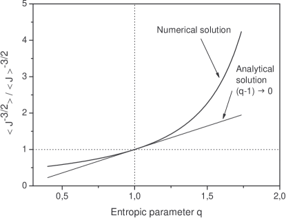
Figure 1: The entropic parameter $q$ is connected to specific moments of the distribution of exchange integrals. This result is valid for any $f(J)$ and shows that the entropic parameter is connected to the physical properties of the system.

An analytical connection between the entropic parameter $q$ and the specific moments of the exchange integral of the inhomogeneous magnetic media can be obtained using the expression for the volume magnetization change in the limit $(q-1)\rightarrow 0$. Comparing the (21) and (28) one gets

$$\frac{\sqrt{\pi}}{2}\,\zeta\left(\frac{3}{2}\right)+2.98\,(q-1)=\frac{\sqrt{\pi}}{2}\,\zeta\left(\frac{3}{2}\right)\frac{\langle J^{-3/2}\,\rangle}{\langle J\rangle^{-3/2}}$$ (37)

or

$$(q-1)=0.78\,\left[\frac{\langle J^{-3/2}\,\rangle}{\langle J\rangle^{-3/2}}-1\right].$$ (38)

The result above is also valid for any $f(J)$ and shows that the entropic parameter is connected to the physical properties of the system [2, 18, 19, 20].

5 Final remarks

Summarizing, in the present work we have shown that the $q$ parameter can be seen as a measurement of the inhomogeneity of a magnetic system. It ratifies previous works [2, 3] in which, inspired in Superstatistics [19], the entropic parameter $q$ was related to the first and second moments of the distribution of magnetic moments of manganites

$$q\,(2-q)^{2}=\frac{\langle\mu^{2}\rangle}{\langle\mu\rangle^{2}}$$ (39)

and was also experimentally verified. Thus, the present work corroborates the idea that changing the usual Boltzmann$-$Gibbs statistics to one that is able to describe power-laws (Tsallis statistics), one can characterize systems that has special features like inhomogeneities; Nonextensivity is therefore a key role to describe complex systems.

References

References

• [1] C. Tsallis. Possible generalization of Boltzman-Gibbs statistics. Journal of Statistical Physics, 52:479, 1988.
• [2] M. S. Reis, V. S. Amaral, R. S. Sarthour, and I. S. Oliveira. Experimental determination of the nonextensive entropic parameter q. Physical Review B, 73:092401, 2006.
• [3] M. S. Reis, V. S. Amaral, R. S. Sarthour, and I. S. Oliveira. Physical meaning and measurement of the entropic parameter q in an inhomogeneous magnetic systems. European Physical Journal B, 50:99, 2006.
• [4] C. Tsallis. Nonextensive Statistics: Theoretical, Experimental and Computational Evidences and Connections. Brazilian Journal of Physics, 29:1, 1999.
• [5] C. Tsallis and E. Brigatti. Nonextensive statistical mechanics: A brief introduction. Continuum Mechanics and Thermodynamics, 16:223, 2004.
• [6] C. Tsallis, M. Gell-Mann, and Y. Sato. Asymptotically scale-invariant occupancy of phase space makes the entropy Sq extensive. Proceedings of the National Academy of Science, 102:15377, 2005.
• [7] C. Tsallis. Entropic nonextensivity: A possible measure of complexity. Chaos Solitons and Fractals, 13:371, 2002.
• [8] F. P. Agostini, D. O. Soares-Pinto, M. A. Moret, C. Oshtoff, and P. G. Pascutti. Generalized Simulated Annealing Applied to Protein Folding Studies. Journal of Computational Chemistry, 27:1142, 2006.
• [9] S. M. D. Queirós, L. G. Moyano, J. de Souza, and C. Tsallis. A nonextensive approach to the dynamics of financial observables. European Physical Journal B, 55:161–167, 2007.
• [10] B. M. Boghosian. Thermodynamic description of the relaxation of two-dimensional turbulence using Tsallis statistics. Physical Review E, 53:4754, 1996.
• [11] C. Beck. Generalized statistical mechanics of cosmic rays. Physica A, 331:173, 2004.
• [12] For a complete and updated list of references, see the web site: tsallis.cat.cbpf.br/biblio.htm.
• [13] M. S. Reis, J. P. Araújo, V. S. Amaral, E. K. Lenzi, and I. S. Oliveira. Magnetic behavior of a nonextensive S-spin system: Possible connections to manganites. Physical Review B, 66:134417, 2002.
• [14] M. S. Reis, V. S. Amaral, J. P. Araújo, and I. S. Oliveira. Magnetic phase diagram for a nonextensive system: Experimental connection with manganites. Physical Review B, 68:014404, 2003.
• [15] A. Moreo, S. Yunoki, and E. Dagotto. The Phase Separation Scenario for Manganese Oxides. Science, 283:2034, 1999.
• [16] E. Dagotto, T. Hotta, and A. Moreo. Colossal magnetoresistant materials: the key role of phase separation. Physics Reports, 344:1, 2001.
• [17] E. Dagotto. Complexity in Strongly Correlated Electronic Systems. Science, 309:257, 2005.
• [18] C. Beck. Dynamical Foundations of Nonextensive Statistical Mechanics. Physical Review Letters, 87:180601, 2001.
• [19] C. Beck and E. G. D. Cohen. Superstatistics. Physica A, 322:267, 2003.
• [20] G. Wilk and Z. Włodarczyk. Interpretation of the Nonextensivity Parameter q in Some Applications of Tsallis Statistics and Lévy Distributions. Physical Review Letters, 84:2770, 2000.
• [21] I. S. Oliveira and V. J. B. de Jesus. Introdução à Física do Estado Sólido, (in Portuguese). Livraria da Física, Brazil, 2005.
• [22] A. P. Guimarães. Magnetism and Magnetic Resonance in Solids. Wiley-Interscience, New York, 1998.
• [23] N. Majlis. The Quantum Theory of Magnetism. World Scientific, Singapore, 2000.
• [24] D. Mattis. The Theory of Magnetism I: Static and Dynamics. Springer, Berlin, 1988.
• [25] A. M. C. Souza and C. Tsallis. Complexity, Metastability and Nonextensivity, chapter Generalizing the Planck distribution. eds. C. Beck, G. Benedek, A. Rapisarda and C. Tsallis. World Scientific, Singapore, 2005.
• [26] M. S. Reis, J. C. C. Freitas, M. T. D. Orlando, E. K. Lenzi, and I. S. Oliveira. Evidences for Tsallis non-extensivity on CMR manganites. Europhysics Letters, 58:42, 2002.