Influence of dissipation on the extraction of quantum states via repeated measurements

Abstract

A quantum system put in interaction with another one that is repeatedly measured is subject to a non-unitary dynamics, through which it is possible to extract subspaces. This key idea has been exploited to propose schemes aimed at the generation of pure quantum states (purification). All such schemes have so far been considered in the ideal situations of isolated systems. In this paper, we analyze the influence of non-negligible interactions with environment during the extraction process, with the scope of investigating the possibility of purifying the state of a system in spite of the sources of dissipation. A general framework is presented and a paradigmatic example consisting of two interacting spins immersed in a bosonic bath is studied. The effectiveness of the purification scheme is discussed in terms of purity for different values of the relevant parameters and in connection with the bath temperature.

I Introduction

During the last decades, enormous progresses have been made in such physical contexts as cavity quantum electrodynamics (CQED) ref:CQED , superconductor-based circuits ref:SCircuits , and trapped ions ref:TrapReview . In connection with the applications in the field of quantum information ref:q_tech , seminal experimental results have been reached, such as the implementations of quantum logical gates ref:NISTCNOT ; ref:BlattCNOT ; ref:NECCNOT and the realizations of quantum teleportation ref:Teleportation . Generation of quantum states is a crucial issue in nano-technologies, because it is the basis of initialization processes with which many experimental protocols begin. Incidentally, it also provides the possibility of observing physical systems behaving according to the predictions of quantum mechanics once a nonclassical state has been created.

Recently, a strategy for the generation of pure quantum states through extraction from arbitrary initial states has been proposed ref:Nakazato_PRL ; ref:Nakazato_PRA . This procedure is based on the idea of putting a quantum system in interaction with another one that is repeatedly measured in order to induce a non-unitary evolution which forces the former system onto a Hilbert subspace. If such a subspace is one-dimensional, the process reduces to the extraction of a pure quantum state. For this reason, this procedure has been addressed as a “purification” ref:q_tech ; ref:Purification . On the basis of this general scheme, many applications have been proposed: it is possible to extract entanglement ref:Nakazato_PRA ; ref:Lidar_PRA-Paternostro , and the initialization of multiple qubits would be useful for quantum computation ref:Nakazato_PRA ; ref:qdot ; extensions of the scheme enable us to establish entanglement between two spatially separated systems via repeated measurements on an entanglement mediator ref:qpfe-separated ; in single trapped ions, the extraction of angular-momentum Schrödinger-cat states has been proposed ref:Militello_PRA04 and the possibility of steering the extraction of pure states through quantum Zeno effect has been predicted ref:Militello_PRA05 . In passing, we mention that the approach here recalled is related to quantum non-demolition measurements ref:general_QND , introduced for gravitational wave detection ref:GravityWaveDetection and exploited in different physical systems for applications in quantum computation and information ref:QND_QuantumInfoQubits and for quantum state generation in general. For instance, in the context of trapped ions, putting the vibrational degrees of freedom in interaction with the electronic degrees of freedom, and repeatedly measuring the atomic state, it is possible to generate Fock states both in one-dimensional ref:TrapOneDim_QND and two-dimensional contexts ref:TrapTwoDim_QND .

Until now, the extraction of pure states through repeated measurements has been considered in ideal situations, that is, the evolution is assumed to be unitary except for the change of state by the measurements. In this paper, we discuss how the predictions change when the system is put in interaction with an environment and, as a consequence, is subject to a non-unitary evolution (even between two successive measurements), which is assumed to be described by a Lindblad-type equation ref:MasterEq . First of all in this paper, we discuss the behavior of a quantum system, whose dynamics is governed by the repeated measurements represented by projection operators on the other system in interaction with the former and by the dissipative environmental interaction with the two quantum systems. A criterion for the extraction of pure states in the presence of dissipation is derived and a quantum system composed of two two-level systems (qubits) immersed in a common bosonic bath is analyzed as a very simple example. The ability or disability of extracting pure states for a one qubit system by this scheme is estimated numerically in terms of the purity of the density operator.

The present paper is organized as follows. In Sec. II, the general aspects of the purification protocol in the presence of interaction with an environment are discussed. In Sec. III, a simple model of two mutually interacting two-level systems immersed in a bosonic bath is analyzed, and the main differences between the ideal situation (in the absence of dissipation) and the more realistic situation here studied (in the presence of dissipation) are singled out. Finally, some conclusive remarks are given in Sec. IV.

II General Framework

II.1 Framework

The scheme of extraction we study in this paper is based on the idea presented in Ref. ref:Nakazato_PRL . Assume that we are interested in preparing a target system, S, into a pure state. To this end, put it in interaction with an ancilla system, X, which is repeatedly measured and found in the same state, say $|{\Phi}\rangle_{\text{X}}$. As a consequence of both the interaction with and the measurements on X, system S is subject to a non-unitary dynamics which forces it in a subspace. If the subspace is one-dimensional, the relevant state is extracted. We underline that if a negative result is obtained measuring system X (i.e., if the ancilla system is found in a state different from the expected one), then the trial can be considered as “failed” and the system has to be reset in order to restart the experiment, or we can just continue the process as a new trial with the initial condition given by the result of the unsuccessful projection.

In the following, we consider this scheme but in the presence of dissipation, in order to examine whether a pure state can still be extracted. To this end, assume now that both S and X are immersed in a bath, so that the dynamics of the whole system S+X between the repeated measurements is governed by the master equation

$$\frac{d\rho_{\text{tot}}}{dt}=\mathcal{L}\rho_{\text{tot}},\qquad\mathcal{L}=\mathcal{H}+\mathcal{D},$$ (1)

where $\rho_{\text{tot}}$ is the density operator of S+X (the trace over the bath degrees of freedom has already been performed). $\mathcal{H}$ is the Hamiltonian superoperator defined by $\mathcal{H}\rho_{\text{tot}}=-i[\hat{H},\rho_{\text{tot}}]$, while $\mathcal{D}$ is the Lindblad-type dissipator ref:MasterEq which takes into account the interaction with the environment, in the Markovian limit. Let $\mathcal{M}(\tau)=e^{\mathcal{L}\tau}$ denote the superoperator describing the dissipative dynamics of S+X and $\mathcal{P}$ the projection superoperator associated with the measurement of the state $|{\Phi}\rangle_{\text{X}}$, i.e.

$$\mathcal{P}\rho_{\text{tot}}=|{\Phi}\rangle_{\text{X}}\langle{\Phi}|\rho_{\text{tot}}|{\Phi}\rangle_{\text{X}}\langle{\Phi}|.$$ (2)

Assuming that the time elapsed between two successive measurements is always $\tau$ and that every of the $N+1$ measurements has confirmed X to be in the state $|{\Phi}\rangle_{\text{X}}$, the initial state $\rho_{\text{tot}}(0)$ is mapped into the final one,

$$\rho_{\text{tot}}(\tau,N)\propto\mathcal{P}\mathcal{M}(\tau)\cdots\mathcal{P}\mathcal{M}(\tau)\mathcal{P}\rho_{\text{tot}}(0)=\mathcal{V}_{\text{tot}}^{N}(\tau)\rho_{\text{tot}}(0),$$ (3)

where

$$\mathcal{V}_{\text{tot}}(\tau)=\mathcal{P}\mathcal{M}(\tau)\mathcal{P},$$ (4)

which, although rigorously speaking acts on Liouville space ref:Rev_Liouville of the whole system S+X, is substantially a superoperator acting on the Liouville space of subsystem S, except for the trivial action on X (i.e. projection on the state $|{\Phi}\rangle_{\text{X}}$). Therefore, it can be rewritten as $\mathcal{V}_{\text{tot}}(\tau)=\mathcal{V}(\tau)\otimes\mathcal{P}$, where $\mathcal{V}(\tau)$ is a superoperator acting only on the Liouville space of S.

If the master equation is given in the Lindblad form ref:MasterEq , the evolution of S+X in interaction with the bath is written down in the Kraus representation ref:KrausRepr as

$$\mathcal{M}(\tau)\rho_{\text{tot}}=\sum_{k=0}^{G}\hat{T}_{k}(\tau)\rho_{\text{tot}}\hat{T}_{k}^{\dagger}(\tau),$$ (5)

where $G+1$ is the number of Kraus operators $\hat{T}_{k}(\tau)$ involved in the decay process. Therefore, the superoperator $\mathcal{V}(\tau)$ that maps the state of S just after a measurement to another after the next measurement reads

$$\mathcal{V}(\tau)\rho=\sum_{k=0}^{G}\hat{V}_{k}(\tau)\rho\hat{V}_{k}^{\dagger}(\tau),$$ (6)

where $\rho$ is the state of S and

$$\hat{V}_{k}(\tau)={}_{\text{X}}\langle{\Phi}|\hat{T}_{k}(\tau)|{\Phi}\rangle_{\text{X}}$$ (7)

is an operator acting on the Hilbert space of S. Note that the state of the whole system S+X after a measurement is factorized like $\rho_{\text{tot}}=\rho\otimes|{\Phi}\rangle_{\text{X}}\langle{\Phi}|$.

The properties of $\mathcal{V}(\tau)$ determine the fate of the state of S, after many repetitions of measurements on X. In fact, assume that $\mathcal{V}(\tau)$ is diagonalizable and consider its spectral decomposition in terms of its eigenprojections ref:MUIR-Halmos :

$$\mathcal{V}(\tau)=\sum_{n}\lambda_{n}\Pi_{n},$$ (8)

where $\Pi_{n}$ is the eigenprojection belonging to the eigenvalue $\lambda_{n}$ and satisfies the ortho-normality and completeness conditions

$$\Pi_{m}\Pi_{n}=\delta_{mn}\Pi_{n},\qquad\sum_{n}\Pi_{n}=1.$$ (9)

The eigenvalues $\lambda_{n}$ are complex-valued in general and ordered in such a way that $|\lambda_{0}|=|\lambda_{1}|=\cdots=|\lambda_{g_{0}}|>|\lambda_{g_{0}+1}|\geq|\lambda_{g_{0}+2}|\geq\cdots{}$. If $\mathcal{V}(\tau)$ is not diagonalizable, the Jordan decomposition applies instead of (8) ref:MUIR-Halmos . Generalization of the following argument to such cases is straightforward. See, for instance, an Appendix of Ref. ref:Nakazato_PRA .

The evaluation of the $N$th power of $\mathcal{V}(\tau)$ shows that, the larger the number $N$ of the repeated measurements is, the more dominant the blocks belonging to the maximum (in modulus) eigenvalues are over the other blocks. That is, for a large enough $N$, the action of $\mathcal{V}^{N}(\tau)$ diminishes the components of the system density operator which do not belong to the generalized eigenspaces corresponding to the maximum (in modulus) eigenvalues. Indeed,

$$\mathcal{V}^{N}(\tau)=\sum_{n}\lambda_{n}^{N}\Pi_{n}\xrightarrow{N\rightarrow\infty}\sum_{n=0}^{g_{0}}\lambda_{n}^{N}\Pi_{n},$$ (10)

which, in the case wherein only one eigenvalue exists whose modulus is maximum (i.e. when $g_{0}=0$), reduces to

$$\mathcal{V}^{N}(\tau)\xrightarrow{N\rightarrow\infty}\lambda_{0}^{N}\Pi_{0}.$$ (11)

Therefore, in such a case, for a large enough (depending on the structure of the spectrum) $N$, the action of $\mathcal{V}^{N}(\tau)$ essentially reduces to the action of $\Pi_{0}$, hence projecting the system in the relevant subspace.

As for the outcome state, it is worth mentioning that, if $\lambda_{0}$ is degenerated, the state of S extracted by $\Pi_{0}$ depends on the initial state of S, $\rho(0)$, since such a final state is substantially proportional to $\Pi_{0}\rho(0)$, which depends on $\rho(0)$ if $\Pi_{0}$ refers to a multi-dimensional space. On the contrary, if $\lambda_{0}$ is not degenerated and $\Pi_{0}$ refers to a one-dimensional subspace, i.e.

$$\Pi_{0}\rho=f_{0}(\rho)\rho_{0}$$ (12)

with $\rho_{0}$ the relevant eigenstate (which is an element of the Liouville space of S) and $f_{0}$ a suitable form on the Liouville space of S, the eigenstate $\rho_{0}$ is extracted irrespectively of the initial condition of the system, provided $\Pi_{0}\rho(0)\not=0$. As a first step, in this paper we shall concentrate on such situations wherein there is a single extracted eigenspace which in addition is one-dimensional.

In an ideal case wherein any sources of dissipation are absent, Eq. (6) reduces to $\mathcal{V}(\tau)\rho=\hat{V}_{0}(\tau)\rho\hat{V}_{0}^{\dagger}(\tau)$ with $\hat{V}_{0}(\tau)={}_{\text{X}}\langle{\Phi}|e^{-i\hat{H}t}|{\Phi}\rangle_{\text{X}}$ ref:Nakazato_PRL , so that, if $\hat{V}_{0}(\tau)$ possesses a nondegenerate and unique maximum (in modulus) eigenvalue, then the final state to be extracted is the pure state $|{u_{0}}\rangle_{\text{S}}\langle{u_{0}}|$, since in this case Eq. (12) is supplemented by $\rho_{0}=|{u_{0}}\rangle_{\text{S}}\langle{u_{0}}|$ and $f_{0}(\rho)={}_{\text{S}}\langle{v_{0}}|\rho|{v_{0}}\rangle_{\text{S}}$ where $|{u_{0}}\rangle$ and $\langle{v_{0}}|$ are the right- and left-eigenvectors of $\hat{V}_{0}(\tau)$ belonging to its largest (in modulus) eigenvalue, respectively. This is the basic idea of the purification scheme based on the repeated measurements, which was first proposed in Ref. ref:Nakazato_PRL and has been analyzed and developed in Refs. ref:Nakazato_PRA ; ref:Lidar_PRA-Paternostro ; ref:qdot ; ref:qpfe-separated ; ref:Militello_PRA04 ; ref:Militello_PRA05 . On the other hand, it is important to stress that in the non-ideal case, even if there is a single and nondegenerate eigenvalue that is maximum in modulus, this does not guarantee that the state $\rho_{0}$ is a pure state and hence there is no warranty that the final extracted state is pure, either. In this sense, our state-extraction scheme may not necessarily be an effective purification scheme. However, we still try to seek a possibility of extracting a pure state even in the presence of dissipation. The examination of such situations wherein we can extract a pure state is the main topic of this paper.

Efficiency — This scheme for extracting quantum states is a conditional one, in the sense that each time system X is measured it has to be found in the same state, denoted by $|{\Phi}\rangle_{\text{X}}$. In Refs. ref:Nakazato_PRL ; ref:Nakazato_PRA ; ref:Lidar_PRA-Paternostro ; ref:qdot ; ref:qpfe-separated ; ref:Militello_PRA04 ; ref:Militello_PRA05 it is proved that the probability of success of the extraction, that is the probability of finding system X in the state $|{\Phi}\rangle_{\text{X}}$ successively $N$ times, is given by the normalization factor of the state extracted by (3), $\mathop{\text{tr}}\nolimits_{\text{S}}\{\mathcal{V}^{N}(\tau)\rho(0)\}=\sum_{n}\lambda_{n}^{N}\mathop{\text{tr}}\nolimits_{\text{S}}\{\Pi_{n}\rho(0)\}$, which behaves asymptotically as $\to\lambda_{0}^{N}\mathop{\text{tr}}\nolimits_{\text{S}}\{\Pi_{0}\rho(0)\}$ as $N\to\infty$ [or $\to\sum_{n\leq g_{0}}\lambda_{n}^{N}\mathop{\text{tr}}\nolimits_{\text{S}}\{\Pi_{n}\rho(0)\}$ in the more general situation, which from now on we shall not mention anymore for the sake of simplicity]. These expressions for the probability of success (still valid in the non-ideal case, provided the projectors $\Pi_{n}$ are the appropriate ones) show that the structure of the spectrum of $\mathcal{V}(\tau)$ plays a crucial role for the efficiency and fastness of the extraction. In particular, on the one hand, the fact that $\lambda_{0}$ has a modulus quite larger than those of the other eigenvalues makes $\mathcal{V}^{N}(\tau)$ quickly approach $\lambda_{0}^{N}\Pi_{0}$, so that a smaller number of measurements is required to well approximate the final result $\Pi_{0}\rho(0)$. On the other hand, the closer to unity the modulus of $\lambda_{0}$ is, the greater the probability of success is, approaching just $\mathop{\text{tr}}\nolimits_{\text{S}}\{\Pi_{0}\rho(0)\}$ (without decaying out completely) for $\lambda_{0}\simeq 1$. On the contrary, for small values of $\lambda_{0}$, the probability quickly approaches zero like $\lambda_{0}^{N}$, which means that if a large number of measurements is required to approach the state $(\mathop{\text{tr}}\nolimits_{\text{S}}\{\Pi_{0}\rho(0)\})^{-1}\Pi_{0}\rho(0)$ the scheme becomes very inefficient. Therefore, the number of measurements necessary to extract the target state would be an important measure of efficiency. It can be roughly estimated by the following argument. The idea is to see how much the relevant part approaching the target state, $\lambda_{0}^{N}\Pi_{0}\rho(0)$, dominates over the rest:

$$p=\frac{\lambda_{0}^{N}\|\Pi_{0}\rho(0)\|}{\sum_{n}|\lambda_{n}|^{N}\|\Pi_{n}\rho(0)\|}\,,$$ (13)

where $\|\cdot\|$ is a certain norm, for instance $\|A\|:={\sqrt{\mathop{\text{tr}}\nolimits_{\text{S}}\{A^{\dagger}A\}}}$. This measure approaches unity in the limit of an infinite number of measurements, $p\to 1$ as $N\to\infty$. Then, we ask how many measurements are necessary for this quantity to exceed a desired value $0<p_{0}<1$. After rewriting (13) as $\lambda_{0}^{N}\|\Pi_{0}\rho(0)\|/(\sum_{n\not=0}|\lambda_{n}|^{N}\|\Pi_{n}\rho(0)\|)=p/(1-p)$, a sufficient condition for $p\geq p_{0}$ is given by

$$\frac{\lambda_{0}^{N}\|\Pi_{0}\rho(0)\|}{(M-1)|\lambda_{1}|^{N}R(\rho(0))}\geq\frac{p_{0}}{1-p_{0}},$$ (14)

where $M$ is the number of eigenvalues or equivalently the dimension of the Liouville space and $R(\rho(0))=\max_{n\not=0}\|\Pi_{n}\rho(0)\|$. The number of measurements necessary to get a better quality than $p_{0}$ is therefore estimated by

$$N\geq\frac{\ln[p_{0}/(1-p_{0})]+\ln(M-1)+\ln\frac{R(\rho(0))}{\|\Pi_{0}\rho(0)\|}}{\ln|\lambda_{0}/\lambda_{1}|}.$$ (15)

It is important to note that this threshold depends on $\rho(0)$, according to the expectation that the larger is the norm of the relevant part in the initial state, $\|\Pi_{0}\rho(0)\|$, the smaller is the number of necessary measurements.

II.2 Searching for Pure Eigenvectors: the Criterion

It is easy to show that a necessary and sufficient condition for a pure state being an eigenvector of the map $\mathcal{V}(\tau)$ is that it is a simultaneous eigenstate of all the operators $\hat{V}_{k}(\tau)$ involved in the relevant map (see Eq. (6)). The proof of this statement proceeds as follows.

$\Longrightarrow$ Obviously, if the state $|{\phi}\rangle_{\text{S}}$ is a common eigenstate of all $\hat{V}_{k}$’s, i.e., $\hat{V}_{k}|{\phi}\rangle_{\text{S}}=\alpha_{k}|{\phi}\rangle_{\text{S}}$ and consequently ${}_{\text{S}}\langle{\phi}|\hat{V}_{k}^{\dagger}={}_{\text{S}}\langle{\phi}|\alpha_{k}^{*}$, then one has

$$\sum_{k=0}^{G}\hat{V}_{k}(\tau)|{\phi}\rangle_{\text{S}}\langle{\phi}|\hat{V}_{k}^{\dagger}(\tau)=\lambda_{\phi}|{\phi}\rangle_{\text{S}}\langle{\phi}|,$$ (16)

where

$$\lambda_{\phi}=\sum_{k}\alpha_{k}^{*}\alpha_{k}\geq 0.$$ (17)

$\Longleftarrow$ Let the pure state $|{\phi}\rangle_{\text{S}}\langle{\phi}|$ be an eigenvector of $\mathcal{V}(\tau)$, then $\sum_{k=0}^{G}\hat{V}_{k}(\tau)|{\phi}\rangle_{\text{S}}\langle{\phi}|\hat{V}_{k}^{\dagger}(\tau)=\lambda_{\phi}|{\phi}\rangle_{\text{S}}\langle{\phi}|$. Consider now the overlap with a quantum state $|{\phi_{\perp}}\rangle_{\text{S}}\langle{\phi_{\perp}}|$ orthogonal to $|{\phi}\rangle_{\text{S}}\langle{\phi}|$:

$$0 =\lambda_{\phi}\,{}_{\text{S}}\langle{\phi_{\perp}}|{\phi}\rangle_{\text{S}}\langle{\phi}|{\phi_{\perp}}\rangle_{\text{S}}$$

$$=\sum_{k=0}^{G}{}_{\text{S}}\langle{\phi_{\perp}}|\hat{V}_{k}(\tau)|{\phi}\rangle_{\text{S}}\langle{\phi}|\hat{V}_{k}^{\dagger}(\tau)|{\phi_{\perp}}\rangle_{\text{S}}$$

$$=\sum_{k=0}^{G}|{}_{\text{S}}\langle{\phi_{\perp}}|\hat{V}_{k}(\tau)|{\phi}\rangle_{\text{S}}|^{2},$$ (18)

from which it follows that ${}_{\text{S}}\langle{\phi_{\perp}}|\hat{V}_{k}(\tau)|{\phi}\rangle_{\text{S}}=0$ for all $k$ and whatever the state $|{\phi_{\perp}}\rangle_{\text{S}}$ is, provided it is orthogonal to $|{\phi}\rangle_{\text{S}}$. In other words, it means that

$$\hat{V}_{k}(\tau)|{\phi}\rangle_{\text{S}}=\alpha_{k}|{\phi}\rangle_{\text{S}},\quad\forall k,$$ (19)

where $\alpha_{k}$ is a suitable complex number. This completes the proof.

II.3 Searching for Pure Eigenvectors: Purity

In those cases in which we are not able to extract an exactly pure state, there is a possibility of extracting “almost pure” states, that is, mixed states very close (in the sense of purity) to the pure states. To look for almost pure states which can be extracted, let us recall a measure of purity of a given state. We show later how the purity of the eigenstate of the linear map $\mathcal{V}(\tau)$ corresponding to the maximum eigenvalue behaves as a function of the parameters of the scheme, i.e. the interval of time $\tau$ and the repeatedly measured state of X, $|{\Phi}\rangle_{\text{X}}$.

The purity of a state is defined as the trace of the square of the relevant (normalized) density operator ref:PurityDef :

$$P(\rho)=\mathop{\text{tr}}\nolimits_{\text{S}}\rho^{2}.$$ (20)

This quantity is upper and lower bounded in accordance with $1/L\leq P(\rho)\leq 1$ with $L$ being the number of levels of the system under scrutiny. Observe that the maximum value [$P(\rho)=1$] corresponds to pure states, while the minimum value [$P(\rho)=1/L$] corresponds to maximally mixed states with maximal von Neumann’s entropy.

II.4 Weak-Damping Case

It is possible to derive a formula for the purity of the extracted state for general systems in the weak-damping regime. Such a formula would be useful for understanding which parameters spoil the purity and convenient for an optimization of the purification.

Let us decompose the relevant map $\mathcal{V}(\tau)$ into two parts,

$$\mathcal{V}(\tau)=\mathcal{V}^{(0)}(\tau)+\delta\mathcal{V}(\tau),$$ (21)

where $\mathcal{V}^{(0)}(\tau)$ is the map in the absence of the environmental perturbation and the rest is treated as a perturbation to it, which is given in the weak-damping regime by

$$\delta\mathcal{V}(\tau)\otimes\mathcal{P}\simeq\int_{0}^{\tau}dt\,\mathcal{P}e^{\mathcal{H}(\tau-t)}\mathcal{D}e^{\mathcal{H}t}\mathcal{P}.$$ (22)

Assuming that $\hat{V}_{0}(\tau)$ is diagonalizable, let $|{u_{n}}\rangle_{\text{S}}$ and ${}_{\text{S}}\langle{v_{n}}|$ denote its right- and left-eigenvectors, respectively, which form a complete ortho-normal set, $\sum_{n}|{u_{n}}\rangle_{\text{S}}\langle{v_{n}}|=\openone_{\text{S}}$ note:degeneracy . (We also normalize the right-eigenvectors as ${}_{\text{S}}\langle{u_{n}}|{u_{n}}\rangle_{\text{S}}=1$.) Then, the right-eigenvectors of the ideal map read

$$\mathcal{V}^{(0)}(\tau)\sigma_{mn}^{(0)}=\lambda_{mn}^{(0)}\sigma_{mn}^{(0)},\quad\sigma_{mn}^{(0)}=|{u_{m}}\rangle_{\text{S}}\langle{u_{n}}|.$$ (23)

These are orthogonal to the left-eigenvectors

$$\tilde{\sigma}_{mn}^{(0)}=|{v_{m}}\rangle_{\text{S}}\langle{v_{n}}|$$ (24)

in the sense

$$(\tilde{\sigma}_{mn}^{(0)},\sigma_{m^{\prime}n^{\prime}}^{(0)})=\delta_{mm^{\prime}}\delta_{nn^{\prime}},\quad(A,B)=\mathop{\text{tr}}\nolimits_{\text{S}}\{A^{\dagger}B\}.$$ (25)

We are interested in a situation where we can purify S in the absence of the environmental perturbation. That is, $\lambda_{00}^{(0)}$ is not degenerated and is the only eigenvalue that is the largest in modulus.

Now, the standard perturbative treatment yields the first-order correction to the right-eigenvector,

$$\delta\sigma_{mn}^{(1)}=-\sum_{m^{\prime}n^{\prime}\neq mn}\sigma_{m^{\prime}n^{\prime}}^{(0)}\frac{(\tilde{\sigma}_{m^{\prime}n^{\prime}}^{(0)},\delta\mathcal{V}(\tau)\sigma_{mn}^{(0)})}{\lambda_{m^{\prime}n^{\prime}}^{(0)}-\lambda_{mn}^{(0)}}\,+\,c\,\sigma_{mn}^{(0)}\,,$$ (26)

where the constant $c$ is set equal to zero by the normalization condition $(\tilde{\sigma}_{mn}^{(0)}+\delta\tilde{\sigma}_{mn}^{(1)},\sigma_{mn}^{(0)}+\delta\sigma_{mn}^{(1)})=1$.

This formula is valid when $\lambda_{mn}^{(0)}$ is not degenerated. We are interested in the state to be extracted, i.e. $\rho_{0}\simeq(\sigma_{00}^{(0)}+\delta\sigma_{00}^{(1)})/(1+\mathop{\text{tr}}\nolimits_{\text{S}}\delta\sigma_{00}^{(1)})$. Since $\lambda_{00}^{(0)}$ has been assumed to be nondegenerated, the formula (26) is valid for $\delta\sigma_{00}^{(1)}$. The purity of $\rho_{0}$ up to this order is therefore given by

$$P(\rho_{0}) \simeq 1-2\,\bigl{(}\mathop{\text{tr}}\nolimits_{\text{S}}\delta\sigma_{00}^{(1)}-{}_{\text{S}}\langle{u_{0}}|\delta\sigma_{00}^{(1)}|{u_{0}}\rangle_{\text{S}}\bigr{)}$$

$$=1-2\sum_{mn\neq 00}{}_{\text{S}}\langle{u_{n}}|\hat{Q}_{0}|{u_{m}}\rangle_{\text{S}}\frac{(\tilde{\sigma}_{mn}^{(0)},\delta\mathcal{V}(\tau)\sigma_{00}^{(0)})}{\lambda_{00}^{(0)}-\lambda_{mn}^{(0)}},$$ (27)

where $\hat{Q}_{0}=\openone_{\text{S}}-|{u_{0}}\rangle_{\text{S}}\langle{u_{0}}|$ is a projection operator.

This is the formula for the purity of the extracted state up to the first order in the decay constants in the weak-damping regime. This shows that, if the state $\sigma_{00}^{(0)}$ to be extracted in the ideal case is an eigenstate of the perturbation, i.e. $\delta\mathcal{V}(\tau)\sigma_{00}^{(0)}\propto\sigma_{00}^{(0)}$, the first-order correction to the purity vanishes and the purification is robust against the environmental perturbation, at least up to this order. This is a weaker version of the criterion discussed in Sec. II.2 and is convenient since the dissipator of a master equation, $\mathcal{D}$, suffices to this criterion without knowing the Kraus operators $\hat{T}_{k}(\tau)$ of the decay process, which may require solving the master equation. Furthermore, this formula would be useful for finding a parameter set that optimizes the purity (minimizes the first-order correction to the purity).

When S is a two-level system, the formula (27) is reduced to

$$P(\rho_{0})\simeq 1-\frac{2}{{}_{\text{S}}\langle{v_{1}}|{v_{1}}\rangle_{\text{S}}}\frac{(\tilde{\sigma}_{11}^{(0)},\delta\mathcal{V}(\tau)\sigma_{00}^{(0)})}{\lambda_{00}^{(0)}-\lambda_{11}^{(0)}}.$$ (28)

III A Simple Model

In this section, we apply the ideas presented above to the case of a simple model. Such a system consists of two mutually-interacting spins immersed in a bosonic bath, one of which is repeatedly measured to purify the other.

III.1 Model

Two-spin system — Consider a system of two interacting spins or pseudo-spins, for instance a couple of identical two-level atoms subjected to a dipolar coupling. Assuming that the matrix elements of the dipole operators are real, and neglecting the counter-rotating terms, one reaches the following Hamiltonian (for details, see Refs. ref:Nakazato_PRA ; ref:TwoSpinsInteracting ):

$$\hat{H}_{\text{tot}}=\sum_{i=\text{S},\text{X}}\frac{\Omega}{2}(1+\hat{\sigma}_{z}^{({i})})+\epsilon(\hat{\sigma}_{+}^{({\text{S}})}\hat{\sigma}_{-}^{({\text{X}})}+\hat{\sigma}_{-}^{({\text{S}})}\hat{\sigma}_{+}^{({\text{X}})})$$ (29)

where $\hat{\sigma}_{z}^{({i})}=|{\uparrow}\rangle_{i}\langle{\uparrow}|-|{\downarrow}\rangle_{i}\langle{\downarrow}|$, $\hat{\sigma}_{+}^{({i})}=|{\uparrow}\rangle_{i}\langle{\downarrow}|=(\hat{\sigma}_{-}^{({i})})^{\dagger}$, $\Omega$ is the Bohr frequency of the two-level system and $\epsilon$ the coupling constant. We have set $\hbar=1$.

The eigenstates of the Hamiltonian are the triplet and singlet two-spin states:

$$|{2}\rangle_{\text{tot}} =|{\uparrow}\rangle_{\text{S}}|{\uparrow}\rangle_{\text{X}},$$ (30a)

$$|{1}\rangle_{\text{tot}} =\frac{1}{\sqrt{2}}\bigl{[}|{\uparrow}\rangle_{\text{S}}|{\downarrow}\rangle_{\text{X}}+|{\downarrow}\rangle_{\text{S}}|{\uparrow}\rangle_{\text{X}}\bigr{]},$$ (30b)

$$|{0}\rangle_{\text{tot}} =|{\downarrow}\rangle_{\text{S}}|{\downarrow}\rangle_{\text{X}},$$ (30c)

$$|{s}\rangle_{\text{tot}} =\frac{1}{\sqrt{2}}\bigl{[}|{\uparrow}\rangle_{\text{S}}|{\downarrow}\rangle_{\text{X}}-|{\downarrow}\rangle_{\text{S}}|{\uparrow}\rangle_{\text{X}}\bigr{]},$$ (30d)

which are common eigenstates of $\hat{\bm{\Sigma}}^{2}$ and $\hat{\Sigma}_{z}$ with $\hat{\bm{\Sigma}}=\frac{1}{2}(\hat{\bm{\sigma}}^{(\text{X})}+\hat{\bm{\sigma}}^{(\text{S})})$, whose eigenvalues are given by $\Sigma(\Sigma+1)$ and $m_{\Sigma}$, respectively. The corresponding eigenenergies are $2\Omega$, $\Omega+\epsilon$, $0$, and $\Omega-\epsilon$, respectively. If we consider the case $\Omega>\epsilon$, then $|{0}\rangle$ is the ground state.

Interaction with a bosonic bath — The interaction with a bosonic bath, whose free Hamiltonian is given by $\hat{H}_{\text{B}}=\int dk\,\omega_{k}\hat{a}_{k}^{\dagger}\hat{a}_{k}$, is modelled through the system-bath interaction Hamiltonian

$$\hat{H}_{\text{I}}=\sum_{i=\text{S},\text{X}}(\hat{B}_{i}+\hat{B}_{i}^{\dagger})(\hat{\sigma}_{+}^{(i)}+\hat{\sigma}_{-}^{(i)}),$$ (31)

where $\hat{B}_{i}=\int dk\,g_{k}(\bm{r}_{i})\hat{a}_{k}$, with $\bm{r}_{i}$ the position of spin $i$ and $g_{k}(\bm{r}_{i})$ the coupling constant between the atom at position $\bm{r}_{i}$ and bath mode $k$. Following the standard derivation ref:ME_Derivation and assuming the spins very close each other in order to have $g_{k}(\bm{r}_{1})\simeq g_{k}(\bm{r}_{2})$, we reach the following master equation in the Schrödinger picture for the density operator $\rho_{\text{tot}}$ of S+X:

$$\frac{d\rho_{\text{tot}}}{dt}={} {-i}[\tilde{H}_{\text{tot}},\rho_{\text{tot}}]$$

$${}+\gamma_{2}(1+n_{-})\mathcal{D}_{21}\rho_{\text{tot}}+\gamma_{1}(1+n_{+})\mathcal{D}_{10}\rho_{\text{tot}}$$

$${}+\gamma_{2}n_{-}\mathcal{D}_{12}\rho_{\text{tot}}+\gamma_{1}n_{+}\mathcal{D}_{01}\rho_{\text{tot}}$$ (32)

with $\mathcal{D}_{ij}\rho_{\text{tot}}=|{j}\rangle_{\text{tot}}\langle{i}|\rho_{\text{tot}}|{i}\rangle_{\text{tot}}\langle{j}|-\frac{1}{2}\{|{i}\rangle_{\text{tot}}\langle{i}|,\rho_{\text{tot}}\}$, $n_{\pm}$ the mean numbers of bosons in the bath modes of frequencies $\Omega\pm\epsilon$, which are the Bohr frequencies between the states involved in the transitions $|{2}\rangle_{\text{tot}}\to|{1}\rangle_{\text{tot}}$ ($\Omega-\epsilon$) and $|{1}\rangle_{\text{tot}}\to|{0}\rangle_{\text{tot}}$ ($\Omega+\epsilon$). $\gamma_{1}$ and $\gamma_{2}$ are the decay rates related to such modes evaluated as the spectral correlation functions of $\hat{B}_{i}+\hat{B}_{i}^{\dagger}$, and are related to $g_{k}$’s by $\gamma_{1}=2\pi\int\,dk\,|g_{k}|^{2}\delta(\omega_{k}-\Omega+\epsilon)$ and $\gamma_{2}=2\pi\int\,dk\,|g_{k}|^{2}\delta(\omega_{k}-\Omega-\epsilon)$. Finally, $\tilde{H}_{\text{tot}}$ is the Lamb-shifted Hamiltonian of S+X.

III.2 Extraction of Pure States under the Influence of a Zero-Temperature Bosonic Bath

Consider now the special case wherein the bath is at zero temperature. The spin labelled with X is repeatedly measured and found in the state $|{\Phi}\rangle_{\text{X}}=\cos\frac{\theta}{2}|{\uparrow}\rangle_{\text{X}}+e^{i\chi}\sin\frac{\theta}{2}|{\downarrow}\rangle_{\text{X}}$, while the other spin, labelled with S, is driven toward a quantum state through its interaction with X. The same situation is discussed in Ref. ref:Nakazato_PRA , in the absence of the environmental coupling, where it is found that the extracted state can be made pure very efficiently, in particular measuring the states $|{\uparrow}\rangle_{\text{X}}$ and $|{\downarrow}\rangle_{\text{X}}$. The evolution of the damped system between two successive measurements is easily evaluated, for instance, following the approach developed in Ref. ref:Nakazato_LANL , and is given by (see Eq. 5)

$$\rho_{\text{tot}}(t)=\sum_{k=0}^{3}\hat{T}_{k}(t)\rho_{\text{tot}}(0)\hat{T}_{k}^{\dagger}(t)$$ (33a)

with 4 Kraus operators,

$$\hat{T}_{0}(t)={} |{0}\rangle_{\text{tot}}\langle{0}|+e^{-\frac{\gamma_{1}}{2}t}e^{-i(\Omega+\epsilon)t}|{1}\rangle_{\text{tot}}\langle{1}|$$

$${}+e^{-\frac{\gamma_{2}}{2}t}e^{-i2\Omega t}|{2}\rangle_{\text{tot}}\langle{2}|+e^{-i(\Omega-\epsilon)t}|{s}\rangle_{\text{tot}}\langle{s}|,$$ (33b)

$$\hat{T}_{1}(t)={} \sqrt{1-e^{-\gamma_{1}t}}|{0}\rangle_{\text{tot}}\langle{1}|,$$ (33c)

$$\hat{T}_{2}(t)={} \sqrt{\frac{\gamma_{2}}{\gamma_{1}-\gamma_{2}}(e^{-\gamma_{2}t}-e^{-\gamma_{1}t})}|{1}\rangle_{\text{tot}}\langle{2}|,$$ (33d)

$$\hat{T}_{3}(t)={} \sqrt{1+\frac{\gamma_{2}e^{-\gamma_{1}t}-\gamma_{1}e^{-\gamma_{2}t}}{\gamma_{1}-\gamma_{2}}}|{0}\rangle_{\text{tot}}\langle{2}|.$$ (33e)

$\hat{T}_{0}(t)$ reduces to the unitary evolution operator in the case $\gamma_{2}=\gamma_{1}=0$, whereas the others, i.e. $\hat{T}_{k}(t)$ for $k\geq 1$, vanish.

Now measure system X repeatedly every after $\tau$ during the dissipative dynamics (33). According to (19), in order for the S state $|{\phi}\rangle_{\text{S}}\langle{\phi}|$, with $|{\phi}\rangle_{\text{S}}=\cos\frac{\eta}{2}|{\uparrow}\rangle_{\text{S}}+e^{i\xi}\sin\frac{\eta}{2}|{\downarrow}\rangle_{\text{S}}$, be a pure eigenstate of the contracted map $\mathcal{V}(\tau)$, it should satisfy

$$s_{k}(\tau)\equiv{}_{\text{S}}\langle{\phi_{\perp}}|{}_{\text{X}}\langle{\Phi}|\hat{T}_{k}(t)|{\Phi}\rangle_{\text{X}}|{\phi}\rangle_{\text{S}}=0,\quad k=0,1,2,3$$ (34)

with $|{\phi_{\perp}}\rangle_{\text{S}}=\sin\frac{\eta}{2}|{\uparrow}\rangle_{\text{S}}-e^{i\xi}\cos\frac{\eta}{2}|{\downarrow}\rangle_{\text{S}}$. Indeed, it is equivalent to look for the eigenstates of the contracted operators $\hat{V}_{k}(\tau)$ defined in (7). It is straightforward to find that

$$\begin{cases}\vskip 6.0pt plus 2.0pt minus 2.0pts_{1}(\tau)\propto\sin\frac{\theta}{2}\cos\frac{\eta}{2}\left(e^{i\xi}\cos\frac{\theta}{2}\sin\frac{\eta}{2}+e^{i\chi}\sin\frac{\theta}{2}\cos\frac{\eta}{2}\right),\\ \vskip 6.0pt plus 2.0pt minus 2.0pts_{2}(\tau)\propto\cos\frac{\theta}{2}\cos\frac{\eta}{2}\left(e^{-i\chi}\sin\frac{\theta}{2}\sin\frac{\eta}{2}-e^{-i\xi}\cos\frac{\theta}{2}\cos\frac{\eta}{2}\right),\\ s_{3}(\tau)\propto\sin\frac{\theta}{2}\cos\frac{\theta}{2}\sin\frac{\eta}{2}\cos\frac{\eta}{2},\end{cases}$$ (35)

where the proportionality factors are the nonvanishing coefficients in (33c)–(33e). From these expressions, it follows that $s_{1}(\tau)=s_{2}(\tau)=s_{3}(\tau)=0$ is accomplished only for $\cos\frac{\eta}{2}=0$. This condition is necessary and sufficient to make $s_{k}$’s vanish for $k=1,2,3$. In order to make $s_{0}(t)$ vanish too, it is necessary to have $\sin\frac{\theta}{2}=0$ or $\cos\frac{\theta}{2}=0$. In fact, the condition $\cos\frac{\eta}{2}=0$ means $|{\phi}\rangle_{\text{S}}=|{\downarrow}\rangle_{\text{S}}$, and evaluating $s_{0}(t)$ in such a special situation provides

$$s_{0}(\tau) ={}_{\text{S}}\langle{\uparrow}|{}_{\text{X}}\langle{\Phi}|\hat{T}_{0}(\tau)|{\Phi}\rangle_{\text{X}}|{\downarrow}\rangle_{\text{S}}$$

$$=-\frac{e^{-i\chi}e^{-i(\Omega-\epsilon)\tau}}{\sqrt{2}}\sin\frac{\theta}{2}\cos\frac{\theta}{2}(1-e^{-\frac{\gamma_{1}}{2}\tau}e^{-i2\epsilon\tau}),$$ (36)

which, for $\tau\not=0$, vanishes only if $\sin\frac{\theta}{2}=0$ or $\cos\frac{\theta}{2}=0$.

This analysis shows that in some special cases, that is, when the state of X is repeatedly measured and found in $|{\Phi}\rangle_{\text{X}}=|{\uparrow}\rangle_{\text{X}}$ ($\sin\frac{\theta}{2}=0$) or $|{\Phi}\rangle_{\text{X}}=|{\downarrow}\rangle_{\text{X}}$ ($\cos\frac{\theta}{2}=0$), the contracted linear map $\mathcal{V}(\tau)$ has the S state $|{\downarrow}\rangle_{\text{S}}\langle{\downarrow}|$ as a pure eigenstate. To reach the final conclusion about the possibility of extracting such a pure state, one needs to know whether the corresponding eigenvalue is the maximum (in modulus) in the spectrum of the map. We shall therefore diagonalize the contracted map in the two cases, $\sin\frac{\theta}{2}=0$ and $\cos\frac{\theta}{2}=0$.

Representing the density operator of S as a four-dimensional vector, $\rho=(\rho_{\uparrow\uparrow},\rho_{\downarrow\downarrow},\rho_{\uparrow\downarrow},\rho_{\downarrow\uparrow})=({}_{\text{S}}\langle{\uparrow}|\rho|{\uparrow}\rangle_{\text{S}},{}_{\text{S}}\langle{\downarrow}|\rho|{\downarrow}\rangle_{\text{S}},{}_{\text{S}}\langle{\uparrow}|\rho|{\downarrow}\rangle_{\text{S}},{}_{\text{S}}\langle{\downarrow}|\rho|{\uparrow}\rangle_{\text{S}})$, the contracted linear map $\mathcal{V}(\tau)$ is substantially represented by a $4\times 4$ matrix.

Repeatedly measuring $|{\downarrow}\rangle_{\text{X}}$ ($\theta=\pi$) — In the case where the X state $|{\downarrow}\rangle_{\text{X}}$ is repeatedly measured, the corresponding linear map $\mathcal{V}(\tau)=\mathcal{V}_{\downarrow}(\tau)$ is represented by the following matrix:

$$\mathcal{V}_{\downarrow}(\tau)=\begin{pmatrix}|f_{\downarrow}(\tau)|^{2}&0&0&0\\ \frac{1}{2}(1-e^{-\gamma_{1}\tau})&1&0&0\\ 0&0&f_{\downarrow}(\tau)&0\\ 0&0&0&f_{\downarrow}^{*}(\tau)\end{pmatrix},$$ (37)

with $f_{\downarrow}(\tau)=\frac{1}{2}e^{-i(\Omega-\epsilon)\tau}(1+e^{-\frac{\gamma_{1}}{2}\tau}e^{-i2\epsilon\tau})$. The eigenvalues of this matrix are

$$\lambda_{0}=1,\quad\lambda_{1}=\lambda_{2}^{*}=f_{\downarrow}(\tau),\quad\lambda_{3}=|f_{\downarrow}(\tau)|^{2}.$$ (38)

The right-eigenvector corresponding to the maximum eigenvalue $\lambda_{0}=1$ is the pure state $\rho_{0}=|{\downarrow}\rangle_{\text{S}}\langle{\downarrow}|$. The larger the time $\tau$ is, the smaller the other three eigenvalues of the map are and the faster the extraction of $\rho_{0}=|{\downarrow}\rangle_{\text{S}}\langle{\downarrow}|$ is, in the sense that it requires a smaller number of steps.

Repeatedly measuring $|{\uparrow}\rangle_{\text{X}}$ ($\theta=0$) — In the case wherein the X state $|{\uparrow}\rangle_{\text{X}}$ is repeatedly measured, the map $\mathcal{V}(\tau)$ reduces to

$$\mathcal{V}_{\uparrow}(\tau)=\begin{pmatrix}e^{-\gamma_{2}\tau}&0&0&0\\ \frac{\gamma_{2}(e^{-\gamma_{2}\tau}-e^{-\gamma_{1}\tau})}{2(\gamma_{1}-\gamma_{2})}&|f_{\uparrow}(\tau)|^{2}&0&0\\ 0&0&e^{-\frac{\gamma_{2}}{2}\tau}f_{\uparrow}(\tau)&0\\ 0&0&0&e^{-\frac{\gamma_{2}}{2}\tau}f_{\uparrow}^{*}(\tau)\end{pmatrix}$$ (39)

with $f_{\uparrow}(\tau)=\frac{1}{2}e^{-i(\Omega+\epsilon)\tau}(1+e^{-\frac{\gamma_{1}}{2}\tau}e^{i2\epsilon\tau})$. This matrix is easily and exactly diagonalized as long as $e^{-\gamma_{2}\tau}\neq|f_{\uparrow}(\tau)|^{2}$. There are two cases in the ordering of its eigenvalues. Case I: if $e^{-\frac{\gamma_{2}}{2}\tau}<|f_{\uparrow}(\tau)|$,

$$\lambda_{0}=|f_{\uparrow}(\tau)|^{2},\quad\lambda_{1}=\lambda_{2}^{*}=e^{-\frac{\gamma_{2}}{2}\tau}f_{\uparrow}(\tau),\quad\lambda_{3}=e^{-\gamma_{2}\tau}.$$ (40)

Case II: if $e^{-\frac{\gamma_{2}}{2}\tau}>|f_{\uparrow}(\tau)|$,

$$\lambda_{0}=e^{-\gamma_{2}\tau},\quad\lambda_{1}=\lambda_{2}^{*}=e^{-\frac{\gamma_{2}}{2}\tau}f_{\uparrow}(\tau),\quad\lambda_{3}=|f_{\uparrow}(\tau)|^{2}.$$ (41)

In case I (which surely occurs in the strong-damping regime $\gamma_{2}\tau\rightarrow\infty$), a pure state $\rho^{\text{(I)}}=|{\downarrow}\rangle_{\text{S}}\langle{\downarrow}|$ is extracted, while in case II, a mixed state is extracted,

$$\rho^{\text{(II)}}=p_{\uparrow\uparrow}|{\uparrow}\rangle_{\text{S}}\langle{\uparrow}|+p_{\downarrow\downarrow}|{\downarrow}\rangle_{\text{S}}\langle{\downarrow}|$$ (42a)

with

$$p_{\uparrow\uparrow}=\frac{1}{1+\alpha},\qquad p_{\downarrow\downarrow}=1-p_{\uparrow\uparrow}=\frac{\alpha}{1+\alpha},$$ (42b)

$$\alpha=\frac{\gamma_{2}(e^{-\gamma_{2}\tau}-e^{-\gamma_{1}\tau})}{2(\gamma_{1}-\gamma_{2})(e^{-\gamma_{2}\tau}-|f_{\uparrow}(\tau)|^{2})}.$$ (42c)

The latter is not in contradiction with the previous statement that one has a pure eigenstate for $\sin\frac{\theta}{2}=0$. Indeed, the state $|{\downarrow}\rangle_{\text{S}}\langle{\downarrow}|$ is still an eigenstate of the map, but it does not correspond to the maximum eigenvalue anymore, and then it is not the state to be extracted.

The purity of the state $\rho^{\text{(II)}}$ in (42) is given by

$$P(\rho^{\text{(II)}})=p_{\uparrow\uparrow}^{2}+p_{\downarrow\downarrow}^{2}=\frac{1+\alpha^{2}}{(1+\alpha)^{2}}.$$ (43)

In the weak-damping case $\gamma_{1}\tau,\gamma_{2}\tau\ll 1$ (and assuming $\sin\epsilon\tau\not=0$ for simplicity), one has $\alpha\simeq\frac{\gamma_{2}\tau}{2\sin^{2}\!\epsilon\tau}$ up to the first order in $\gamma_{1}\tau$ and $\gamma_{2}\tau$, and hence

$$P(\rho^{\text{(II)}})\simeq 1-2\alpha\simeq 1-\frac{\gamma_{2}\tau}{\sin^{2}\!\epsilon\tau}.$$ (44)

This formula, that alternatively can be directly derived using (28), shows that in the weak-damping regime (i) the purity is linearly affected by $\gamma_{2}$, while (ii) it is not influenced by $\gamma_{1}$. Furthermore, (iii) the purity is optimized by taking a nontrivial time interval $\tau\simeq 0.37\pi/\epsilon$.

It is worth noting that in the weak damping limit we cannot extract a pure state, while in the strong damping limit a pure state can be obtained, which is the opposite one would expect. To understand this fact, consider first of all that S$+$X has two stable states, $|{0}\rangle_{\text{tot}}\langle{0}|$ and $|{s}\rangle_{\text{tot}}\langle{s}|$ according to (33), and second that in the strongly dissipative case the system has time to relax onto the equilibrium state which is a mixture of the two stable states, whose statistical weights are determined by the initial condition. Then, repeatedly measuring the state $|{\uparrow}\rangle_{\text{X}}$ cuts the population of $|{0}\rangle_{\text{tot}}$ in the mixture and leaves only ${}_{\text{X}}\langle{\uparrow}|{s}\rangle_{\text{tot}}\langle{s}|{\uparrow}\rangle_{\text{X}}\propto|{\downarrow}\rangle_{\text{S}}\langle{\downarrow}|$.

The case $e^{-\frac{\gamma_{2}}{2}\tau}=|f_{\uparrow}(\tau)|$ corresponds to a degenerate case and hence, as clarified in Sec. II, is not in the scope of this paper since it does not permit the extraction of a precise state irrespectively of the initial state of the system.

Notice that the general case corresponding to measuring a generic state $|{\Phi}\rangle_{\text{X}}$ can be discussed in the weak damping limit through the perturbation analysis.

III.3 At Finite Temperature

The analysis on the model has so far been focused on the zero-temperature case and showed that the only pure state that can be extracted at the zero temperature is $|{\downarrow}\rangle_{\text{S}}$ when the state of X is repeatedly measured and found in $|{\uparrow}\rangle_{\text{X}}$ or $|{\downarrow}\rangle_{\text{X}}$. The question of what happens in the case of non-zero temperature naturally arises. To answer this question, we resort to numerical calculations.

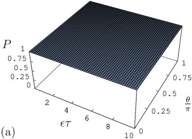
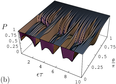
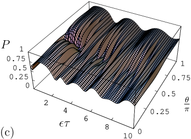
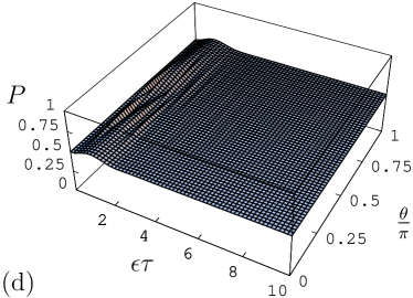
Figure 1: The purity of the extracted state vs the parameters $\epsilon\tau$ and $\theta/\pi$ ($\chi=0$ for all cases), in different situations: (a) in the ideal case, i.e. in the absence of interaction with the bath, and in the presence of interaction with the bath with (b) ${k_{\text{B}}T}/{\hbar\Omega}=0.01$, (c) ${k_{\text{B}}T}/{\hbar\Omega}=1$, and (d) ${k_{\text{B}}T}/{\hbar\Omega}=10$. In all cases, ratios between salient physical quantities are fixed as ${\Omega}/{\epsilon}=10$, ${\gamma_{2}}/{\epsilon}=0.1$, ${\gamma_{1}}/{\gamma_{2}}=0.95$.

The linear map ${\mathcal{V}}(\tau)$ depends on $\tau$, the measured state $|{\Phi}\rangle_{\text{X}}$ (which is individualized in the Bloch-sphere by the polar and azimuthal angles, $\theta$ and $\chi$, respectively), and in general the temperature of the environment, $T$. Given the map, the eigenvector associated with the maximum eigenvalue, and its purity are functions of all such quantities ($\tau$, $\theta$, $\chi$ and $T$).

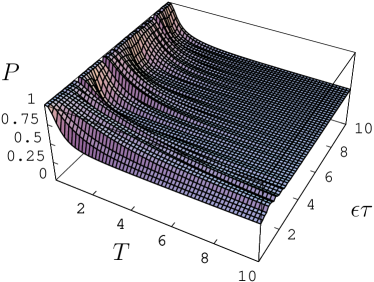
Figure 2: The purity of the extracted state as a function of the temperature $T$ (in units of $\hbar\Omega/k_{\text{B}}$) and $\epsilon\tau$. The other parameters are: $\theta=3\pi/4$, $\chi=0$, ${\Omega}/{\epsilon}=10$, ${\gamma_{2}}/{\epsilon}=0.1$, ${\gamma_{1}}/{\gamma_{2}}=0.95$.

In Fig. 1, the purity of the state to be extracted is shown as a function of the parameters $\tau$ and $\theta$ with $\chi=0$ being fixed, in four different situations concerning the bath. For the numerical calculations, we have set ${\Omega}/{\epsilon}=10$, ${\gamma_{2}}/{\epsilon}=0.1$, and ${\gamma_{1}}/{\gamma_{2}}=0.95$.

In Fig. 1(a), the purity of the state to be extracted in the ideal situation is plotted, that is, in the absence of interaction with the bath. According to the discussion in Sec. II, the purity in such a case is expected to be equal to $1$ whatever the parameters $\tau$, $\theta$ and $\chi$ are. In the other three figures, the behavior of purity in the presence of interaction with the bath at different temperatures is shown. Figure 1(b) refers to the case of very low temperature, effectively zero, and shows that in some regions of the parameter space, there is a possibility of extracting pure or almost pure states. This is not in contradiction with the analysis in Sec. III.2, where it has been found that a pure state can be extracted only for $\theta=0,\pi$. This result refers to an exactly pure eigenstate, while the numerical calculations here reported show the value of purity, which can be very close to unity although not exactly $1$.

In Fig. 1(c), one can see that in practice there is no region in the parameter space corresponding to pure states: the purity is visibly smaller than unity everywhere. Finally, in Fig. 1(d), we see that at a higher temperature ($k_{\text{B}}T=10\hbar\Omega$, with $k_{\text{B}}$ the Boltzmann constant), the purity of the state to be extracted is equal to the minimum value for the two-level system, $\frac{1}{2}$, almost everywhere, that is, irrespectively of the values of parameters $\tau$ and $\theta$.

In Fig. 2, the purity is plotted as a function of the temperature $T$ and of the time interval $\tau$ between successive measurements, when a fixed state of system X characterized by $\theta=3\pi/4$ and $\chi=0$ is repeatedly measured. It is well visible that the more the temperature increases, the more the purity of the extracted state approaches the minimum value, that is, $\frac{1}{2}$.

All these results express in a clear way that the interaction with an environment deteriorates the reliability of the purification scheme based on repeated measurements, although at the zero temperature pure states can still be extracted.

III.4 Efficiency

In a realistic situation, the probability of extracting the target state as well as the number of measurements one has to perform are important factors to consider. According to the discussion at the end of Sec. II.1, the probability of success is asymptotically given by $\lambda_{0}^{N}\mathop{\text{tr}}\nolimits_{\text{S}}\{\Pi_{0}\rho(0)\}$. Therefore, except for those situations wherein the maximum eigenvalue (in modulus) is unity, the most relevant condition to get a good efficiency is that the number of required measurements is very low, which implies $|\lambda_{1}/\lambda_{0}|\ll 1$, or, better, that the denominator in the threshold given in (15) is high, i.e. $\ln\left|\lambda_{0}/\lambda_{1}\right|\gg 1$. Therefore, the peaks of $\ln\left|\lambda_{0}/\lambda_{1}\right|$ correspond to the maxima of the efficiency (i.e., the minima of the required number of measurements). To better fix the idea, if we ask that the target state is obtained with a precision $p_{0}=0.99$, since we have $\ln(4-1)+\ln[p_{0}/(1-p_{0})]\approx 5.7$ we find that, in correspondence to those peaks wherein $\ln\left|\lambda_{0}/\lambda_{1}\right|\sim 4$, the process requires one or two measurements when the system starts with an initial condition satisfying $\|\Pi_{0}\rho(0)\|\sim R(\rho(0))$, which for instance is usually the case for the maximally mixed state.

In Fig. 3(a), we consider the ideal case, while in Figs. 3(b)–3(d), we refer to non-ideal situations at zero, intermediate, and high temperature. The plots clearly show that the interaction with a nonzero temperature environment negatively affects the efficiency, lowering the peaks and extending the valleys. Nevertheless, at zero temperature, various peaks are still present, and in fact, at zero temperature, the degradation with respect to the ideal case is not so dramatic.

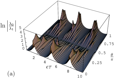
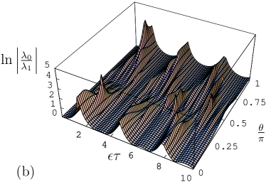
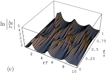
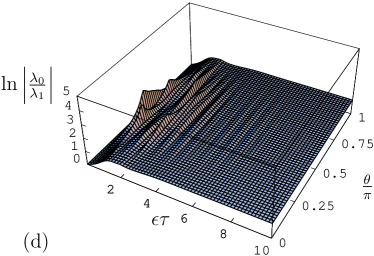
Figure 3: The quantity $\ln\left|\lambda_{0}/\lambda_{1}\right|$ vs the parameters $\epsilon\tau$ and $\theta/\pi$ ($\chi=0$ for all cases), in different situations: (a) in the ideal case, i.e. in the absence of interaction with the bath, and in the presence of interaction with the bath with (b) ${k_{\text{B}}T}/{\hbar\Omega}=0.01$, (c) ${k_{\text{B}}T}/{\hbar\Omega}=1$, and (d) ${k_{\text{B}}T}/{\hbar\Omega}=10$. In all cases, ratios between salient physical quantities are fixed as ${\Omega}/{\epsilon}=10$, ${\gamma_{2}}/{\epsilon}=0.1$, ${\gamma_{1}}/{\gamma_{2}}=0.95$.

IV Summary

Let us summarize the results reported in this paper. Putting a system in interaction with a repeatedly measured one forces the former system onto a subspace, hence realizing, under suitable conditions, the extraction of pure states. In a more realistic situation, the two systems are interacting with their environment too, and therefore are subjected to dissipation. Such an interaction practically reduces the chance to extract pure states.

From the mathematical point of view, the main difference between the two situations is represented by the fact that in the ideal case one extracts eigenvectors of a map onto a Hilbert space, whereas in the non-ideal case one extracts eigenvectors of a map onto a Liouville space. We have explored the general framework and studied a very simple physical system (two spins interacting with a bosonic bath) in order to bring to light fundamental features of repeated-measurement based extraction processes in the presence of dissipation. In Sec. III.2, we have shown that a mixed state is extracted instead of a pure state. Actually, this is what generally happens, especially at high temperatures. Nevertheless, with a zero-temperature bath, it is still possible to extract pure and almost pure states (see Fig. 1(b)) with still fairly good efficiency.

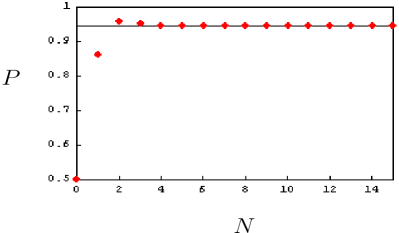
Figure 4: The purity of the state of system S as a function of the number of measurements on X. The initial state is $\rho(0)=0.5|{\uparrow}\rangle_{\text{S}}\langle{\uparrow}|+0.5|{\downarrow}\rangle_{\text{S}}\langle{\downarrow}|$ and its purity is $0.5$. Observe that the purity reaches the maximum value at $N=2$ and then decays to an asymptotic value. Here, the parameters are $\chi=0$, $\theta=2.25$, and $\epsilon\tau=7.82$, and we have set $k_{\text{B}}T/\hbar\Omega=10^{-3}$, ${\Omega}/{\epsilon}=10$, ${\gamma_{2}}/{\epsilon}=0.1$, ${\gamma_{1}}/{\gamma_{2}}=0.95$.

Indeed, the efficiency, though negatively affected by the environment, is still good at zero temperature.

Overall, we have considered the case wherein a very large number of measurements (evaluating the mathematical limit for an infinite number of measurements) is performed on the ancilla system, as clearly expressed by (10) and (11). We conclude this paper expecting that in some cases a reduction of the number of measurements performed on the ancilla system entails an increase of the purity of the output state. See, for example, Fig. 4, wherein we have plotted the purity of the resulting quantum state as a function of the number of measurements performed on the ancilla system, starting from the maximally mixed initial state, with a particular parameter set. It is well visible that the purity, starting from its minimum value ($\frac{1}{2}$), increases at the second measurement, and then decreases down to its asymptotic value. Therefore, in such a case, the highest value of purity is obtained for a smaller number of measurements ($N=2$). We will discuss this aspect of our scheme in the next future.

References

- (1) J. M. Raimond, M. Brune, and S. Haroche, Rev. Mod. Phys. 73, 565 (2001).
- (2) Y. Makhlin, G. Schön, and A. Shnirman, Rev. Mod. Phys. 73, 357 (2001).
- (3) For reviews on trapped ions, see: P. E. Toschek, in New Trends in Atomic Physics, edited by G. Grynberg and R. Stora, Les Houches Summer School Proceedings, Session XXXVIII (North-Holland, Amsterdam, 1984), Vol. 1, p. 381; D. J. Wineland, C. Monroe, W. M. Itano, D. Leibfried, B. E. King, and D. M. Meekhof, J. Res. Natl. Inst. Stand. Technol. 103, 259 (1998); W. Vogel and S. Wallentowitz, in Coherence and Statistics of Photons and Atoms, edited by J. Peřina (Wiley, New York, 2001), p. 333; D. Leibfried, R. Blatt, C. Monroe, and D. Wineland, Rev. Mod. Phys. 75, 281 (2003); F. G. Major, V. N. Gheorghe, and G. Werth, Charged Particle Traps (Springer-Verlag, Berlin, 2004).
- (4) For reviews on quantum information, see: The Physics of Quantum Information, edited by D. Bouwmeester, A. Zeilinger, and A. Ekert (Springer-Verlag, Berlin, 2000); M. A. Nielsen and I. L. Chuang, Quantum Computation and Quantum Information (Cambridge University Press, Cambridge, 2000); C. H. Bennett and D. P. DiVincenzo, Nature (London) 404, 247 (2000); A. Galindo and M. A. Martín-Delgado, Rev. Mod. Phys. 74, 347 (2002).
- (5) B. DeMarco, A. Ben-Kish, D. Leibfried, V. Meyer, M. Rowe, B. M. Jelenković, W. M. Itano, J. Britton, C. Langer, T. Rosenband, and D. J. Wineland, Phys. Rev. Lett. 89, 267901 (2002).
- (6) F. Schmidt-Kaler, H. Häffner, M. Riebe, S. Gulde, G. P. T. Lancaster, T. Deuschle, C. Becher, C. F. Roos, J. Eschner, and R. Blatt, Nature (London) 422, 408 (2003); F. Schmidt-Kaler, H. Häffner, S. Gulde, M. Riebe, G. P. T. Lancaster, T. Deuschle, C. Becher, W. Hänsel, J. Eschner, C. F. Roos, and R. Blatt, Appl. Phys. B 77, 789 (2003).
- (7) T. Yamamoto, Yu. A. Pashkin, O. Astafiev, Y. Nakamura, and J. S. Tsai, Nature (London) 425, 941 (2003).
- (8) M. Riebe, H. Häffner, C. F. Roos, W. Hänsel, J. Benhelm, G. P. T. Lancaster, T. W. Körber, C. Becher, F. Schmidt-Kaler, D. F. V. James, and R. Blatt, Nature (London) 429, 734 (2004); M. D. Barrett, J. Chiaverini, T. Schaetz, J. Britton, W. M. Itano, J. D. Jost, E. Knill, C. Langer, D. Leibfried, R. Ozeri, and D. J. Wineland, ibid. 429, 737 (2004).
- (9) H. Nakazato, T. Takazawa, and K. Yuasa, Phys. Rev. Lett. 90, 060401 (2003).
- (10) H. Nakazato, M. Unoki, and K. Yuasa, Phys. Rev. A 70, 012303 (2004).
- (11) C. H. Bennett, G. Brassard, S. Popescu, B. Schumacher, J. A. Smolin, and W. K. Wootters, Phys. Rev. Lett. 76, 722 (1996); 78, 2031(E) (1997); C. H. Bennett, D. P. DiVincenzo, J. A. Smolin, and W. K. Wootters, Phys. Rev. A 54, 3824 (1996); J. I. Cirac, A. K. Ekert, and C. Macchiavello, Phys. Rev. Lett. 82, 4344 (1999).
- (12) L.-A. Wu, D. A. Lidar, and S. Schneider, Phys. Rev. A 70, 032322 (2004); M. Paternostro and M. S. Kim, New J. Phys. 7, 43 (2005).
- (13) K. Yoh, K. Yuasa, and H. Nakazato, Physica E 29, 674 (2005); K. Yuasa, K. Okano, H. Nakazato, S. Kashiwada, and K. Yoh, AIP Conf. Proc. 893, 1109 (2007).
- (14) G. Compagno, A. Messina, H. Nakazato, A. Napoli, M. Unoki, and K. Yuasa, Phys. Rev. A 70, 052316 (2004); K. Yuasa and H. Nakazato, Prog. Theor. Phys. 114, 523 (2005); J. Phys. A 40, 297 (2007).
- (15) B. Militello and A. Messina, Phys. Rev. A 70, 033408 (2004); Acta Phys. Hung. B 20, 253 (2004).
- (16) B. Militello, H. Nakazato, and A. Messina, Phys. Rev. A 71, 032102 (2005); B. Militello, A. Messina, and H. Nakazato, Opt. Spectrosc. 99, 438 (2005).
- (17) V. B. Braginsky and F. Ya. Khalili, Quantum Measurement (Cambridge University Press, Cambridge, 1992); D. F. Walls and G. J. Milburn, Quantum Optics (Springer, Berlin, 1994).
- (18) P. Grangier, J. A. Levenson, and J.-P. Poizat, Nature (London) 396, 537 (1998).
- (19) L. Mišta, Jr. and R. Filip, Phys. Rev. A 72, 034307 (2005); T. C. Ralph, S. D. Bartlett, J. L. O’Brien, G. J. Pryde, and H. M. Wiseman, ibid. 73, 012113 (2006); J. H. Shapiro and R. S. Bondurant, ibid. 73, 022301 (2006).
- (20) R. L. de Matos Filho and W. Vogel, Phys. Rev. Lett. 76, 4520 (1996); L. Davidovich, M. Orszag, and N. Zagury, Phys. Rev. A 54, 5118 (1996).
- (21) K. Wang, S. Maniscalco, A. Napoli, and A. Messina, Phys. Rev. A 63, 043419 (2001).
- (22) V. Gorini, A. Kossakowski, and E. C. G. Sudarshan, J. Math. Phys. 17, 821 (1976); G. Lindblad, Commun. Math. Phys. 48, 119 (1976).
- (23) S. Mukamel, Principles of Nonlinear Optical Spectroscopy (Oxford University Press, Oxford, 1995).
- (24) E. C. G. Sudarshan, P. M. Mathews, and J. Rau, Phys. Rev. 121, 920 (1961); K. Kraus, Ann. Phys. (N.Y.) 64, 311 (1971); States, Effects, and Operations (Springer-Verlag, Berlin, 1983).
- (25) T. Muir, A Treatise on the Theory of Determinants (Dover Publications, New York, 2003); P. R. Halmos, Finite-Dimensional Vector Spaces (Springer-Verlag, New York, 1974).
- (26) U. Fano, Rev. Mod. Phys. 29, 74 (1957).
- (27) In this subsection, degenerate eigenvalues, if any, are “unfolded,” e.g., a three-fold degenerated eigenvalue is given three different subscripts to distinguish the three linearly independent vectors belonging to it.
- (28) S. Nicolosi, A. Napoli, A. Messina, and F. Petruccione, Phys. Rev. A 70, 022511 (2004).
- (29) H.-P. Breuer and F. Petruccione, The Theory of Open Quantum Systems (Oxford University Press, Oxford, 2002); C. W. Gardiner and P. Zoller, Quantum Noise, 3rd ed. (Springer, Berlin, 2004); P. Facchi, S. Tasaki, S. Pascazio, H. Nakazato, A. Tokuse, and D. A. Lidar, Phys. Rev. A 71, 022302 (2005).
- (30) H. Nakazato, Y. Hida, K. Yuasa, B. Militello, A. Napoli, and A. Messina, Phys. Rev. A 74, 062113 (2006).
- (31) E. M. Corson, Perturbation Methods in the Quantum Mechanics of -Electron Systems (Blackie and Son, London, 1953).