Analysis on Heavy Quarkonia Transitions with Pion Emission in Terms of the QCD Multipole Expansion and Determination of Mass Spectra of Hybrids

I Introduction

In both the quark model and QCD which governs strong interaction, there is no any fundamental principle to prohibit existence of exotic hadron states such as glueball, hybrid and multi-quark states. In fact, to eventually understand the low energy behavior of QCD, one needs to find out such states. However, the recent research indicates that they may mix with the ordinary hadrons especially the quarkonia. Thus they evade direct detection so far, even though many new resonances which have peculiar characteristics, have continuously been reported by various experimental collaborations. Theorists have proposed them to be pure gluonic (glueball), quark-gluon (hybrid), and/or multi-quark (tetraqurk or pentaquark) structures which are different from the regular valence quark structure of $q\bar{q}$ for meson and $qqq$ for baryon. Since the quark model and QCD theory advocate their existence, at least do not repel them, one should find them in experiments. However, even with many candidates of the exotic states, so far none of them have been confirmed yet. Moreover, the possible mixing of such exotic states with the regular mesons or baryons contaminates the situation and would make a clear identification difficult, even though not impossible. From the theoretic aspect, one may try to help to clean the mist and find an effective way to do the job.

The transition of heavy quarkonia such as $\psi(ns)$ and $\Upsilon(ns)$ to lower states $\psi(ms)$ and $\Upsilon(ms)$ ($m<n$) with two pions being emitted, provides an ideal laboratory to study the spectra of hybrids. In the transitions $\psi(ns)(\Upsilon(ns))\rightarrow\psi(ms)(\Upsilon(ms))+\pi\pi$ ($m<n$), the momentum transfer is not large and usually the perturbative method does not apply. The QCD multipole expansion (QCDME) method suggested by Gottfried, Yan and KuangGottfried ; YK1 ; K2 ; Y1 ; K1 well solves the light-meson emission problem. In the picture of the multipole expansion, two gluons are emitted which are not described as energetic particles, but a chromo filed of TM or TE modes, then the two gluons which constitute a color singlet, hadronize into light hadronssoft . It is worth emphasizing again that the two gluons are not free gluons in the sense of the perturbative quantum field theory, but a field in the QCD multipole expansion. It is easy to understand that such transition is dominated by the E1-E1 mode, while the M1-M1 mode is suppressed for the heavy quarkonia case.

Since two gluons are successively emitted, there exists an intermediate state where the quark-antiquark pair resides in a color octet. The color octet $q-\bar{q}$ and a color-octet gluon constitute a color singlet hybrid state. Therefore, in the framework, a key point is to determine the spectra of the hybrid states $|q\bar{q}g>$ where $q$ can be either $b$ or $c$ in our case. Due to lack of enough data to fix the ground state of hybrid mesons, Buchmüller and Tye BT assumed that the observed $\psi(4.03)$ was the ground state of $|c\bar{c}g>$.

Yan and Kuang used this postulate to carry out their estimation on the transition ratesYK1 ; K2 . For the intermediate hybrid states they used the phenomenological potential given by Buchmüller and TyeBT to calculate the widths of $\Upsilon(2s)\rightarrow\Upsilon(1s)\pi\pi$, $\Upsilon(3s)\rightarrow\Upsilon(1s)\pi\pi$,$\Upsilon(3s)\rightarrow\Upsilon(2s)\pi\pi$. The theoretical prediction on the rate of $\Upsilon(2s)\rightarrow\Upsilon(1s)\pi\pi$ and $\Upsilon(3s)\rightarrow\Upsilon(2s)\pi\pi$ is roughly consistent with dataPDG , whereas that for $\Upsilon(3s)\rightarrow\Upsilon(1s)\pi\pi$ obviously deviates from data. It is also noted that when they calculated the decay widths, they need to invoke a cancellation among large numbers to obtain smaller physical quantities, thus the calculations are very sensitive to the model parameters, i.e. a fine-tuning is unavoidable. Recently Kuang K2 indicates that determining the proper intermediate hybrid states is crucial to predict the rates of the decay modes such as $\Upsilon(3s)\rightarrow\Upsilon(1s)\pi\pi$.

There have been some models for evaluating the hybrid spectra, but there are several free parameters in each model and one should determine them by fitting data. This leads to an embarrassing situation that one has to determine at least one hybrid state, and then obtain the corresponding parameters in the model. Moreover, the recent studies indicate that hybrid may not exist as an independent physical state, but mixes with regular quarkonia states, therefore the mass spectra listed on the data table are not the masses of a pure hybrid, which are the eigenvalues of the Hamiltonian matrices. Therefore a crucial task is to determine the mass spectra of pure hybrids, even though they are not physical eigenstates of the Hamiltonian matrices.

Recently, thanks to the progress of measurements of the Babar 4s2s and Belle Belle collaborations, a remarkable amount of data on the transitions $\psi(ns)(\Upsilon(ns))\rightarrow\psi(ms)(\Upsilon(ms))+\pi\pi$ have been accumulated and become more accurate. Since the large database is available, one may have a chance to use the data to determine the mass spectra of hybrids.

In this work, we apply the QCD multipole expansion method established by Yan and Kuang YK1 and the potential model given by several groups Isgur ; Swanson ; Allen , to calculate the transition rates of $\psi(ns)(\Upsilon(ns))\rightarrow\psi(ms)(\Upsilon(ms))+\pi\pi$ by keeping the potential model parameters free. Then by the typical method, namely minimizing $\bar{\chi}^{2}$ for the channels which have been well measured, we obtain the corresponding parameters, and then we go on predicting a few channels which are not been measured yet, finally with the potential we can determine the masses of hybrids, at least the ground state.

To make sense, we compare the potentials for hybrids whose parameters are obtained in this scenario with the results of the lattice calculation. We find that if the parameters in the potential suggested by Allen et al.Allen adopt the values which are obtained in terms of our strategy, the potential satisfactorily coincides with the lattice results.

Our numerical results indicate that the ground states of pure hybrid $|c\bar{c}g>$ and $|b\bar{b}g>$ do not correspond to the physical states measured in recent experiments, the concrete numbers may somehow depend on the forms of the potential model adopted for the calculations (see the text). This may suggest that the pure hybrids do not exist independently, but mix with regular mesons.

After the introduction we present all the formulation in next section, where we only keep the necessary expressions for later calculations, but omitting some details which can be easily found in Yan and Kuang’s papers. Then we carry out our numerical analysis in term of the $\bar{\chi}^{2}$ method. Comprehensive comparisons of various potentials with the lattice results are presented. The last section is devoted to conclusion and discussion.

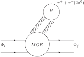
Figure 1:

II Formulation

II.1 The transition width

The theoretical framework about the QCD Multiploe Expandsion method is well established in RefsYK1 ; K2 ; Y1 ; K1 , and all the corresponding formulas are presented in their series of papers. Here we only make a brief introduction to the formulas for evaluating the widths which we are going to employ in this work. In Refs.YK1 ; K2 the transition rate of a vector quarkonium into another vector quarkonium with a two-pion emission can be written as

$$\Gamma(n_{I}{}^{3}S_{1}\rightarrow n_{F}{}^{3}S_{1})=|C_{1}|^{2}G|f^{l,P_{I},P_{F}}_{n_{I},l_{I},n_{F},l_{F}}|^{2}$$ (1)

where $|C_{1}|^{2}$ is a constant to be determined and it comes from the hadronization of gluons into pions, $G$ is the phase space factor, $f^{l,P_{I},P_{F}}_{n_{I},l_{I},n_{F},l_{F}}$ is the overlapping integration over the concerned hadronic wave functions, their concrete forms were given in K2 as

$$f^{l,P_{I},P_{F}}_{n_{I},l_{I},n_{F},l_{F}}=\sum_{K}\frac{\int R_{F}(r)r^{P_{F}}R^{*}_{Kl}(r)r^{2}dr\int R^{*}_{Kl}(r^{\prime})r^{\prime P_{I}}R_{I}(r^{\prime})r^{\prime 2}dr^{\prime}}{M_{I}-E_{Kl}},$$ (2)

where $n_{I},n_{F}$ are the principal quantum numbers of initial and final states, $l_{I},l_{F}$ are the angular momenta of the initial and final states, $l$ is the angular momentum of the color-octet $q\bar{q}$ in the intermediate state, $P_{I},P_{F}$ are the indices related to the multipole radiation, for the E1 radiation $P_{I},P_{F}$=1 and $l=1$. $R_{I},R_{F}$ and $R_{Kl}$ are the radial wave functions of the initial and final states, $M_{I}$ is the mass of initial quarkonium and $E_{Kl}$ is the energy eigenvalue of the intermediate hybrid state.

II.2 The $\bar{\chi}^{2}$ method

The standard method adopted in analyzing data and extracting useful information is minimizing the $\bar{\chi}^{2}$ and in our work, we hope to obtain the model parameters. When calculating $\bar{\chi}^{2}$, we would involve as many as possible experimental measurements to make the fitted parameters more reasonable. Here we adopt the form of $\bar{\chi}^{2}$ defined in chi as

$$\bar{\chi}^{2}=\sum_{i}\frac{(W^{th}_{i}-W^{exp}_{i})^{2}}{(\Delta W^{exp}_{i})^{2}},$$ (3)

where $i$ represents the i-th channel, $W^{th}_{i}$ is the theoretical prediction on the width of channel $i$, $W^{exp}_{i}$ is the corresponding experimentally measured value, $\Delta W^{exp}_{i}$ is the experimental error.

$W^{th}_{i}$ will be calculated in terms of the potential models with several free parameters which are described in the following subsections, thus $W^{th}_{i}$ is a function of the parameters. By minimizing $\bar{\chi}^{2}$, we would expect to determine the model parameters. Some details of our strategy will be depicted in subsection E.

II.3 The phenomenological potential for the initial and final quarkonia

In this work, we adopt two different potentials for the initial and final heavy quarkonia and the intermediate hybrid states.

The Cornell potential cornell is the most popular potential form to study heavy quarkonia. The potential reads as

$$V(r)=-\frac{\kappa}{r}+br,$$ (4)

usually in the literature many authors prefer to use $\alpha_{s}$ instead of $\kappa$ and it has a relation $\kappa=\frac{4\alpha_{s}(r)}{3}$, and $\alpha_{s}(r)$ can be treated as a constant for the $\bar{b}b$ and $\bar{c}c$ quarkonia.

The modifed Cornell potential: It may be more reasonable to choose a modified Cornell potential which includes a spin-related term ss , and the potential takes the form

$$V(r)=-\frac{\kappa}{r}+br+V_{s}(r)+V_{0},$$ (5)

where the spin-related term $V_{s}$ is,

$$V_{s}=\frac{8\pi\kappa}{3m_{q}^{2}}\delta_{\sigma}(r)\overrightarrow{S}_{q}\cdot\overrightarrow{S}_{\bar{q}}$$

with

$$\delta_{\sigma}(r)=(\frac{\sigma}{\sqrt{\pi}})^{3}e^{-\sigma^{2}r^{2}},$$

and $V_{0}$ is the zero-point energy,( in Ref.ss it was set to be zero), here we do not priori-assume it to be zero, but fix it by fitting the spectra of heavy quarkonia.

II.4 The potential for hybrids

The intermediate state as discussed above is a hybrid state $|q\bar{q}g>$ and we need to obtain the spectra and wave-functions of the ground state and corresponding radially excited states. Yan and Kuang used the phenomenological potential given by Buchmüller and Tye BT to evaluate the mass of the ground state of hybrid, instead, in our work, we take some effective potential models which are based on the color-flux-tube model.

Generally hybrids are labelled by the right-handed($n_{m}^{+}$) and left-handed($n_{m}^{-}$) transverse phonon modes

$$N=\sum_{m=1}^{\infty}m(n_{m}^{+}+n_{m}^{-}),$$

and a characteristic quantity $\Lambda$ as

$$\Lambda=\sum_{m=1}^{\infty}(n^{+}_{m}-n^{-}_{m}).$$

All the details about the definitions and notations can be easily found in literatureIsgur ; Swanson ; Allen ; Buisseret ; Szczepaniak ; Bali .

Various groups suggested different potential forms for the interaction between the quark and antiquark in the hybrid state. We label them as Model 1, 2 and 3 respectively.

In this work, we employ three potentials which are:

Model 1 was suggested by Isgur and Paton Isgur as

$$V(r)=-\frac{\kappa}{r}+br+\frac{\pi}{r}(1-e^{-fb^{1/2}r})+V_{0}.$$ (6)

Model 2: Swanson and SzczepaniakSwanson think that the Coulomb term in model 1 is not compatible with the lattice results, so that they suggested an alternative effective potential as

$$V(r)=br+\frac{\pi}{r}(1-e^{-fb^{1/2}r}).$$ (7)

To get a better fit to data, we add the zero-point energy $V_{0}$ into Eq.(7),

$$V(r)=br+\frac{\pi}{r}(1-e^{-fb^{1/2}r})+V_{0}.$$ (8)

Model 3: In model 1, the Coulomb piece is not proper, because the quark and antiquark in the hybrid reside in a color-octet instead of a singlet (the meson case), the short-distance behavior should be repulsive (it is determined by the sign of the expectation value of the Casimir operator in octet). Thus Allen $et\,al$ suggested the third model Allen and the corresponding potential form is

$$V(r)=\frac{\kappa}{8}+\sqrt{(br)^{2}+2\pi b}+V_{0}.$$ (9)

Because in these forms the authors do not consider the spin-related term (which we name as $V_{s}$.), we can modify the potential by adding a spin-related term $V_{s}$, then the potential becomes:

$$V(r)=V_{i}+V_{s}.$$ (10)

By this modification, one can investigate the spin-splitting effects. Generally, $V_{s}$ should have the same form as that in (5).

II.5 Our strategy

The strategy of this work is that we will determine the concerned parameters in the potential (Eqs.(6), (8), (9) and Eq.(10)) by fitting the data of heavy quarkonia transitions.

To obtain the concerned parameters in the potentials (Eqs.(6), (8), (9) and (10)) which specify the hybrids sates, we use the method of minimizing $\bar{\chi}^{2}$ defined in (3). Concretely, in Eq.(3), $W^{th}_{i}$ is a function of the parameters $\kappa,\;f,\;b,\;V_{0}$ and $|C_{1}|^{2}$, and following Ref.Isgur , we set $f=1$, therefore $\bar{\chi}^{2}$ is also a function of those parameters. Minimizing $\bar{\chi}^{2}$, one can fix the values of the corresponding parameters. Still for simplifying our complicated numerical computations, we choose a special method, namely, we first pre-set a group of the parameters, and we calculate the hybrid spectra and wave-functions by solving the Schrödinger equation, then we determine $|C_{1}|^{2}$ in Eq.(1) in terms of the well measured rate of $\psi(2S)\rightarrow J/\psi\,\pi\,\pi$. With this $|C_{1}|^{2}$ as a pre-determined value or say, a function of other parameters, we minimize $\bar{\chi}^{2}$ to fix the values of the rest of parameters $\kappa,\;b,\;V_{0}$.

With all the parameters being fixed, we can determine the mass spectra of the hybrids which serve as the intermediate states in the transitions of $\psi(ns)(\Upsilon(ns))\rightarrow\psi(ms)(\Upsilon(ms))+\pi\pi$. It is noted that the spectra determined in this scheme are not really the masses of physical states, unless the hybrids do not mix with regular quarkonia. In other words, we would determine a diagonal element of the mass Hamiltonian matrix, whose diagonalization would mix the hybrid and quarkonium and then determine the eigenvalues and eigen-functions corresponding to the physical masses and physical states which are measured in experiments.

III Numerical results

To determine the model parameters in the potential, we need to fit the spectra of $\psi(ns)$, $\eta_{c}(1s)$, $\eta_{c}(2s)$ and $\Upsilon(ns)$ and in this work, we only concern the ground states and radially excited states of $c\bar{c}$, $b\bar{b}$ and $c\bar{c}g$, $b\bar{b}g$ systems.

III.1 Without the spin-related term $V_{s}$

The potentials for quarkonia (Eq.(4)) and hybrid (Eq.(6) (model 1), Eq.(8) (model 2) and Eq.(9) (model 3)) do not include the spin-related term. In this work, we adopt the Cornell potential to calculate the spectra and wavefunctions of the regular heavy quarkonia. The concerned parameters in the Cornell potential have been given in literature as for the $c\bar{c}$ mesons, $\kappa=0.52,\;b=0.18\rm{GeV^{2}},\;m_{c}=1.84$ GeV, whereas for the $b\bar{b}$ mesons, $\kappa=0.48,\;b=0.18\rm{GeV^{2}},\;m_{b}=5.17$ GeVYK1 ; cornell . It is also noted that to meet the measured spectra of charmonia and bottonia a zero-point energy $V_{0}$ is needed.

The potential for the hybrid takes three possible forms which are shown in Eq.(6), (8) and (9). We keep the values $m_{c}=1.84$ GeV, $m_{b}=5.17$ GeV which are obtained by fitting the spectra of regular quarkonia $|b\bar{b}>\;(\Upsilon(ns))$ and $|c\bar{c}>\;(\psi(ns))$ with the potential (4), but need to gain the values of the relevant parameters $\kappa$, b and $V_{0}$ etc. by minimizing $\bar{\chi}^{2}$ for the decays $\psi(ns)(\Upsilon(ns))\to\psi(ms)(\Upsilon(ms))+\pi\pi$. According to the measured value for $\Gamma(\psi(2S)\rightarrow J/\psi\,\pi\,\pi)$:

$$\Gamma_{tot}(\psi(2S))=337\pm 13\rm{keV}$$

$$B(\psi(2S)\rightarrow J/\psi\pi^{+}\pi^{-})=(31.8\pm 0.6)\%$$

$$B(\psi(2S)\rightarrow J/\psi\pi^{0}\pi^{0})=(16.46\pm 0.35)\%$$

we express $C_{1}^{2}$ as a function of the potential parameters which exist in the three potentials ( Eqs.(6), (8) or (9)) and will be determined. It is noted that $C_{1}^{2}$ is a factor related to the hadronization of gluons into two pions, so should be universal for both $\psi$ and $\Upsilon$ decays. The parameters in the potentials are also universal for the $\bar{b}b$ and $\bar{c}c$ cases except the masses are different.

Then for $\Gamma(\Upsilon(nS)\to\Upsilon(ms)+\pi\pi)$ ($m<n$), we calculate $W^{th}_{i}$ in terms of the three potential forms. The corresponding experimental values and errors are $W^{exp}_{i}$ and $\Delta W^{exp}_{i}$ given in the references which are shown in Table 1.

Table 1: transition rate of $\Upsilon(nS)\to\Upsilon(ms)+\pi\pi$, (in unit of keV)

decay mode	Model 1	Model 2	Model 3	Experiment data
$\Upsilon(2S)\rightarrow\Upsilon(1S)\pi\pi$	9.36	9.28	8.69	$12.0\pm 1.8$
$\Upsilon(3S)\rightarrow\Upsilon(1S)\pi\pi$	1.81	1.67	1.85	$1.72\pm 0.35$
$\Upsilon(3S)\rightarrow\Upsilon(2S)\pi\pi$	0.86	0.76	0.86	$1.26\pm 0.40$
$\Upsilon(4S)\rightarrow\Upsilon(1S)\pi\pi$	3.87	3.43	4.14	$3.7\pm 0.6\pm 0.7$ Belle
$\Upsilon(4S)\rightarrow\Upsilon(2S)\pi\pi$	1.83	0.2	1.44	$2.7\pm 0.8$ 4s2s

By minimizing $\bar{\chi}^{2}$ (eq.(3)), we finally get the potential parameters $\kappa,\;b$ and $V_{0}$ and the resultant $\bar{\chi}^{2}$=4.42 for model 1, 13.69 for model 2 and 7.26 for model 3 . Then we obtain $|C_{1}|^{2}=100.39\times 10^{-6}$ for model 1, $259.24\times 10^{-6}$ for model 2, and $121.78\times 10^{-6}$ for model 3, the other parameters are listed in the following table (Table2).

Table 2: potential parameters for hybrid

	$\kappa$	$b$(GeV2)	$V_{0}$(GeV)
Model 1	0.43	0.19	-0.85
Model 2	-	0.15	-0.43
Model 3	0.59	0.19	-0.85

With these potential parameters, we solve the Schrödinger equation to obtain the masses of ground hybrid states of $|c\bar{c}g>$ and $|b\bar{b}g>$ (Table 5). It is noted that the resultant spectra depend on the potential forms. We will discuss this problem in the last section.

Table 3: the mass of hybrids(in units of GeV)

	Model 1	Model 2	Model 3
$|c\bar{c}g>$	4.099	4.549	4.226
$|b\bar{b}g>$	10.560	11.137	10.789

We also make a prediction on the rates which have not been measured yet(Table IV).

Table 4: prediction(in units of KeV)

decay mode	Model 1	Model 2	Model 3
$\Upsilon(4S)\rightarrow\Upsilon(3S)\pi\pi$	0.60	0.57	0.61
$\psi(3S)\rightarrow\psi(2S)\pi\pi$	14.96	14.45	14.83
$\psi(3S)\rightarrow\psi(1S)\pi\pi$	589.91	72.34	424.22

It is noted that values of $\Gamma(\psi(3S)\rightarrow\psi(1S)\pi\pi)$ predicted by models 1, 2 and 3 are quite apart, while $\Gamma(\Upsilon(4S)\rightarrow\Upsilon(3S)\pi\pi)$ and $\Gamma(\psi(3S)\rightarrow\psi(2S)\pi\pi)$ predicted by all the three models are close.

III.2 Comparison with the lattice results

To make sense, it would be helpful to compare the results obtained in our phenomenological work with the lattice results which are supposed to include both perturbative and non-perturbative QCD effects. Below we show comprehensive comparisons of our potentials with the lattice results.

Following Refs.Swanson ; Allen ; Buisseret ; Szczepaniak ; lattice , the potentials shown in Fig.2 are specially scaled by $V_{\Sigma_{g}^{+}}(2r_{0})$ which is the potential for $\Sigma_{g}^{+}$ (N=0) at $2r_{0}=5\;{\rm GeV}^{-1}$ (for the vertical axis of Fig.2.).

In the three graphs of Fig. 2, we present comparisons of the three potentials (models, 1,2 and 3) with the parameters fixed in last subsections with the lattice results. In the graphs, the dots are the lattice values lattice .

It is emphasized that we obtain the potential by minimizing $\bar{\chi}^{2}$ of the data on $\psi(ns)(\Upsilon(ns))\to\psi(ms)(\Upsilon(ms))+\pi\pi$, but do not fit the lattice values. Then our results, especially the third potential coincides with the lattice results extremely well. It may indicate that the physics description adopted in this scenario is reasonable. It is also noted that by model 1, the short-distance behavior of the potential is attractive and obviously distinct from the lattice results. This discrepancy was discussed above that the quark-antiquark system in hybrid should be a color-octet and short-distance interaction should be repulsive. The second potential (model 2) have the same trend as the lattice results, but have obvious deviations (see the graph 2 of Fig. 2).

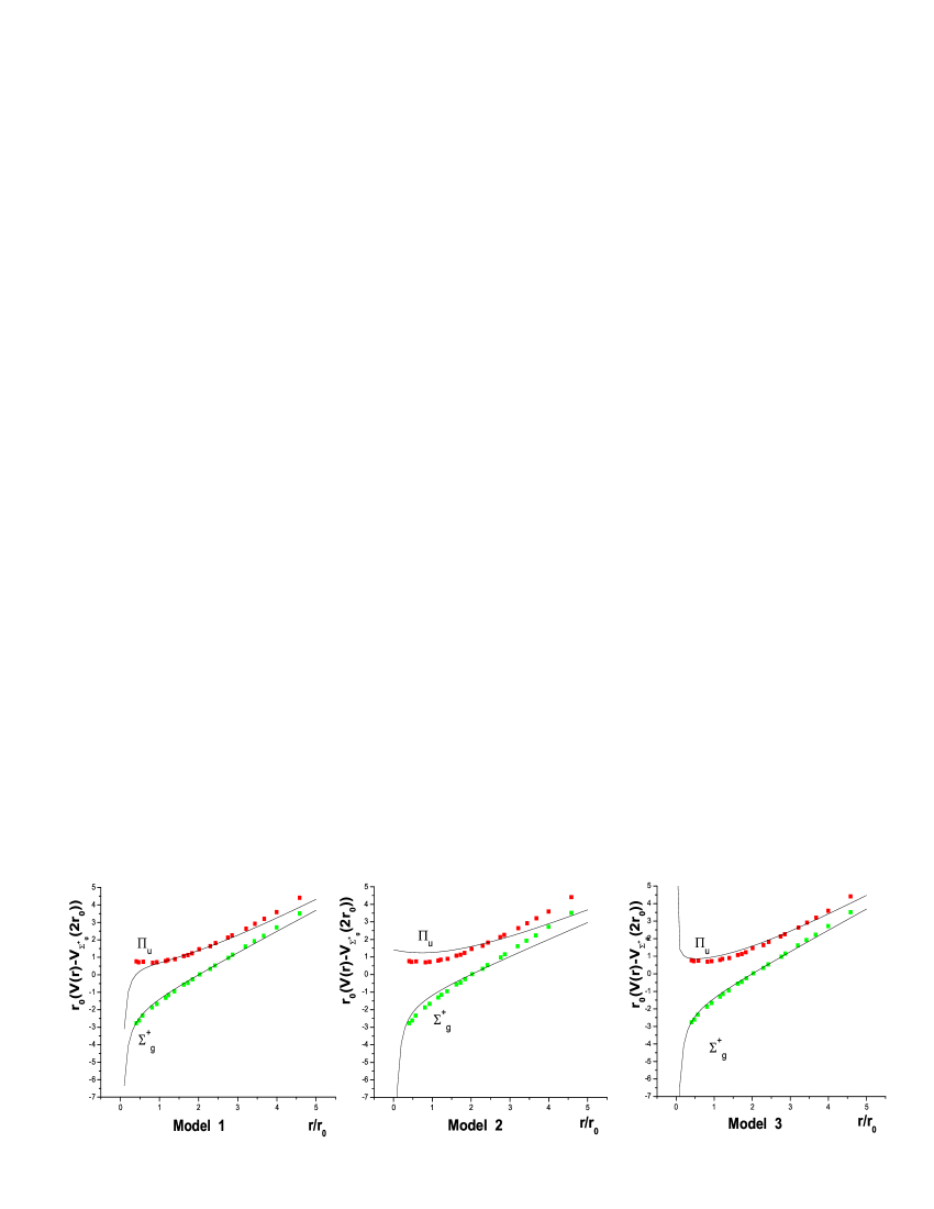
Figure 2:

III.3 With the spin-related terms $V_{s}$

For the regular quarkonia we adopt the non-relativistic potential(NR) Eq.(5) ss . Since we add a zero-point energy $V_{0}$ in the potential which can be seen as another free parameter (it is the same for both $c\bar{c}$ and $b\bar{b}$ quarkonia), we re-fit the spectra of the quarkonia to obtain the corresponding potential parameters in Eq.(5). We list the resultant values of the parameters in Table 5. In Table 6, we present the fitted spectra of $c\bar{c}$ and for a comparison, we also include the results given in Ref.ss in the table.

Table 5: potential parameters for $c\bar{c}$

$\kappa$	$b$(GeV2)	$m$(GeV)	$\sigma$(GeV${}^{2})$	$V_{0}$(GeV)
0.67	0.16	1.78	1.6	-0.6

Table 6: Eignvalues for $c\bar{c}$ in GeV

	$J/\psi$	$\psi(2S)$	$\psi(3S)$	$\psi(4S)$	$\eta_{c}(1S)$	$\eta_{c}(2S)$
Refss	3.090	3.672	4.072	4.406	2.982	3.630
this work	3.097	3.687	4.093	4.433	2.971	3.634

For the $b\bar{b}$ quarkonia, the corresponding parameters obtained by fitting data are listed in Table 7.

Table 7: potential parameters for $b\bar{b}$

$\kappa$	$b$(GeV2)	$m$(GeV)	$\sigma$(GeV${}^{2})$)	$V_{0}$(GeV)
0.53	0.16	5.13	1.7	-0.60

By the parameters we predict $m_{\eta_{b}}=9.434$ GeV, which is consistent with that given by bb .

Then we turn to the hybrid intermediate states.

For the hybrids, by the observation made in the previous subsection one can conclude that the third potential (model 3) better coincides with the lattice results, therefore, in this subsection when we include the spin-related term to discuss spin-splitting case, we only adopt the third potential Eq.(9). It is reasonable to keep the values of $m_{c}$, $m_{b}$ and $\sigma$ to be the same as that we determined for pure $q\bar{q}$ quarkonia and we also set $f=1$. Then following our strategy discussed in previous subsections, we obtain the potential parameters which are listed in the following table.

Table 8: potential parameters for hybrid

	$\kappa(c\bar{c}g)$	$\kappa(b\bar{b}g)$	$b$(GeV2)	$V_{0}$(GeV)
the best fitted values	0.54	0.40	0.24	-0.80

The fitted values and some predictions are also listed in Tables 9 and 10. We obtain

$$|C_{1}|^{2}=182.12\times 10^{-6},\qquad$$

the mass of hybrids are 4.351GeV, 4.333 GeV for the spin-triplet and spin-singlet $c\bar{c}$ in the hybrid and 10.916GeV, 10.913GeV for the spin-triplet and singlet $b\bar{b}$ respectively. Because of including the spin-related term, the “ground states” with the $q\bar{q}$ (q=b or c) being in different spin structures would be slightly split.

One can observe that the predicted $\Gamma(\Upsilon(4S)\rightarrow\Upsilon(3S)\pi\pi)$ and $\Gamma(\psi(3S)\rightarrow\psi(2S)\pi\pi)$ are slightly smaller than that predicted in the models without the spin-related term, the future experiments may shed some light on it, namely getting better understanding on the mechanisms which one can describe the hybrid structure better.

We also calculate the transition rate of $\eta^{\prime}_{c}\rightarrow\eta_{c}+\pi+\pi$, our result is almost triple that obtained in Ref.Y1 and it can be tested by the future experiments.

Table 9: $\Upsilon$  transition(in units of keV)

decay mode	widths (fit)
$\Upsilon(2S)\rightarrow\Upsilon(1S)\pi\pi$	8.73
$\Upsilon(2S)\rightarrow\Upsilon(1S)\pi\pi$	1.94
$\Upsilon(3S)\rightarrow\Upsilon(2S)\pi\pi$	0.69
$\Upsilon(4S)\rightarrow\Upsilon(1S)\pi\pi$	4.10
$\Upsilon(4S)\rightarrow\Upsilon(2S)\pi\pi$	1.88

It is noted that since we minimize $\bar{\chi}^{2}$, the decay widths that we obtain are different from the central values of the measured quantities. We list the widths we finally obtained in the table 9.

Table 10: prediction(in units of keV)

decay mode	widths of predition
$\Upsilon(4S)\rightarrow\Upsilon(3S)\pi\pi$	0.36
$\psi(3S)\rightarrow\psi(2S)\pi\pi$	8.84
$\psi(3S)\rightarrow J/\psi\pi\pi$	12.38
$\eta_{c}(2S)\rightarrow\eta_{c}\pi\pi$	335.66

IV Our conclusion and discussion

Search for exotic states which are allowed by the SU(3) quark model and QCD theory is very important for our understanding of the basic theory, but so far such states have not been found (or not firmly identified), thus it becomes an attractive task in high energy physics. No doubt, direct measurements on such exotic states would provide definite information on them, however, it seems that most of the mysterious states mix with mesons and baryons which have regular quark structures. Since they are hidden in the mixed states, they are not physical states and do not have physical masses, and it makes a clear identification of such exotic states very difficult. In other words, they may only serve as a component of physical states. Even though, some phenomenological models, such as the color-flux-tube model, the bag model and the potential model etc., are believed to properly describe their properties and determine their “masses”, in fact, if they mix with the regular mesons or baryons, the resultant masses are only the diagonal elements of the Hamiltonian matrix. For example, in the potential model, by solving Schrödinger equation, one obtains the eigen-energy and wave function, he only gets the element $E_{11}=_{hyb}<\phi|H_{hyb}|\phi>_{hyb}$, where the subscript “hyb” denotes the quantities corresponding to hybrids. Meanwhile, there is $E_{22}=_{reg}<\phi|H_{reg}|\phi>_{reg}$ corresponding to the regular quark structure. If the two eigen-states are not far located, they may mix with each other and provide an extra matrix element to the hamiltonian matrix, as $E_{12}=E_{21}^{*}=_{hyb}<\phi|H_{mix}|\phi>_{reg}$. Unfortunately, there is not a reliable way to calculate the mixing matrix element. One may expect to gain definite information about the hybrid states and maybe starting from there he can further study the mechanism of the mixing.

The theoretical framework established by Yan and Kuang confirms that the intermediate states between two pion-emissions in the transition $\psi(ns)(\Upsilon(ns))\rightarrow\psi(ms)(\Upsilon(ms))+\pi\pi$, are hybrids which contain a quark-antiquark pair in color octet, and an extra valence gluon. Based on the color-flux-tube model, in 80’s of last century Isgur and Paton suggested a potential model for the hybrid, and this greatly simplifies the discussion about hybrids and may offer an opportunity to study the regular quarkonium and hybrid in a unique framework. After their work, several other groups also proposed modified potentials to make a better description on the hybrid states. When Yan and Kuang studied the transitions, there were not many data available, i.e. most of the channels were not measured yet. Therefore they assumed that $\psi(4.03)$ as the ground state of charmed hybrids $|c\bar{c}g>$ and estimated the transition rates. Thanks to the great achievements of the Babar and Belle collaborations, many such modes are measured with appreciable accuracy. Based on the experimental data and the theoretical framework established by Yan and Kuang, we minimize the $\bar{\chi}^{2}$ to obtain the model parameters in the potential for hybrid, and with them, we can estimate the masses of the ground states of hybrids. The theory of the QCD multi-expansion is based on the assumption that the hadronization of the emitted gluons can be factorized from the transition of $\Upsilon(ns)(\psi(ns))\to\Upsilon(ms)(\psi(ms))$. In fact, this factorization may be not complete if the non-perturbative QCD effects are invloved, namely the higher twist contribution may somehow violate the factorization. However, as long as the non-perturbative QCD effects are not too strong, this approximation should be acceptable within a certain tolerance range. Moreover, in our study, the non-factorization effects are partly involved in the parameter $|C_{1}|^{2}$ of Eq. (1), and in our scheme it is also one of the free parameters which are fixed by fitting data. Indeed, it is implicitly assumed that $|C_{1}|^{2}$ is universal for all the processes, and it may cause some error. But it is believed that since the energy range does not change drastically, the error should controllable.

In the calculations, we adopt the Cornell potential for the color-singlet $q\bar{q}$ (q=b or c) system and the potentials suggested by Isgur and Paton (model 1)Isgur , by Swanson and Szczepaniak (model 2) Swanson and by Allen $et\,al$ (model 3) Allen to deal with the color-octet $q\bar{q}$ system, we add a spin-related term to the potential for hybrid (model 3 only) to investigate possible spin-splitting effects. The numerical results are slightly different when this term is introduced. The masses of the ground state hybrids are 4.23 GeV for $|c\bar{c}g>$ and 10.79 GeV for $|b\bar{b}g>$ which are estimated in terms of model 3. When the spin-related term is included, the results change to 4.351 GeV, 4.333 GeV for the spin-triplet and spin-singlet $c\bar{c}$ in the hybrid and 10.916 GeV, 10.913 GeV for the spin-triplet and singlet $b\bar{b}$ respectively. In other two models, the results are slightly different. Indeed as aforementioned, a comprehensive comparison of the results with the lattice values, one may be convinced that the model 3 may be the best choice at present. All the obtained masses are different from the physical states measured in experiments, and it may imply that the hybrids mix with regular mesons.

There are more data in the b-energy range than in charm-energy region. In fact, when we use the same method to calculate the transition $\psi(ns)\rightarrow\psi(ms)+\pi\pi$, with n and m being widely apart (say n=4, m=1 etc.), the theoretical solutions are not stable and uncertainties are relatively large. It indicates that there are still some defects in the theory which would be studied in our future works. Moreover, recently Shen and Guo shen studies the processes in terms of the chiral perturbation theory and considered the final state interaction to fit the details of the $\pi\pi$ energy and angular distributions.

The transition of higher excited states of quarkonia into lower ones (including the ground state) without flavor change but emitting photon or light mesons is believed to offer rich information on the hadron structure and governing dynamics, especially for the heavy quarkonia physics, for example, Brambilla $et$ $al$.Brambilla studied the quarkonium radiative decays which are realized via electromagnetic interactions.

Our studies indicate that the transitions of $\psi(ns)(\Upsilon(ns))\rightarrow\psi(ms)(\Upsilon(ms))+\pi\pi$ may provide valuable information about the hybrid structures which have so far not been identified in experiments yet.

Since we use the method of minimizing $\bar{\chi}^{2}$ to achieve all the parameters in the potential model for hybrids, it certainly brings up some errors. It is a common method for both experimentalists and theorists to analyze data and obtain useful information. Definitely, the more data are available, the more accurate the results would be. Therefore more data are very necessary, especially the data on the $\psi$ families which are one of the research fields of the BES III and CLEOc.

Acknowledgements:

This work is supported by the National Natural Science Foundation of China (NNSFC), under the contract No. 10475042.

References

- (1) K. Gottfried, Phys. Rev. Lett. 40, 598(1978).
- (2) Y. Kuang and T. Yan, Phys. Rev. D 24, 2874(1981).
- (3) Y. Kuang , Front. Phys. China 1, 19(2006).
- (4) T. Yan, Phys. Rev. D 22, 1652(1980).
- (5) Y. Kuang, Y. Yi and B. Fu, Phys. Rev. D 42, 2300(1990).
- (6) L. Brown and R. Cahn, Phys. Rev. Lett. 35, 1(1975).
- (7) W. Buchmller and H. Tye, Phys. Rev. Lett. 44, 850(1980).
- (8) W. Yao ., [Partical Data Group], J. Phys. G 33, 1(2006).
- (9) B. Aubert ., [BaBar Collaboration], Phys. Rev. Lett. 96, 232001(2006).
- (10) A. Sokolov ., [Belle Collaboration], hep-ex/0611026.
- (11) N. Isgur and J. Paton, Phys. Rev. D 31, 2910(1985).
- (12) E. Swanson and A. Szczepaniak, Phys. Rev. D 59, 014035(1999).
- (13) T. Allen, M. Olsson and S. Veseli, Phys. Lett. B 434, 110(1998).
- (14) C. Chiang, M. Gronau, J. Rosner and D. Suprun, Phys. Rev. D 70, 034020(2004).
- (15) E. Eichten, K. Gottfried, T. Kinashita, K. Lane and T. Yan , Phys. Rev. D 17, 3090 (1978); , D 21, 203(1980).
- (16) T. Barnes, S. Godfrey and E. Swanson , Phys. Rev. D 72, 054026(2005) .
- (17) F. Buisseret and V. Mathieu, Eur. Phys. J. A 29, 343(2006).
- (18) A. Szczepaniak and P. Krupinski, Phys. Rev. D 73, 116002(2006); P. Guo, A. Szczepaniak G. Galata, A. Vassallo and E. Santopina, arXiv:0707.3156 [hep-ph].
- (19) G. Bali and A. Pineda, Phys. Rev. D 69, 094001(2004).
- (20) K. Juge, J. Kuti and C. Morningstar, Nucl. Phys. (Proc. Suppl.) B 63, 326(1998); Phys. Rev. Lett. 90, 161601 (2003).
- (21) G. Hao, Y. Jia, C. Qiao, and P. Sun, Phys. Rev. D 75, 035010(2007); D. Ebert, R. Faustov and V. Galkin, Phys. Rev. D 67, 014027(2003); S. Recksiegel and Y. Sumino, Phys. Lett. B 578, 369(2004); B. Kniehl, A. Penin, A. Pineda, V. Smirnov and M. Steinhauser, Phys. Rev. Lett. 92, 242001(2004); A. Gray, I. Allison, C. Davies, E. Gulez, G. Lepage, J. Shigemitsu and M. Wingate, Phys. Rev. D 72, 094507(2005).
- (22) F. Guo, P. Shen, H. Chiang and R. Ping, Nucl. Phys. A761, 269(2005); F. Guo, P. Shen and H. Chiang, Phys. Rev. D74, 014011(2006); F. Guo, P. Shen, H. Chiang and R. Ping, hep-ph/0601120.
- (23) N. Brambilla, Y. Jia and A. Vairo, Phys. Rev. D 73, 054005(2006); N. Brambilla ., hep-ph/0412158.