Berry’s phase for coherent states of Landau levels

Abstract

The Berry’s phase for coherent states and squeezed coherent states of Landau levels are calculated. Coherent states of Landau levels are interpreted as a result of a magnetic flux moved adiabaticly from infinity to a finite place on the plane. The Abelian Berry’s phase for coherent states of Landau levels is an analogue of the Aharonov-Bohm effect. Moreover, the non-Abelian Berry’s phase is calculated for the adiabatic evolution of the magnetic field $B$.

I introduction

Since the famous work of Berry 84MVB (1), the geometric phase has been widely investigated and its generalizations have been made in many ways 83BS (2)84WZ (3)87AA (4)88SB (5). Recently much concern has been concentrated on the geometric phase of entangled states as well as mixed states EP00 (6)MP00 (7). Coherent state is an important physical concept both theoretically and experimentally g1963 (8)creview (9). It can be generated from an arbitrary reference state, and in this Brief Report Landau levels are chosen to be such reference states. Though coherent states of Landau level have been studied in Refs. LPR (10)SU11 (11) and Berry’s phase for coherent states as well as squeezed coherent states of a one-dimensional harmonic oscillator has been illustrated in Ref. 87CSS (12), Berry’s phase for coherent states of Landau levels which is highly degenerate and with an additional parameter, i.e., the magnetic field $B$, is still worthy of further investigation.

This paper is organized as follows. In Sec. II, we show how to get the coherent states of Landau levels, and these states can be regarded as a result of a magnetic flux moved adiabaticly from infinity to a finite place on the plane. In Sec. III, we calculate the Abelian and non-Abelian Berry’s phase for coherent states of Landau levels. The Abelian Berry’s phase is just like an alternative version of the Aharonov-Bohm (AB) effect; the difference between them is that in our case the cyclic motion of the magnetic flux results in the phase shift. In Sec. IV, we provide the explicit form of the Hamiltonian and Berry’s connections for squeezed coherent states of Landau levels. Conclusion and discussion are made in the last section.

II Coherent states of Landau levels

The motion of a free electron in a two-dimensional $xy$-plane in a static magnetic field along the $z$-direction is described by the following Hamiltonian

$$H=\frac{\hbar^{2}}{2\mu}[(p_{x}+\frac{e}{c}A_{x})^{2}+(p_{y}+\frac{e}{c}A_{y})^{2}],$$ (1)

where $\mu$ is the mass of the electron, $\hbar$ is the Planck constant, $-e$ is the electron charge, $c$ is the speed of light in the vacuum, $p_{x}$ and $p_{y}$ are the linear momentums, $A_{x}$ and $A_{y}$ are vector potentials of the magnetic field satisfying $\partial_{x}A_{y}-\partial_{y}A_{x}=B$. For simplicity the Zeeman’s term is not included.

We introduce the following operators

$$\pi_{x}=p_{x}+\frac{e}{c}A_{x},\;\pi_{y}=p_{y}+\frac{e}{c}A_{y},\;\pi_{\pm}=\pi_{x}\pm i\pi_{y}.$$ (2)

from which one can form a pair of operators $b^{+}$ and $b$ which satisfy the commutation relation $[b,b^{+}]=1$:

$$b=\sqrt{\frac{c}{2\hbar eB}}\pi_{-},\;\;b^{+}=\sqrt{\frac{c}{2\hbar eB}}\pi_{+}.$$ (3)

In this case we can rewrite the Hamiltonian in a more simpler form

$$H_{0}=\hbar\omega(b^{+}b+1/2),$$ (4)

where $\omega=eB/c\mu$, and $b^{+}$, $b$ are raising and lowering operators between Landau levels with $b^{+}\left|n\right\rangle=\sqrt{n+1}\left|n+1\right\rangle$, $b\left|n\right\rangle=\sqrt{n}\left|n-1\right\rangle$. The energy of Landau levels is $E_{n}=\hbar\omega(n+1/2)$. One knows that Landau levels are highly degenerate. In the degenerate space of Landau levels we can introduce another pair of raising and lowering operators

$$a = \sqrt{\frac{c}{2\hbar eB}}\left(-p_{x}-ip_{y}+\frac{e}{c}A_{x}+i\frac{e}{c}A_{y}\right),$$

$$a^{+} = \sqrt{\frac{c}{2\hbar eB}}\left(-p_{x}+ip_{y}+\frac{e}{c}A_{x}-i\frac{e}{c}A_{y}\right).$$

We choose the symmetric gauge $A_{x}=-\frac{y}{2}B$ and $A_{y}=\frac{x}{2}B$, and then $a$, $a^{+}$ are commutative with $b$, $b^{+}$ and $[a,a^{+}]=1$. Therefore the Hamiltonian commutes with $a$ and $a^{+}$. The ground state is defined as $\left|0,0\right>=\sqrt{Be/(2\pi c\hbar)}\exp[-Be(x^{2}+y^{2})/(4c\hbar)]$, and all other eigenstates of this system can be generated from $\left|0,0\right>$ state with raising operators $\left|n,m\right>=\frac{1}{\sqrt{n!m!}}b^{+^{n}}a^{+^{m}}\left|0,0\right>$. The states $\left|n,m\right>$ are also orthogonal and normalized bases for this system. States with the same $n$ are in the same energy level, and states with the same $n$ but different $m$ stand for the different degenerate states on the same energy level.

The coherent states of Landau levels are generated in the following way as in 87CSS (12):

$$\left|n(\alpha),m\right>=\exp(\alpha b^{+}-\alpha^{*}b)\left|n,m\right>,$$

where $\alpha=X_{1}+iX_{2}$. The Hamiltonian for the coherent states is:

$$H=D(\alpha)H_{0}D^{+}(\alpha)=\hbar\omega\left[(b^{+}-\alpha^{*})(b-\alpha)+\frac{1}{2}\right],$$ (5)

where $D(\alpha)=\exp(\alpha b^{+}-\alpha^{*}b)$, and the eigenstates of this Hamiltonian are always combinations of the degenerate states with the same energy:

$$\left|n(\alpha)\right>=\sum\limits_{m}f_{m}\left|n(\alpha),m\right>,$$ (6)

where $f_{m}$ are arbitrary complex numbers which make $\left|n(\alpha)\right>$ normalized. We put Eq. (3) back to Eq. (5), this would make the Hamiltonian easier to understand, we get

$$H=\frac{\hbar^{2}}{2\mu}[(\pi_{x}-\sqrt{\frac{2\hbar eB}{c}}X_{1})^{2}+(\pi_{y}+\sqrt{\frac{2\hbar eB}{c}}X_{2})^{2}].$$ (7)

We found that the magnetic vector potential is added by a constant vector potential. This can be regarded as a result of a magnetic flux perpendicular to the plane moving adiabaticly from infinitely far to a finitely far position on the plane. In the following we would like to show how we get the result.

We can assume that the added magnetic flux is a Gaussian form magnetic field centered $(x_{0},y_{0})$, $B^{\prime}=\frac{\Phi_{0}}{\pi\Delta^{2}}\exp\left[-\frac{(x-x_{0})^{2}+(y-y_{0})^{2}}{\Delta^{2}}\right]$, where $\Delta$ is refered to as the spread or standard deviation for the Gaussian function. And we may choose the symmetric gauge with respect to $(x_{0},y_{0})$, i.e., $\left.\nabla\cdot\mathbf{A}\right|_{x=x_{0},y=y_{0}}=0$, the nonsingular vector potential for this added magnetic field is

$$A^{\prime}_{x} = \frac{\Phi_{0}\{\exp[-\frac{(x-x_{0})^{2}+(y-y_{0})^{2}}{\Delta^{2}}]-1\}(y-y_{0})}{2\pi[(x-x_{0})^{2}+(y-y_{0})^{2}]},$$

$$A^{\prime}_{y} = -\frac{\Phi_{0}\{\exp[-\frac{(x-x_{0})^{2}+(y-y_{0})^{2}}{\Delta^{2}}]-1\}(x-x_{0})}{2\pi[(x-x_{0})^{2}+(y-y_{0})^{2}]}.$$ (8)

One may observe that $B^{\prime}$ has nothing to do with the Hamiltonian (1) when $x_{0},y_{0}\rightarrow\infty$. Now we assume that the electron in the plane is in a certain eigenstate, for example, $|0,0\rangle$, in this case the electron is localized near the origin because of $\langle x\rangle=\langle 0,0|x|0,0\rangle=\langle y\rangle=0$, $\langle x^{2}+y^{2}\rangle=2c\hbar/Be$. Let $\Delta>\langle\sqrt{x^{2}+y^{2}}\rangle$, so when the flux moves adiabaticly to a place $(x_{0},y_{0})$ which is finitely far from the electron (i.e. $x_{0},y_{0}\gg\langle\sqrt{x^{2}+y^{2}}\rangle\simeq\sqrt{2c\hbar/Be}$), we assume that the electron is still distributed around the origin and $A^{\prime}_{x},\ A^{\prime}_{y}$ near the origin of the plane can be regarded as constants. Then the Hamiltonian for the electron will be of the form (7) with

$$X_{1}=\sqrt{\frac{e}{2\hbar Bc}}\frac{\Phi_{0}y_{0}[\exp\left(-\frac{x_{0}^{2}+y^{2}_{0}}{\Delta^{2}}\right)-1]}{2\pi(x_{0}^{2}+y_{0}^{2})},$$

$$X_{2}=\sqrt{\frac{e}{2\hbar Bc}}\frac{\Phi_{0}x_{0}[\exp\left(-\frac{x_{0}^{2}+y_{0}^{2}}{\Delta^{2}}\right)-1]}{2\pi(x_{0}^{2}+y_{0}^{2})}.$$ (9)

This modification of the Hamiltonian also corresponds to the following transformation $(x,y)\rightarrow(x+\delta x,y+\delta y)$, where

$$\delta x=\frac{\Phi_{0}x_{0}[\exp(-\frac{x_{0}^{2}+y_{0}^{2}}{\Delta^{2}})-1]}{\pi B(x_{0}^{2}+y_{0}^{2})},$$

$$\delta y=\frac{\Phi_{0}y_{0}[\exp(-\frac{x_{0}^{2}+y_{0}^{2}}{\Delta^{2}})-1]}{\pi B(x_{0}^{2}+y_{0}^{2})}.$$ (10)

So the state $\psi_{00}(x,y)=\left|0,0\right>$ will become $\psi_{00}(x+\delta x,y+\delta y)$. Since the distribution of the electron is near the origin, one also makes sure that $\delta x\ll x_{0},\ \delta y\ll y_{0}$.

The coherent states of Landau levels is nothing but the shifted eigenstates of Landau levels in the phase space, here we assume such a shift happens in real space $\psi_{00}(x,y)\rightarrow\psi_{00}(x+\delta x,y+\delta y)$. When the conditions above are satisfied, this assumption is reasonable. It is $B^{\prime}$ who causes this small shift. We may see from Eq. (II) that the direction of $B^{\prime}$, i.e., the sign of $\Phi_{0}$ is related to the direction of the shift. When $\Phi_{0}>0$ the shift is parallel to the direction of the flux, and vice versa. Interestingly, if the flux circles the electron once, the electron will also circle the origin in a much smaller loop once. This is the reason why the Berry’s phase emerged as we will show in the next section.

III Berry’s phase for coherent states of landau levels

We know that the Landau levels are highly degenerate, and so is the coherent states of Landau levels. Berry’s phase for degenerate states was presented in 84WZ (3) and may have a non-Abelian nature. We calculated the Berry’s connections as follows:

$$\left<n(\alpha),m\right|\partial_{X_{1}}\left|n^{\prime}(\alpha),m^{\prime}\right>=(-iX_{2})\delta_{n,n^{\prime}}\delta_{m,m^{\prime}}$$

$$\ \ \ +(\sqrt{n^{\prime}+1}\delta_{n,n^{\prime}+1}-\sqrt{n^{\prime}}\delta_{n,n^{\prime}-1})\delta_{m,m^{\prime}},$$

$$\left<n(\alpha),m\right|\partial_{X_{2}}\left|n^{\prime}(\alpha),m^{\prime}\right>=iX_{1}\delta_{n,n^{\prime}}\delta_{m,m^{\prime}}$$

$$\ \ \ +(i\sqrt{n^{\prime}+1}\delta_{n,n^{\prime}_{1}}+i\sqrt{n^{\prime}}\delta_{n,n^{\prime}-1})\delta_{m,m^{\prime}},$$

$$\left<n(\alpha),m\right|\partial_{B}\left|n^{\prime}(\alpha),m^{\prime}\right>=\frac{1}{2B}(\alpha\sqrt{m^{\prime}}\delta_{m,m^{\prime}-1}$$

$$\ \ \ -\alpha^{*}\sqrt{m^{\prime}+1}\delta_{m,m^{\prime}+1})\delta_{n,n^{\prime}}$$

$$\ \ +\frac{1}{2B}\sqrt{n^{\prime}m^{\prime}}\delta_{n,n^{\prime}-1}\delta_{m,m^{\prime}-1}$$

$$\ \ -\frac{1}{2B}\sqrt{(n^{\prime}+1)(m^{\prime}+1)}\delta_{n,n^{\prime}+1}\delta_{m,m^{\prime}+1}.$$ (11)

In the degenerate space, i.e., between states with the same $n$, the Berry’s connections become

$$A^{m,m^{\prime}}_{X_{1}}=-iX_{2}\delta_{m,m^{\prime}},\ A^{m,m^{\prime}}_{X_{2}}=iX_{1}\delta_{m,m^{\prime}}$$

$$A^{m,m^{\prime}}_{B}=\frac{1}{2B}(\alpha\sqrt{m^{\prime}}\delta_{m,m^{\prime}-1}-\alpha^{*}\sqrt{m^{\prime}+1}\delta_{m,m^{\prime}+1}).$$

We found that $A_{X_{1}}$ and $A_{X_{2}}$ are Abelian. With the adiabatic theorem for degenerate states proved in AA (13) and to a higher order in BB (14), we know that the $|f_{m}|$ in Eq. (6) will not change during the arbitrary slow evolution of $X_{1}$ and $X_{2}$. Also because the Berry’s connections of $X_{1}$ and $X_{2}$ are Abelian, $f_{m}$’s will gain a Berry’s phase factor, which is the same of all $m$, after an adiabatic evolution in the $X_{1}$-$X_{2}$ plane. The Berry’s phase is

$$\gamma_{n} =i \oint_{C}\left<n(\alpha)\right|\partial_{X_{1}}\left|n(\alpha)\right>dX_{1}+\left<n(\alpha)\right|\partial_{X_{2}}\left|n(\alpha)\right>dX_{2}$$ (13)

$$= \oint_{C}X_{2}dX_{1}-X_{1}dX_{2}=-2S,$$

where $C$ is the path of the adiabatic evolution of $(X_{1},X_{2})$ in $X_{1}$-$X_{2}$ plane and $S$ is the area of $C$. This result appeared in 87CSS (12) for non-degenerate coherent states. The result is also the same as the phase in the paper PE00 (15). However, in our case it is the moving magnetic flux that moves the electron instead of a moving potential well.

With the interpretation in the above section, we can see from Eq. (II) that when the magnetic flux circles the electron for one loop, the $(X_{1},X_{2})$ will also enclose an area, and this gives the Berry’s phase. For example, we let $(x_{0},y_{0})$ moves around the origin in a circle with the radius $R$ for one loop. The Berry’s Phase will be

$$\gamma^{\prime}=-2S^{\prime}=-\frac{e\Phi_{0}^{2}(1-e^{-R^{2}/{\Delta}^{2}})^{2}}{4\pi\hbar cBR^{2}}.$$ (14)

This can be viewed as an alternative version of the AB effect. The different between them is that we move the magnetic flux instead of the electron.

One may see from Eq. (III) that $A^{m,m^{\prime}}_{B}$ is non-Abelian, so the change of $B$ will give non-Abelian Berry’s phase. As the non-Abelian Berry’s phase in such a system has not been shown in the literature before, in the following we would like to give a simple examples to illustrate it.

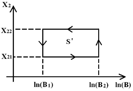
Figure 1: This is the loop of the adiabatic evolution in $X_{2}$-$\ln(B)$ plane. The magnetic field $B$ appears in Berry’s phase in the logarithm form.

We assume $X_{1}=0$ during the evolution and the other two parameters undergo the loop in Fig. 1. We can get the eigenvalues of matrix $A_{B}$ as $\varepsilon_{\xi}/(2B)$ and the corresponding eigenstates $\left|n(\alpha),\xi\right>$. The states before evolution Eq. (6) can be rewritten in the new base as

$$\left|n(iX_{21},t=0)\right>$$

$$=\sum\limits_{\xi}\left<n(iX_{21}),\xi\right|\left.n(iX_{21})\right>\left|n(iX_{21}),\xi\right>.$$ (15)

After the system undergoes an evolution as shown in Fig. 1, the state may become

$$\left|n(iX_{21},t=\tau)\right>$$

$$=\sum\limits_{\xi}e^{-i\varepsilon_{\xi}S^{\prime}}\left<n(iX_{21}),\xi\right|\left.n(iX_{21})\right>\left|n(iX_{21}),\xi\right>,$$ (16)

where $S^{\prime}$ is the area enclosed by $X_{2}$ and $\ln(B)$ as in Fig. 1. However, if $X_{1}\neq 0$, the calculation will involve path ordered integral and beome very complicated.

IV Berry’s phase for squeezed coherent states of Landau levels

The Hamiltonian for squeezed coherent state is

$$H=D(\alpha)S(\beta)H_{0}S^{+}(\beta)D^{+}(\alpha),$$ (17)

where $H_{0}$ is defined in Eq. (4), $\beta=re^{i\theta}$ and

$$S(\beta)=\exp(\frac{1}{2}\beta b^{+2}-\frac{1}{2}\beta^{*}b^{2}).$$ (18)

The eigenstates for this Hamiltonian, i.e., the squeezed coherent states are

$$\left|n(\alpha,\beta),m\right>=D(\alpha)S(\beta)\left|n,m\right>.$$ (19)

In the same way,we put Eq. (3) to Eq. (17), and we can get

$$H = \frac{1}{2\mu}\left\{e^{-2r}\left[\cos(\theta/2)\pi^{\prime}_{x}+\sin(\theta/2)\pi^{\prime}_{y}\right]^{2}\right.$$ (20)

$$\left.+e^{2r}\left[-\sin(\theta/2)\pi^{\prime}_{x}+\cos(\theta/2)\pi^{\prime}_{y}\right]^{2}\right\},$$

where $\pi^{\prime}_{x}=\pi_{x}-\sqrt{2\hbar eB/c}X_{1},\ \pi^{\prime}_{y}=\pi_{y}+\sqrt{2\hbar eB/c}X_{2}$. For $r=0$, Eq. (20) reduces to Eq. (7). For $r\neq 0$, one can see from this Hamiltonian that the squeezing operation $S(\beta)$ caused an anisotropy in the plane. More clearly if we set $\theta=0$ Eq. (20) will become $H=\left(e^{-2r}\pi^{\prime 2}_{x}+e^{2r}\pi^{\prime 2}_{y}\right)/2\mu$, in other words, the kinetic energies $\pi^{\prime 2}_{x}/2\mu$, $\pi^{\prime 2}_{y}/2\mu$ are squeezed by the factors $e^{-2r}$ and $e^{2r}$ respectively.

Now we consider the Berry’s connections of squeezed coherent states.

$$\left<n(\alpha,\beta),m\right|\frac{\partial}{\partial r}\left|n^{\prime}(\alpha,\beta),m^{\prime}\right> = \left[-\frac{1}{2}e^{-i\theta}\sqrt{n^{\prime}(n^{\prime}-1)}\delta_{n,n^{\prime}-2}+\frac{1}{2}e^{i\theta}\sqrt{(n^{\prime}+1)(n^{\prime}+2)}\delta_{n,n^{\prime}+2}\right]\delta_{m,m^{\prime}},$$

$$\left<n(\alpha,\beta),m\right|\frac{\partial}{\partial\theta}\left|n^{\prime}(\alpha,\beta),m^{\prime}\right> = \frac{i\sinh(2r)}{4}\left[e^{-i\theta}\sqrt{n^{\prime}(n^{\prime}-1)}\delta_{n,n^{\prime}-2}+e^{i\theta}\sqrt{(n^{\prime}+1)(n^{\prime}+2)}\delta_{n,n^{\prime}+2}\right]\delta_{m,m^{\prime}}$$

$$+ \frac{i\sinh^{2}r}{2}(2n^{\prime}+1)\delta_{n,n^{\prime}}\delta_{m,m^{\prime}},$$

$$\left<n(\alpha,\beta),m\right|\frac{\partial}{\partial B}\left|n^{\prime}(\alpha,\beta),m^{\prime}\right> = \frac{1}{2B}\left[2\sinh^{2}\frac{r}{2}\sqrt{n^{\prime}m^{\prime}}\delta_{n,n^{\prime}-1}\delta_{m,m^{\prime}-1}-2\sinh^{2}\frac{r}{2}\sqrt{(n^{\prime}+1)(m^{\prime}+1)}\delta_{m,m^{\prime}+1}\delta_{n,n^{\prime}+1}\right.$$ (21)

$$+ \left.e^{i\theta}\sinh r\sqrt{m^{\prime}(n^{\prime}+1)}\delta_{n,n^{\prime}+1}\delta_{m,m^{\prime}-1}-e^{-i\theta}\sinh r\sqrt{(m^{\prime}+1)n^{\prime}}\delta_{m,m^{\prime}+1}\delta_{n,n^{\prime}-1}\right]$$

$$+ \frac{1}{2B}(\alpha\sqrt{m^{\prime}}\delta_{m,m^{\prime}-1}-\alpha^{*}\sqrt{m^{\prime}+1}\delta_{m,m^{\prime}+1})\delta_{n,n^{\prime}}.$$

To our knowledge, the Berry’s connection with respect to $B$ has not been appeared in the literature before. With these, the Berry’s phase is not hard to obtain. If anisotropy exist in 2-dimensional electron gas systems, its Hamiltonian would be of the form of Eq. (20).

V Conclusion and Discussion

In this Brief Report, we have calculated the Berry’s phase for coherent states as well as squeezed coherent states of Landau levels. The Hamiltonian of the coherent states of Landau levels is interpreted as a result of a magnetic flux perpendicular to the plane, and it is moved adiabaticly from infinity to a distance away from the electron so that some approximations are satisfied. The cyclic adiabtic motion of this magnetic flux caused the Berry’s phase of coherent states of Landau levels, this is an analogue of the AB effect. And the non-Abelian phase is also of interest, the magnetic field $B$ appears in the Berry’s phase in the form of $\ln(B)$. So when $B\rightarrow 0$ the Berry’s phase will be very sensitive to $B$ and becomes indefinite, and the reversion of the magnet field is prohibited if we want to get this phase. Ref. f2005 (16) also states this phenomenon that near the level crossing point the Berry’s phase sometimes vanishes.

We thank Prof. M. L. Ge and Prof. Jie Liu for their valuable discussions. J. L. Chen acknowledges financial support from NSF of China (Grant No.10605013).

References

(1)M. V. Berry, Proc. Roy. Soc. London, Ser. A
392, 45 (1984).
(2)B. Simon, Phys. Rev. Lett. 51, 2167
(1983).
(3)F. Wilczek, and A. Zee, Phys. Rev. Lett.
52, 2111 (1984).
(4)Y. Aharonov, and J. Anandan, Phys. Rev. Lett.
58, 1593 (1987).
(5)J. Samuel, and R. Bhandari, Phys. Rev. Lett.
60, 2339 (1988).
(6) E. Sjöqvist, Phys. Rev. A 62,
022109 (2000).
(7) E. Sjöqvist, A. K. Pati, A. Ekert, J. S. Anandan, M. Ericsson,
D. K. L. Oi, and V. Vedral, Phys. Rev. Lett. 85, 2845
(2000).
(8) R. J. Glauber, Phys. Rev. Lett. 10, 84
(1963).
(9) W. M. Zhang, D. H. Feng, and R.
Gilmore, Rev. Mod. Phys. 62, 867 (1990).
(10) M. K. Fung, and Y. F. Wang, Chin. J. Phys.
37, 435 (1999)
(11) H. Fakhri, J. Phys. A: Math. Gen. 37, 5203
(2004)
(12)S. Chaturvedi, M. S. Sriram, and V. Srinivasan, J. Phys. A
20, L1091 (1987).
(13) T. Kato, J. Phys. Soc. J. Jpn. 5, 435
(1950).
(14) J. E. Avron, R. Seiler, and L. G. Yaffe, Commum. Math.
Phys. 110, 33 (1987).
(15) P. Exner and V. A. Geyler, Phys. Lett. A
276, 16 (2000).
(16) S. Deguchi, and K. Fujikawa Phys. Rev. A
72, 012111 (2005).