Determining the Sign of the $Z$-Penguin Amplitude

Abstract

We point out that the precision measurements of the pseudo observables $R_{b}^{0}$, ${\cal A}_{b}$, and $A_{\rm FB}^{0,b}$ performed at LEP and SLC suggest that in models with minimal-flavor-violation the sign of the $Z$-penguin amplitude is identical to the one present in the standard model. We determine the allowed range for the non-standard contribution to the Inami-Lim function $C$ and show by analyzing possible scenarios with positive and negative interference of standard model and new physics contributions, that the derived bound holds in each given case. Finally, we derive lower and upper limits for the branching ratios of $K^{+}\to\pi^{+}\nu\bar{\nu}$, $K_{L}\to\pi^{0}\nu\bar{\nu}$, $K_{L}\to\mu^{+}\mu^{-}$, $\bar{B}\to X_{d,s}\nu\bar{\nu}$, and $B_{d,s}\to\mu^{+}\mu^{-}$ within constrained minimal-flavor-violation making use of the wealth of available data collected at the $Z$-pole.

I Introduction

The effects of new heavy degrees of freedom appearing in extensions of the standard model (SM) can be accounted for at low energies in terms of effective operators. The unprecedented accuracy reached by the electroweak (EW) precision measurements performed at the high-energy $e^{+}e^{-}$ colliders at LEP and SLC impose stringent constraints on the coefficients of the operators entering the EW sector. The best studied operators for constraining new physics (NP) are those arising from the vector boson two-point functions oblique , commonly referred to as oblique or universal corrections. A little less prominent are the specific left-handed (LH) contributions to the $Zb\bar{b}$ coupling epsilonb , which are known as vertex or non-universal corrections. The tight experimental constraints ewpm on the three universal parameters $\epsilon_{1}$ ($T$), $\epsilon_{2}$ ($U$), and $\epsilon_{3}$ ($S$), and the single non-universal parameter $\epsilon_{b}$ ($\gamma_{b}$) pose serious challenges for any conceivable extension of the SM close to the EW scale.

Other severe constraints concern extra sources of flavor and $CP$ violation that represent a generic problem in many NP scenarios. In recent years great experimental progress has come primarily from the BaBar and Belle experiments running on the $e^{+}e^{-}\to\Upsilon(4S)$ resonance, leading not only to an impressive accuracy in the determination of the Cabibbo-Kobayashi-Maskawa (CKM) parameters ckm from the analysis of the unitarity triangle (UT) Charles:2004jd ; Ciuchini:2000de , but also excluding the possibility of new generic flavor-violating couplings at the ${\rm TeV}$ scale. The most pessimistic yet experimentally well supported solution to the flavor puzzle is to assume that all flavor and $CP$ violation is governed by the known structure of the SM Yukawa interactions. This assumption defines minimal-flavor-violation (MFV) Chivukula:1987py ; MFV ; Buras:2000dm independently of the specific structure of the NP scenario D'Ambrosio:2002ex . In the case of a SM-like Higgs sector the resulting effective theory allows one to study correlations between $K$- and $B$-decays D'Ambrosio:2002ex ; Buras:2003jf ; Bobeth:2005ck since, by virtue of the large top quark Yukawa coupling, all flavor-changing effective operators involving external down-type quarks are proportional to the same non-diagonal structure D'Ambrosio:2002ex . The absence of new $CP$ phases in the quark sector does not bode well for a dynamical explanation of the observed baryon asymmetry of the universe. By extending the notion of MFV to the lepton sector Cirigliano:2005ck , however, baryogenesis via leptogenesis has been recently shown to provide a viable mechanism MLFV .

The purpose of this article is to point out that in MFV scenarios there exists a striking correlation between the $Z\to b\bar{b}$ pseudo observables (POs) $R_{b}^{0}$, ${\cal A}_{b}$, and $A_{\rm FB}^{0,b}$ measured at high-energy $e^{+}e^{-}$ colliders and all $Z$-penguin dominated low-energy flavor-changing-neutral-current (FCNC) processes, such as $K^{+}\to\pi^{+}\nu\bar{\nu}$, $K_{L}\to\pi^{0}\nu\bar{\nu}$, $K_{L}\to\mu^{+}\mu^{-}$, $\bar{B}\to X_{d,s}\nu\bar{\nu}$, and $B_{d,s}\to\mu^{+}\mu^{-}$ just to name a few. The crucial observation in this respect is that in MFV there is in general a intimate relation between the non-universal contributions to the anomalous $Zb\bar{b}$ couplings and the corrections to the flavor off-diagonal $Zd_{j}\bar{d_{i}}$ operators since, by construction, NP couples dominantly to the third generation. In particular, all specific MFV models discussed in the following share the latter feature: the two-Higgs-doublet model (THDM) type I and II, the minimal-supersymmetric SM (MSSM) with MFV MFV ; Buras:2000dm , all for small $\tan\beta$, the minimal universal extra dimension (mUED) model Appelquist:2000nn , and the littlest Higgs model Arkani-Hamed:2002qy with $T$-parity (LHT) tparity and degenerate mirror fermions Low:2004xc . Note that we keep our focus on the LH contribution to the $Z$-penguin amplitudes, and thus restrict ourselves to the class of constrained MFV (CMFV) Buras:2003jf ; Blanke:2006ig models, i.e., scenarios that involve no new effective operators besides those already present in the SM. As our general argument does not depend on the chirality of the new interactions it also applies to right-handed (RH) operators, though with the minor difficulty of the appearance of an additional universal parameter. Such an extension which covers large $\tan\beta$ contributions arising in a more general framework of MFV D'Ambrosio:2002ex is left for further study.

This article is organized as follows. In the next section we give a model-independent argument based on the small momentum expansion of Feynman integrals that suggests that the differences between the values of the non-universal $Zb\bar{b}$ vertex form factors evaluated on-shell and at zero external momenta are small in NP models with extra heavy degrees of freedom. The results of the explicit calculations of the one-loop corrections to the non-universal LH contributions to the anomalous $Zb\bar{b}$ coupling in the CMFV models we examine confirm these considerations. They are presented in Sec. III. Sec. IV contains a numerical analysis of the allowed range for the non-standard contribution to the $Z$-penguin function $C$ following from the presently available data. In this section also lower and upper bounds for the branching ratios of several rare $K$- and $B$-decays within CMFV based on these ranges are derived. Concluding remarks are given in Sec. V. Apps. A and B collects the analytic expressions for the non-universal contributions to the renormalized LH $Zb\bar{b}$ vertex functions in the considered CMFV models and the numerical input parameters.

II General considerations

The possibility that new interactions unique to the third generation lead to a relation between the LH non-universal $Zb\bar{b}$ coupling and the LH flavor non-diagonal $Zd_{j}\bar{d_{i}}$ operators has been considered in a different context before Chanowitz:1999jj . Whereas the former structure is probed by the ratio of the width of the $Z$-boson decay into bottom quarks and the total hadronic width, $R_{b}^{0}$, the bottom quark left-right asymmetry parameter, ${\cal A}_{b}$, and the forward-backward asymmetry for bottom quarks, $A_{\rm FB}^{0,b}$, the latter ones appear in FCNC transitions involving $Z$-boson exchange.

In the effective field theory framework of MFV D'Ambrosio:2002ex , one can easily see how the LH non-universal $Zb\bar{b}$ coupling and the LH flavor non-diagonal $Zd_{j}\bar{d_{i}}$ operators are linked together. The only relevant dimension-six contributions compatible with the flavor group of MFV stem from the $SU(2)\times U(1)$ invariant operators

$${\cal O}_{\phi 1} =i\left({\bar{Q}}_{L}Y_{U}Y_{U}^{\dagger}\gamma_{\mu}Q_{L}\right)\phi^{\dagger}D^{\mu}\phi\,,$$ (1)

$${\cal O}_{\phi 2} =i\left({\bar{Q}}_{L}Y_{U}Y_{U}^{\dagger}\tau^{a}\gamma_{\mu}Q_{L}\right)\phi^{\dagger}\tau^{a}D^{\mu}\phi\,,$$

that are built out of the LH quark doublets $Q_{L}$, the Higgs field $\phi$, the up-type Yukawa matrices $Y_{U}$, and the $SU(2)$ generators $\tau^{a}$. After EW symmetry breaking these operators are responsible both for the non-universal $Zb\bar{b}$ coupling ($i=j=b$) and the effective $Zd_{j}\bar{d_{i}}$ vertex ($i\not=j$). Since all SM up-type quark Yukawa couplings $y_{u_{i}}$ except the one of the top, $y_{t}$, are small, one has $(Y_{U}Y_{U}^{\dagger})_{ji}\approx y_{t}^{2}V_{tj}^{\ast}V_{ti}$ so that only the top quark contribution to Eq. (1) matters in practice.

That there exists a close relation is well-known in the case of the SM where the same Feynman diagrams responsible for the enhanced top correction to the anomalous $Zb\bar{b}$ coupling also generate the $Zd_{j}\bar{d_{i}}$ operators. In fact, in the limit of infinite top quark mass the corresponding amplitudes are identical up to trivial CKM factors. Yet there is a important difference between them. While for the physical $Z\to b\bar{b}$ decay the diagrams are evaluated on-shell, in the case of the low-energy $Z\to d_{j}\bar{d}_{i}$ transitions the amplitudes are Taylor-expanded up to zeroth order in the off-shell external momenta before performing the loop integration. As far as the momentum of the $Z$-boson is concerned the two cases correspond to the distinct points $q^{2}=M_{\scriptscriptstyle Z}^{2}$ and $q^{2}=0$ in phase-space.

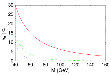
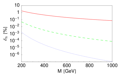
Figure 1: Relative deviations $\delta_{n}$ for low (upper panel) and high values (lower panel) of $M$. The solid, dashed, and dotted curve correspond to $n=1,2,$ and $3$, respectively. In obtaining the numerical values we have set $M_{\scriptscriptstyle Z}=91\,{\rm GeV}$ and $m_{t}=165\,{\rm GeV}$. See text for details.

Observe that there is a notable difference between the small momentum expansion and the heavy top quark mass limit. In the former case one assumes $q^{2}\ll M_{\scriptscriptstyle W}^{2},m_{t}^{2}$ while in the latter case one has $q^{2},M_{\scriptscriptstyle W}^{2}\ll m_{t}^{2}$. This difference naturally affects the convergence behavior of the series expansions. While the heavy top quark mass expansion converges slowly in the case of the non-universal one-loop SM corrections to the $Zb\bar{b}$ vertex zbb , we will demonstrate that the small momentum expansion is well behaved as long as the masses of the particles propagating in the loop are not too small, i.e., in or above the hundred ${\rm GeV}$ range.

The general features of the small momentum expansion of the one-loop $Zb\bar{b}$ vertex can be nicely illustrated with the following simple but educated example. Consider the scalar integral

$$C_{0}=\frac{m_{3}^{2}}{i\pi^{2}}\int\!\frac{d^{4}l}{D_{1}D_{2}D_{3}}\,,\hskip 14.22636ptD_{i}\equiv(l+p_{i})^{2}-m_{i}^{2}\,,$$ (2)

with $p_{3}=0$. Note that we have set the space-time dimension to four since the integral is finite and assumed without loss of generality $m_{3}\neq 0$.

In the limit of vanishing bottom quark mass one has for the corresponding momenta $p^{2}_{1}=p^{2}_{2}=0$. The small momentum expansion of the scalar integral $C_{0}$ then takes the form

$$C_{0}=\sum_{n=0}^{\infty}a_{n}\left(\frac{q^{2}}{m_{3}^{2}}\right)^{n}\,,$$ (3)

with $q^{2}=(p_{1}-p_{2})^{2}=-2\hskip 0.56905ptp_{1}\!\cdot\!p_{2}$. The expansion coefficients $a_{n}$ are given by Fleischer:1994ef

$$a_{n}=\frac{(-1)^{n}}{(n+1)!}\sum_{l=0}^{n}\begin{pmatrix}n\\ l\end{pmatrix}\frac{x_{1}^{l}}{l!}\frac{\partial^{l}}{\partial x_{1}^{l}}\frac{\partial^{n}}{\partial x_{2}^{n}}g(x_{1},x_{2})\,,$$ (4)

where

$$g(x_{1},x_{2})=\frac{1}{x_{1}-x_{2}}\left(\frac{x_{1}\ln x_{1}}{1-x_{1}}-\frac{x_{2}\ln x_{2}}{1-x_{2}}\right)\,,$$ (5)

and $x_{i}\equiv m_{i}^{2}/m_{3}^{2}$. Notice that in order to properly generate the expansion coefficients $a_{n}$ one has to keep $x_{1}$ and $x_{2}$ different even in the zero or equal mass case. The corresponding limits can only be taken at the end.

In order to illustrate the convergence behavior of the small momentum expansion of the scalar integral in Eq. (3) for on-shell kinematics, we confine ourselves to the simplified case $m_{1}=m_{2}=M$ and $m_{3}=m_{t}$. We define

$$\delta_{n}\equiv a_{n}\left(\frac{M_{\scriptscriptstyle Z}^{2}}{m_{t}^{2}}\right)^{n}\left(\sum_{l=0}^{n-1}a_{l}\left(\frac{M_{\scriptscriptstyle Z}^{2}}{m_{t}^{2}}\right)^{l}\right)^{-1}\,,$$ (6)

for $n=1,2,\ldots\,$. The $M$-dependence of the relative deviations $\delta_{n}$ is displayed in Fig. 1. We see that while for values of $M$ much below $m_{t}$ higher order terms in the small momentum expansion have to be included in order to approximate the exact on-shell result accurately, in the case of $M$ larger than $m_{t}$ already the first correction is small and higher order terms are negligible. For the two reference scales $M=80\,{\rm GeV}$ and $M=250\,{\rm GeV}$ one finds for the first three relative deviations $\delta_{n}$ numerically $+9.3\%$, $+1.4\%$, and $+0.3\%$, and $+1.1\%$, $+0.02\%$, $+0.00004\%$, respectively.

It should be clear that the two reference points $M=80\,{\rm GeV}$ and $M=250\,{\rm GeV}$ have been picked for a reason. While the former describes the situation in the SM, i.e., the exchange of two pseudo Goldstone bosons and a top quark in the loop, the latter presents a possible NP contribution arising from diagrams containing two heavy scalar fields and a top quark. The above example indicates that the differences between the values of the non-universal $Zb\bar{b}$ vertex form factors evaluated on-shell and at zero external momenta are in general much less pronounced in models with extra heavy degrees of freedom than in the SM. In view of the fact that this difference amounts to a modest effect of around $-30\%$ in the SM zbb , it is suggestive to assume that the scaling of NP contributions to the non-universal parts of the $Zb\bar{b}$ vertex is in general below the $\pm 10\%$ level. This model-independent conclusion is well supported by the explicit calculations of the one-loop corrections to the specific LH contribution to the anomalous $Zb\bar{b}$ coupling in the CMFV versions of the THDM, the MSSM, the mUED, and the LHT model presented in the next section.

We would like to stress that our general argument does not depend on the chirality of possible new interactions as it is solely based on the good convergence properties of the small momentum expansion of the relevant vertex form factors. Thus we expect it to hold in the case of RH operators as well. Notice that the assumption of MFV does not play any role in the flow of the argument itself as it is exerted only at the very end in order to establish a connection between the $Zb\bar{b}$ and $Zd_{j}\bar{d_{i}}$ vertices evaluated at zero external momenta by a proper replacement of CKM factors. Therefore it does not seem digressive to anticipate similar correlations between the flavor diagonal and off-diagonal $Z$-penguin amplitudes in many beyond-MFV scenarios in which the modification of the flavor structure is known to be dominantly non-universal, i.e., connected to the third generation. See thirdgeneration for a selection of theoretically well-motivated realizations. These issues warrant a detailed study.

III Model calculations

The above considerations can be corroborated in another, yet model-dependent way by calculating explicitly the difference between the value of the LH $Zd_{j}\bar{d_{i}}$ vertex form factor evaluated on-shell and at zero external momenta. In the following this will be done in four of the most popular, consistent, and phenomenologically viable scenarios of CMFV, i.e., the THDM, the MSSM, both for small $\tan\beta$, the mUED, and the LHT model, the latter in the case of degenerate mirror fermions. All computations have been performed in the on-shell scheme employing the ’t Hooft-Feynman gauge. The actual calculations were done with the help of the packages FeynArts Hahn:2000kx and FeynCalc Mertig:1990an , and LoopTools Hahn:1998yk and FF vanOldenborgh:1990yc for numerical evaluation.

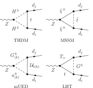
Figure 2: Examples of one-loop vertex diagrams that result in a non-universal correction to the $Z\to d_{j}\bar{d}_{i}$ transition in assorted NP scenarios with CMFV. See text for details.

Before presenting our results we collect a couple of definitions to set up our notation. In the limit of vanishing bottom quark mass, possible non-universal NP contributions to the renormalized LH off-shell $Zd_{j}\bar{d_{i}}$ vertex can be written as

$$\Gamma_{ji}^{\rm NP}=\frac{G_{F}}{\sqrt{2}}\frac{e}{\pi^{2}}M_{\scriptscriptstyle Z}^{2}\frac{c_{\scriptscriptstyle W}}{s_{\scriptscriptstyle W}}V_{tj}^{\ast}V_{ti}C_{\rm NP}(q^{2})\bar{d_{j}}_{\scalebox{0.6}{$L$}}\gamma_{\mu}{d_{i}}_{\scalebox{0.6}{$L$}}Z^{\mu}\,,$$ (7)

where $i=j=b$ and $i\neq j$ in the flavor diagonal and off-diagonal cases. $G_{F}$, $e$, $s_{\scriptscriptstyle W}$, and $c_{\scriptscriptstyle W}$ denote the Fermi constant, the electromagnetic coupling constant, the sine and cosine of the weak mixing angle, respectively, while $V_{ij}$ are the corresponding CKM matrix elements and the subscript $L$ indicates that the interactions involve LH down-type quark fields only.

As a measure of the relative difference between the complex valued form factor $C_{\rm NP}(q^{2})$ evaluated on-shell and at zero momentum we introduce

$$\delta C_{\rm NP}\equiv 1-\frac{{\rm Re}\,C_{\rm NP}(q^{2}=0)}{{\rm Re}\,C_{\rm NP}(q^{2}=M_{\scriptscriptstyle Z}^{2})}\,.$$ (8)

In the THDM with vanishing tree-level FCNCs, the only additional contribution to the $Z\to d_{j}\bar{d}_{i}$ transitions with respect to the SM comes from loops containing charged Higgs bosons, $H^{\pm}$, and top quarks, $t$. An example of such a contribution is shown on the top left-hand side of Fig. 2. The correction depends on the mass of the charged Higgs boson, $M_{H}^{\pm}$, and on the ratio of the vacuum expectation value of the Higgs doublets, $\tan\beta$. Models of type I and II differ in the way quarks couple to the Higgs doublets: in the type I scenario both the masses of down- and up-type quarks are generated by one of the doublets, like in the SM, while in the type II theory one of the doublets generates the down-type and the second one generates the up-type masses, like in the MSSM. In our case only the coupling to the top quark is relevant, so that we do not need to actually distinguish between types I and II.

To find $\delta C_{\rm THDM}$ we have computed analytically the one-loop charged Higgs corrections to Eq. (7) reproducing the result of Denner:1991ie . The analytic expression for $C_{\rm THDM}(q^{2})$ can be found in Eq. (A). The dependence of $\delta C_{\rm TDHM}$ on $M_{H}^{\pm}$ can be seen in the first panel of Fig. 3. The red (gray) band underlying the solid black curve shows the part of the parameter space satisfying the lower bound $M_{H}^{\pm}\gtrsim 295\,{\rm GeV}$ following from $\bar{B}\to X_{s}\gamma$ in the THDM of type II using the most recent SM prediction bsg . This $\tan\beta$ independent bound is much stronger than the one from the direct searches at LEP corresponding to $M_{H}^{\pm}>78.6\,{\rm GeV}$ Yao:2006px , and than the indirect lower limits from a number of other processes. In model I, the most important constraint on $M_{H}^{\pm}$ comes from $R_{b}^{0}$ Haber:1999zh . As the corresponding bound depends strongly on $\tan\beta$ we do not include it in the plot. While the decoupling of $\delta C_{\rm THDM}$ occurs slowly, we find that the maximal allowed relative suppression of ${\rm Re}\,C_{\rm THDM}(q^{2}=M_{\scriptscriptstyle Z}^{2})$ with respect to ${\rm Re}\,C_{\rm THDM}(q^{2}=0)$ is below $2\%$ and independent of $\tan\beta$, as the latter dependence exactly cancels out in Eq. (8). In obtaining the numerical values for $\delta C_{\rm TDHM}$ we have employed $M_{\scriptscriptstyle W}=80\,{\rm GeV}$, $M_{\scriptscriptstyle Z}=91\,{\rm GeV}$, $m_{t}=165\,{\rm GeV}$, and $s^{2}_{\scriptscriptstyle W}=0.23$. If not stated otherwise, the same numerical values will be used in the remainder of this article. We assess the smallness of $\delta C_{\rm THDM}$ as a first clear evidence for the correctness of our general considerations.

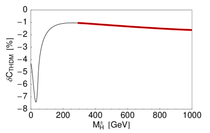
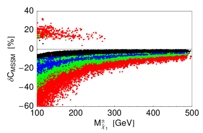
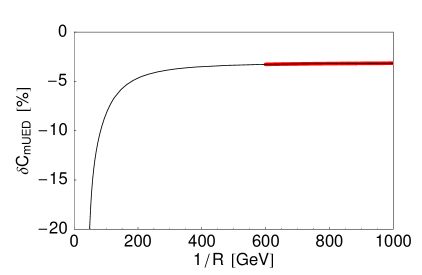
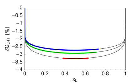
Figure 3: Relative difference $\delta C_{\rm NP}$ in the THDM, the MSSM, the mUED, and the LHT model as a function of $M_{H}^{\pm}$, $M_{\tilde{\chi}_{1}}^{\pm}$, $1/R$, and $x_{L}$. The allowed parameter regions after applying experimental and theoretical constraints are indicated by the colored (grayish) bands and points. See text for details.

In the case of the MSSM with conserved $R$-parity, we focus on the most general realization of MFV compatible with renormalization group (RG) invariance D'Ambrosio:2002ex . In this scenario CKM-type flavor- and $CP$-violating terms appear necessarily in the down- and up-type squark mass-squared matrices due to the symmetry principle underlying the MFV hypothesis. The explicit form of the physical up-type squark mass matrix used in our analysis is given in Eq. (27). We assume universality of soft supersymmetry (SUSY) breaking masses and proportionality of trilinear terms at the EW scale, so that neutralino and gluino contributions to flavor-changing $Z\to d_{j}\bar{d}_{i}$ transitions are absent. This additional assumption about the structure of the soft breaking terms in the squark sector has a negligible effect on the considered FCNC processes Isidori:2006qy . Moreover, in the small $\tan\beta$ regime both neutralino and neutral Higgs corrections to $Z\to b\bar{b}$ turn out to be insignificant Boulware:1991vp . Therefore only SUSY diagrams involving chargino, $\tilde{\chi}^{\pm}$, and stop, $\tilde{t}$, exchange are relevant here. An example of such a contribution can be seen on the top right side of Fig. 2. A noticeable feature in the chosen setting is that large left-right mixing can occur in the stop sector, leading to both a relatively heavy Higgs in the range $120\,{\rm GeV}\lesssim M_{h}^{0}\lesssim 135\,{\rm GeV}$ and a stop mass eigenstate, say, $\tilde{t}_{1}$, possibly much lighter than the remaining squarks. Such a scenario corresponds to the “golden region” of the MSSM, where all experimental constraints are satisfied and fine-tuning is minimized Perelstein:2007nx . For what concerns the other sfermions we neglect left-right mixing and assume that all squarks and sleptons have a common mass $m_{\tilde{q}}$ and $m_{\tilde{l}}$, respectively.

In order to find the complete MSSM correction $\delta C_{\rm MSSM}$ we have calculated analytically the one-loop chargino-up-squark corrections to Eq. (7) and combined it with the charged Higgs contribution. Our result for $C_{\tilde{\chi}^{\pm}}(q^{2})$ agrees with the one of Boulware:1991vp and is given in Eq. (A). The region of parameters in which the SUSY corrections to the LH $Zd_{j}\bar{d_{i}}$ vertices are maximal corresponds to the case of a light stop and chargino. In our numerical analysis we therefore focus on these scenarios. We allow the relevant MSSM parameters to float freely in the ranges $2<\tan\beta<6$, $|\mu|<500\,{\rm GeV}$, and $M<1\,{\rm TeV}$ for $M=M_{H}^{\pm},M_{2},m_{\tilde{t}_{1}},m_{\tilde{q}},m_{\tilde{l}}$. The value of the trilinear coupling $A_{u}$ is computed from each randomly chosen set of parameters $\mu$, $m_{\tilde{t}_{1}}$, and $m_{\tilde{q}}$. The calculation of $b\to s\gamma$ and $b\to sl^{+}l^{-}$ that is used to constrain the parameter space introduces also a dependence on the gluino mass $M_{\tilde{g}}$. We choose to vary $M_{\tilde{g}}$ in the range $241\,{\rm GeV}<M_{\tilde{g}}<1\,{\rm TeV}$ Abazov:2006bj .

The MSSM parameter space is subject to severe experimental and theoretical constraints. We take into account the following lower bounds on the particle masses Yao:2006px : $M_{H}^{\pm}>78.6\,{\rm GeV}$, $M_{\tilde{\chi}_{1}}^{\pm}>94\,{\rm GeV}$, $m_{\tilde{t}_{1}}>95.7\,{\rm GeV}$, $m_{\tilde{q}}>99.5\,{\rm GeV}$, and $m_{\tilde{l}}>73\,{\rm GeV}$. In the considered parameter space the requirement of the absence of color and/or charge breaking minima sets a strong upper limit of around $3\,{\rm TeV}$ on the absolute value of $A_{u}$ ccbreak . As far as the lightest neutral Higgs boson is concerned, we ensure that $M_{h}^{0}>114.4\,{\rm GeV}$ ewpm , including the dominant radiative corrections mhsusy to its tree-level mass. Further restrictions that we impose on the SUSY parameter space are the $\rho$ parameter rhosusy , $R_{b}^{0}$ Boulware:1991vp , and the inclusive $b\to s\gamma$ bsgsusy and $b\to sl^{+}l^{-}$ Bobeth:2004jz branching fractions. To find the boundaries of the allowed parameter space we perform an adaptive scan of the eight SUSY variables employing the method advocated in adaptive .

The dependence of $\delta C_{\rm MSSM}$ on the lighter chargino mass $M_{\tilde{\chi}_{1}}^{\pm}$ is illustrated in the second plot of Fig. 3. Regions in the $M_{\tilde{\chi}_{1}}^{\pm}$–$\,\delta C_{\rm MSSM}$ plane where the absolute value of the correction ${\rm Re}\,C_{\rm MSSM}(q^{2}=0)$ amounts to at least $2\%$, $4\%$, $6\%$, and $10\%$ of the SM value ${\rm Re}\,C_{\rm SM}(q^{2}=0)$ are indicated by the red (gray), green (light gray), blue (dark gray), and black points, respectively. No constraints are imposed for the black points while the colored (grayish) ones pass all the collider and low-energy constraints mentioned above.

Three features of our numerical explorations deserve special mention. First, the maximal allowed relative size of the correction ${\rm Re}\,C_{\rm MSSM}(q^{2}=0)$ amounts to less than ${}^{+9\%}_{-6\%}$ of ${\rm Re}\,C_{\rm SM}(q^{2}=0)$. Second, the magnitude of the possible deviation $\delta C_{\rm MSSM}$ is strongly anti-correlated with the absolute size of ${\rm Re}\,C_{\rm MSSM}(q^{2}=0)$. While small corrections ${\rm Re}\,C_{\rm MSSM}(q^{2}=0)$ allow for large values of $\delta C_{\rm MSSM}$ the latter difference decreases rapidly with increasing ${\rm Re}\,C_{\rm MSSM}(q^{2}=0)$. Third, the correction $\delta C_{\rm MSSM}$ decouples quickly for heavy charginos. These features imply that $\delta C_{\rm MSSM}$ is small if one requires $(i)$ the relative size of ${\rm Re}\,C_{\rm MSSM}(q^{2}=0)$ to be observable, i.e., to be bigger than the SM uncertainty of the universal $Z$-penguin function and $(ii)$ the chargino mass $M_{\tilde{\chi}_{1}}^{\pm}$ to be not too light. For example, all allowed points satisfy $|\delta C_{\rm MSSM}|<0.01$ if one demands $|{\rm Re}\,C_{\rm MSSM}(q^{2}=0)/{\rm Re}\,C_{\rm SM}(q^{2}=0)|>0.05$ and $M_{\tilde{\chi}_{1}}^{\pm}>300\ {\rm GeV}$. On the other hand, if the masses of the lighter chargino and stop both lie in the hundred ${\rm GeV}$ range, $\delta C_{\rm MSSM}$ frequently turns out to be larger than one would expected on the basis of our model-independent considerations.

The large corrections $\delta C_{\rm MSSM}$ can be traced back to the peculiar structure of the form factor $C_{\tilde{\chi}^{\pm}}(q^{2})$. While in the limit of vanishing external $Z$-boson momentum the first three terms in Eq. (A) all approach a constant value the fourth one scales like $q^{2}/M_{\rm SUSY}^{2}$ with $M_{\rm SUSY}={\rm min}(M_{\tilde{\chi}_{1}}^{\pm},m_{\tilde{t}_{1}})$. Naively, one thus would expect the general argument given in the last section to hold. Yet for large left-right mixing in the stop sector, which permits a relatively heavy Higgs mass of $M_{h}^{0}\gtrsim 120\,{\rm GeV}$, it turns out that the first three contributions tend to cancel each other and, in turn, the size of $\delta C_{\rm MSSM}$ is controlled by the fourth term. Then $\delta C_{\rm MSSM}\propto M_{\scriptscriptstyle Z}^{2}/M_{\rm SUSY}^{2}$ and the correction $\delta C_{\rm MSSM}$ can be sizable if $M_{\rm SUSY}$ is close to the EW scale. The observed numerical cancellation also explains why $\delta C_{\rm MSSM}$ is typically large if ${\rm Re}\,C_{\rm MSSM}(q^{2}=0)$ is small and vice versa. It should be clear, however, that the large deviation $\delta C_{\rm MSSM}$ are ultimately no cause of concern, because $|{\rm Re}\,C_{\rm MSSM}(q^{2}=0)/{\rm Re}\,C_{\rm SM}(q^{2}=0)|$ itself is always below $10\%$. In consequence, the model-independent bound on the NP contribution to the universal $Z$-penguin function that we will derive in the next section does hold in the case of the CMFV MSSM.

Among the most popular non-SUSY models in question is the model of Appelquist, Cheng, and Dobrescu (ACD) Appelquist:2000nn . In the ACD framework the SM is extended from four-dimensional Minkowski space-time to five dimensions and the extra space dimension is compactified on the orbifold $S^{1}/Z_{2}$ in order to obtain chiral fermions in four dimensions. The five-dimensional fields can equivalently be described in a four-dimensional Lagrangian with heavy Kaluza-Klein (KK) states for every field that lives in the fifth dimension or bulk. In the ACD model all SM fields are promoted to the bulk and in order to avoid large FCNCs tree-level boundary fields and interactions are assumed to vanish at the cut-off scale. A remnant of the translational symmetry after compactification leads to KK-parity. This property implies, that KK states can only be pair-produced, that their virtual effect comes only from loops, and causes the lightest KK particle to be stable, therefore providing a viable dark matter candidate ueddm .

In the following we will assume vanishing boundary terms at the cut-off scale and that the ultraviolet (UV) completion does not introduce additional sources of flavor and $CP$ violation beyond the ones already present in the model. These additional assumptions define the mUED model which then belongs to the class of CMFV scenarios. The one-loop correction to $\Gamma_{ji}^{\rm mUED}$ is found from diagrams containing apart from the ordinary SM fields, infinite towers of the KK modes corresponding to the $W$-boson, $W^{\pm}_{(k)}$, the pseudo Goldstone boson, $G^{\pm}_{(k)}$, the $SU(2)$ quark doublets, ${\cal Q}_{q(k)}$, and the $SU(2)$ quark singlets, ${\cal U}_{q(k)}$. Additionally, there appears a charged scalar, $a^{\pm}_{(k)}$, which has no counterpart in the SM. A possible diagram involving such a KK excitation is shown on the lower left side in Fig. 2. Since at leading order the $Z\to d_{j}\bar{d}_{i}$ amplitude turns out to be cut-off independent the only additional parameter entering $\Gamma_{ji}^{\rm mUED}$ relative to the SM is the inverse of the compactification radius $1/R$. The analytic expression for $C_{\rm mUED}(q^{2})$ can be found in Eq. (A).

For a light Higgs mass of $M_{h}^{0}=115\,{\rm GeV}$ a careful analysis of oblique corrections Gogoladze:2006br gives a lower bound of $1/R\gtrsim 600\,{\rm GeV}$, well above current collider limits acdcollider . With increasing Higgs mass this constraint relaxes significantly leading to $1/R\gtrsim 300\,{\rm GeV}$ Gogoladze:2006br ; Appelquist:2002wb . Other constraints on $1/R$ that derive from $R_{b}^{0}$ Oliver:2002up , the muon anomalous magnetic moment Appelquist:2001jz , and flavor observables Buras:2002ej ; Buras:2003mk ; acdflavor are in general weaker. An exception is the inclusive $\bar{B}\to X_{s}\gamma$ branching ratio. Since the SM prediction bsg is now lower than the experimental world average by more than $1\hskip 1.13809pt\sigma$ and the one-loop KK contributions interfere destructively with the SM $b\to s\gamma$ amplitude Buras:2003mk ; Agashe:2001xt , $\bar{B}\to X_{s}\gamma$ provides at leading order the lower bound $1/R\gtrsim 600\,{\rm GeV}$ independent from the Higgs mass Haisch:2007vb . The $1/R$ dependence of $\delta C_{\rm mUED}$ is displayed in the third plot of Fig. 3. In the range of allowed compactification scales, indicated by the red (gray) stripe, the suppression of ${\rm Re}\,C_{\rm mUED}(q^{2}=M_{\scriptscriptstyle Z}^{2})$ compared to ${\rm Re}\,C_{\rm mUED}(q^{2}=0)$ amounts to less than $5\%$, the exact value being almost independent of $1/R$. This lends further support to the conclusion drawn in the last section. We finally note that our new result for $C_{\rm mUED}(q^{2})$ coincides for $q^{2}=0$ with the one-loop KK contribution to the $Z$-penguin function calculated in Buras:2002ej .

Another phenomenologically very promising NP scenario is the LHT model. Here the Higgs is a pseudo Goldstone boson arising from the spontaneous breaking of an approximate global $SU(5)$ symmetry down to $SO(5)$ Arkani-Hamed:2002qy at a scale $f$. To make the existence of new particle in the $1\,{\rm TeV}$ range consistent with precision EW data, an additional discrete $Z_{2}$ symmetry called $T$-parity tparity , is introduced, which as one characteristic forbids tree-level couplings that violate custodial $SU(2)$ symmetry. In the fermionic sector, bounds on four fermion operators demand for a consistent implementation of this reflection symmetry the existence of a copy of all SM fermions, aptly dubbed mirror fermions Low:2004xc . The theoretical concept of $T$-parity and its experimental implications resemble the one of $R$-parity in SUSY and KK-parity in universal extra dimensional theories.

Unless their masses are exactly degenerate, the presence of mirror quarks leads in general to new flavor- and $CP$-violating interactions. In order to maintain CMFV we are thus forced to assume such a degeneracy here. In this case contributions from particles that are odd under $T$-parity vanish due to the Glashow-Iliopoulos-Maiani (GIM) mechanism Glashow:1970gm , and the only new particle that affects the $Z\to d_{j}\bar{d}_{i}$ transition in a non-universal way is a $T$-even heavy top, $T_{+}$. A sample diagram involving such a heavy top, its also $T$-even partner, i.e., the top quark $t$, and a pseudo Goldstone field, $G^{\pm}$, is shown on the lower right-hand side of Fig. 2. In turn, $\Gamma_{ji}^{\rm LHT}$ depends only on the mass of the heavy quark $T_{+}$, which is controlled by the size of the top Yukawa coupling, by $f$, and the dimensionless parameter $x_{L}\equiv\lambda_{1}^{2}/(\lambda_{1}^{2}+\lambda_{2}^{2})$. Here $\lambda_{1}$ is the Yukawa coupling between $t$ and $T_{+}$ and $\lambda_{2}$ parametrizes the mass term of $T_{+}$. In the fourth panel of Fig. 3, we show from bottom to top $\delta C_{\rm LHT}$ as a function of $x_{L}$ for $f=1,1.5,$ and $2\,{\rm TeV}$. The colored (grayish) bands underlying the solid black curves correspond to the allowed regions in parameter space after applying the constraints following from precision EW data Hubisz:2005tx . As NP effects in the quark flavor sector of the LHT model with CMFV are generically small lhtflavor ; Blanke:2006eb , they essentially do not lead to any restrictions. We find that the maximal allowed suppression of ${\rm Re}\,C_{\rm LHT}(q^{2}=M_{\scriptscriptstyle Z}^{2})$ with respect to ${\rm Re}\,C_{\rm LHT}(q^{2}=0)$ is slightly bigger than $3\%$. This feature again confirms our general considerations. Our new result for $C_{\rm LHT}(q^{2})$ given in Eq. (A) resembles for $q^{2}=0$ the analytic expression of the one-loop correction to the low-energy $Z$-penguin function calculated in Blanke:2006eb . Taking into account that the latter result corresponds to unitary gauge while we work in ’t Hooft-Feynman gauge is essential for this comparison. In particular, in our case no UV divergences remain after GIM, as expected on general grounds Bardeen:2006wk .

At this point a further comment concerning gauge invariance is in order. It is well known that only a proper arrangement of, say, $e^{+}e^{-}\to f\bar{f}$, including all contributions related to the $Z$-boson, purely EW boxes, and the photon, is gauge invariant at a given order in perturbation theory. In flavor physics such a gauge independent decomposition Buchalla:1990qz is provided by the combinations $X\equiv C+B^{\nu\bar{\nu}}$, $Y\equiv C+B^{l^{+}l^{-}}$, and $Z\equiv C+D/4$ of Inami-Lim functions Inami:1980fz . Given the normalization of Eq. (7), NP contributions to the universal $Z$-penguin function $C$ are characterized by ${\rm Re}\,C_{\rm NP}(q^{2}=0)$ in our notation, while $B^{\nu\bar{\nu}}$ and $B^{l^{+}l^{-}}$ represent the contribution of EW boxes with neutrino and charged lepton pairs in the final state. $D$ stems from the off-shell part of the magnetic photon penguin amplitude. Since we want to relate in a model-independent way observables derived from $e^{+}e^{-}\to f\bar{f}$ to observables connected with the $d_{i}\to d_{j}\nu\bar{\nu}$ and $d_{i}\to d_{j}l^{+}l^{-}$ transitions, we also have to worry about the potential size of corrections that are not associated with the $Z$-boson.

At the $Z$-pole, the total cross-section of $e^{+}e^{-}\to f\bar{f}$ is completely dominated by $Z$-boson exchange. While purely EW boxes are vanishingly small, the bulk of the radiative corrections necessary to interpret the measurements are QED effects. It is important to realize that these QED corrections are essentially independent of the EW ones, and therefore allow the anomalous $Zb\bar{b}$ couplings to be extracted from the data in a model-independent manner. Certain SM assumptions are nevertheless employed when extracting and interpreting the couplings, but considerable effort ewpm has been expended to make the extraction of the POs $R_{b}^{0}$, ${\cal A}_{b}$, and $A_{\rm FB}^{0,b}$ as model-independent as possible, so that the meanings of theory and experiment remain distinct.

In the case of the $d_{i}\to d_{j}\nu\bar{\nu}$ and $d_{i}\to d_{j}l^{+}l^{-}$ observables theoretical assumptions about the size of the EW boxes are unfortunately indispensable. Our explicit analysis of the considered CMFV models reveals the following picture. In the THDM, the NP contributions $\Delta B^{\nu\bar{\nu}}\equiv B^{\nu\bar{\nu}}-B^{\nu\bar{\nu}}_{\rm SM}$ and $\Delta B^{l^{+}l^{-}}\equiv B^{l^{+}l^{-}}-B^{l^{+}l^{-}}_{\rm SM}$ vanish identical Bobeth:2001jm , while their relative sizes compared to the corresponding SM contributions amount to at most ${}^{+1}_{-11}\%$ and ${}^{+18}_{-5}\%$ in the MSSM Buras:2000qz and less than $+1\%$ in both the mUED scenario Buras:2002ej and the LHT model Blanke:2006eb . The numbers for $\Delta B^{\nu\bar{\nu}}$, $\Delta B^{l^{+}l^{-}}$, and $\Delta C$ quoted here and in the following refer to the ’t Hooft-Feynman gauge. Moreover, contributions to the EW boxes are found to be generically suppressed by at least two inverse powers of the scale of NP using naive dimensional analysis Buras:1999da . In view of this, the possibility of substantial CMFV contributions to the EW boxes seems rather unlikely. The actual size of the NP contribution $\Delta D\equiv D-D_{\rm SM}$ to the off-shell magnetic photon penguin function $D$ has essentially no impact on our conclusions. The treatment of $\Delta B^{\nu\bar{\nu}}$, $\Delta B^{l^{+}l^{-}}$, and $\Delta D$ in our numerical analysis will be discussed in the next section.

IV Numerical analysis

Our numerical analysis consists of three steps. First we determine the CKM parameters $\bar{\rho}$ and $\bar{\eta}$ from an analysis of the universal UT Buras:2000dm . The actual analysis is performed with a customized version of the CKMfitter package Charles:2004jd . Using the numerical values of the experimental and theoretical parameters collected in App. B we find

$$\bar{\rho}=0.160\pm 0.031\,,\hskip 14.22636pt\bar{\eta}=0.326\pm 0.012\,.$$ (9)

The given central values are highly independent of $m_{t}$, but depend mildly on the hadronic parameter $\xi\equiv(f_{B_{s}}\hat{B}_{B_{s}}^{1/2})/(f_{B_{d}}\hat{B}_{B_{d}}^{1/2})$ determined in lattice QCD. Since in our approach theoretical parameter ranges are scanned, the quoted $68\%$ confidence levels (${\rm CL}$s) should be understood as lower bounds, i.e., the range in which the quantity in question lies with a probability of at least $68\%$. The same applies to all ${\rm CL}$s and probability regions given subsequently.

In the second step, we determine the allowed ranges of $\Delta C$ and the NP contribution $\Delta C_{7}^{\rm eff}\equiv C_{7}^{\rm eff}(m_{b})-C_{7\,{\rm SM}}^{\rm eff}(m_{b})$ to the effective on-shell magnetic photon penguin function from a careful combination of the results of the POs $R_{b}^{0}$, ${\cal A}_{b}$, and $A_{\rm FB}^{0,b}$ ewpm with the measurements of the branching ratios of $\bar{B}\to X_{s}\gamma$ bsgamma and $\bar{B}\to X_{s}l^{+}l^{-}$ bxsll . In contrast to Bobeth:2005ck , we do not include the available experimental information on $K^{+}\to\pi^{+}\nu\bar{\nu}$ kp in our global fit, as the constraining power of the latter measurement depends in a non-negligible way on how the experimental ${\rm CL}$ of the signal kpcl is implemented in the analysis.

Third, and finally, we use the derived ranges for the Inami-Lim functions in question to find lower and upper bounds for the branching ratios of the rare decays $K^{+}\to\pi^{+}\nu\bar{\nu}$, $K_{L}\to\pi^{0}\nu\bar{\nu}$, $K_{L}\to\mu^{+}\mu^{-}$, $\bar{B}\to X_{d,s}\nu\bar{\nu}$, and $B_{d,s}\to\mu^{+}\mu^{-}$ within CMFV.

Our data set includes all POs measured at LEP and SLC that are related to the $Z\to b\bar{b}$ decay. It is given in Tab. 1. Concerning the used data we recall that the ratio $4/3\,A_{\rm FB}^{0,b}/{\cal A}_{e}$ is lower than the direct measurement of ${\cal A}_{b}$ by $1.6\hskip 1.13809pt\sigma$, and lower than the SM expectation for ${\cal A}_{b}$ by $3.2\hskip 1.13809pt\sigma$ ewpm . Whether this is an experimental problem, an extreme statistical fluctuation or a real NP effect in the bottom quark couplings is up to date unresolved. In fact, the relative experimental error in $A_{\rm FB}^{0,b}$ is much larger than the ones in the total $Z\to b\bar{b}$ rate, $R_{b}^{0}$, and ${\cal A}_{b}$, where no anomalies are observed. Furthermore, the extracted value of the anomalous LH coupling of the bottom quark agrees with its SM value because of the strong constraint given by $R_{b}^{0}$. This strong constraint carries over to our results, which do not depend notably on whether $A_{\rm FB}^{0,b}$ is included in or excluded from the data set. We assume that statistical fluctuations are responsible for the observed discrepancy and include $A_{\rm FB}^{0,b}$ in our global fit.

The actual calculations of $R_{b}^{0}$, ${\cal A}_{b}$, and $A_{\rm FB}^{0,b}$ used in our analysis are performed with ZFITTER zfitter , which includes the SM purely EW, QED and QCD radiative effects, photon exchange and $\gamma$-$Z$ interference that are necessary to extract the POs in a model-independent manner. For the purpose of our analysis, ZFITTER has been modified to include possible NP contributions to the $Zb\bar{b}$ vertex in the parametrization of Eq. (7). The Higgs mass is allowed to vary freely in the range $100\,{\rm GeV}<M_{h}^{0}<600\,{\rm GeV}$. Since $R_{b}^{0}$ is largely insensitive to the mass of the Higgs boson this conservative range has no noticeable impact on our results. The input values of the other parameters entering $R_{b}^{0}$, ${\cal A}_{b}$, and $A_{\rm FB}^{0,b}$ are collected in App. B.

Table 1: Results and correlations for the $Z\to b\bar{b}$ POs of the fit to the LEP and SLC heavy flavor data taken from ewpm .

Observable	Result	$R_{b}^{0}$	${\cal A}_{b}$	$A_{\rm FB}^{0,b}$
$R_{b}^{0}$	$0.21629\pm 0.00066$	$1.00$	$-0.08$	$-0.10$
${\cal A}_{b}$	$0.923\pm 0.020$		$\phantom{+}1.00$	$\phantom{+}0.06$
$A_{\rm FB}^{0,b}$	$0.0992\pm 0.0016$			$\phantom{+}1.00$

The experimental results that we consider in connection with $\bar{B}\to X_{s}\gamma$ and $\bar{B}\to X_{s}l^{+}l^{-}$ are summarized in Tab. 2. The given weighted average of the branching ratio ${\cal B}(\bar{B}\to X_{s}\gamma)$ corresponds to a photon energy cut $E_{\gamma}>1.6\,{\rm GeV}$ in the $\bar{B}$-meson rest frame, while for ${\cal B}(\bar{B}\to X_{s}l^{+}l^{-})$ the experimental data in the low-$q^{2}$ region $1\,{\rm GeV}^{2}<q^{2}<6\,{\rm GeV}^{2}$ of the dilepton invariant mass squared, averaged over electrons and muons are shown. Our calculations rely on bsg in the case of $\bar{B}\to X_{s}\gamma$ and on bsll in the case of $\bar{B}\to X_{s}l^{+}l^{-}$. The used numerical input parameters can be found in App. B. Unlike Bobeth:2005ck , we do not include $\bar{B}\to X_{s}l^{+}l^{-}$ data on the regions $0.04\,{\rm GeV}^{2}<q^{2}<1\,{\rm GeV}^{2}$ and $14.4\,{\rm GeV}^{2}<q^{2}<25\,{\rm GeV}^{2}$ in our analysis. The reason for this omission is twofold. First, in these regions the differential $\bar{B}\to X_{s}l^{+}l^{-}$ rate is less sensitive to $\Delta C$ than in the low-$q^{2}$ region. Second, for high $q^{2}$ the theoretical uncertainties are larger with respect to the ones that affect the low-$q^{2}$ region. An inclusion of the latter two constraints would therefore make the fit more complicated, but it would not improve the quality of the obtained results.

Table 2: World averages of ${\cal B}(\bar{B}\to X_{s}\gamma)$ for $E_{\gamma}>1.6\,{\rm GeV}$ and ${\cal B}(\bar{B}\to X_{s}l^{+}l^{-})$ for $1\,{\rm GeV}^{2}<q^{2}<6\,{\rm GeV}^{2}$.

Observable	Result
${\cal B}(\bar{B}\to X_{s}\gamma)\times 10^{4}$	$3.55\pm 0.26$  Barbiero:2007cr
${\cal B}(\bar{B}\to X_{s}l^{+}l^{-})\times 10^{6}$	$1.60\pm 0.51$  bxsll

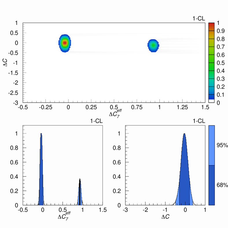
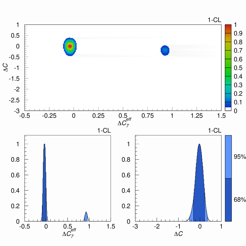
Figure 4: The upper (lower) panel displays the constraints on $\Delta C_{7}^{\rm eff}$ and $\Delta C$ within CMFV scanning $\Delta B^{l^{+}l^{-}}$ in the range $\pm 0.1$ (set to zero) that follow from a combination of the $Z\to b\bar{b}$ POs with flavor observables. The colors encode the frequentist $1-{\rm CL}$ level and the corresponding $68\%$ and $95\%$ probability regions as indicated by the bars on the right side of the panels. See text for details.

Before we present our final results, additional comments on the used methodology concerning $\Delta B^{\nu\bar{\nu}}$, $\Delta B^{l^{+}l^{-}}$, $\Delta C$, $\Delta D$, and $\Delta C_{7}^{\rm eff}$ are in order. We begin with $\Delta C_{7}^{\rm eff}$ which enters both $\bar{B}\to X_{s}\gamma$ and $\bar{B}\to X_{s}l^{+}l^{-}$. A well-known way to avoid the $\bar{B}\to X_{s}\gamma$ constraint consists in having a large positive NP contribution $\Delta C_{7}^{\rm eff}$ that approximately reverses the sign of the amplitude ${\cal A}(b\to s\gamma)\propto C_{7}^{\rm eff}(m_{b})$ with respect to the SM and leaves ${\cal B}(\bar{B}\to X_{s}\gamma)\propto|C_{7}^{\rm eff}(m_{b})|^{2}$ unaltered within experimental and theoretical uncertainties. In our analysis, we add $\Delta C_{7}^{\rm eff}$ to the top quark contribution of the SM, keeping $m_{b}$ that multiplies this combination renormalized at $m_{t}$. This rescaling is motivated by the observation Gambino:2001ew , that in this way most of the logarithmic enhanced QCD corrections are properly taken into account. We recall that $C_{7\,{\rm SM}}^{\rm eff}(m_{b})\simeq-0.38$ in this approach.

Both the value and the sign of $C_{7}^{\rm eff}(m_{b})$ play an important role in the $\bar{B}\to X_{s}l^{+}l^{-}$ decay rate wcbsll . By contrast the dependence of ${\cal B}(\bar{B}\to X_{s}l^{+}l^{-})$ on $D$ is relatively weak. Nevertheless, for suitable chosen values of $\Delta D$ the $\bar{B}\to X_{s}l^{+}l^{-}$ constraint can be always satisfied even in the case of the non-SM solution of $\Delta C_{7}^{\rm eff}$. In consequence, $\Delta D$ is not well constrained by the data used, and we decided to scan $\Delta D$ in the range $\pm 1$ for the best fit value. This choice is rather generous since in the CMFV scenarios that we consider one has $|\Delta D|<|D_{\rm SM}|$ with $D_{\rm SM}\simeq-0.49$ throughout the allowed parameter space Buras:2002ej ; Blanke:2006eb ; Buras:2000qz ; dthdm . We verified that even larger variations have basically no effect on the extraction of the allowed range for $\Delta C$, since the $Z\to b\bar{b}$ POs do not depend on $\Delta D$. The impact of $\Delta D$ on the bounds of $\Delta C_{7}^{\rm eff}$ will be discussed below.

Precision data on $R_{b}^{0}$, ${\cal A}_{b}$, and $A_{\rm FB}^{0,b}$ lead to a tight, highly model-independent constraint on ${\rm Re}\,C_{\rm NP}(q^{2}=M_{\scriptscriptstyle Z}^{2})$. The allowed range of $\Delta C$ can then be calculated from the identity $\Delta C=(1+\delta C_{\rm NP}){\rm Re}\,C_{\rm NP}(q^{2}=M_{\scriptscriptstyle Z}^{2})$ in any given model of NP where $\delta C_{\rm NP}$ is known. To carry out the analysis in a generic way, one, however, needs to make an assumption about the size of $\delta C_{\rm NP}$. Guided by the results of Secs. II and III we allow $\delta C_{\rm NP}$ to float in the range $\pm 0.1$. We note that larger variations with, say, an absolute value of $|\delta C_{\rm SM}|\simeq 0.3$, still lead to the conclusion that large negative values of $\Delta C$ that would reverse the sign of $C_{\rm SM}\simeq 0.78$ are highly disfavored.

The only EW box that enters the determination of $\Delta C_{7}^{\rm eff}$ and $\Delta C$ in our case is $\Delta B^{l^{+}l^{-}}$. To explore the impact of the size of EW boxes on the fit results we consider two scenarios. In the first we allow $\Delta B^{l^{+}l^{-}}$ to vary in the range $\pm 0.1$ while in the second we assume $\Delta B^{l^{+}l^{-}}=0$. The former choice seems conservative, as relative to the SM value $B^{l^{+}l^{-}}_{\rm SM}\simeq 0.18$ possible $\Delta B^{l^{+}l^{-}}$ contributions amount to only ${}^{+18}_{-5}\%$ in the MSSM with MFV and small $\tan\beta$ Buras:2000qz and to below $+1\%$ in both the mUED Buras:2002ej and the LHT model with degenerate mirror fermions Blanke:2006eb . In fact, the actual size of $\Delta B^{l^{+}l^{-}}$, which enters our fit through ${\cal B}(\bar{B}\to X_{s}l^{+}l^{-})$, does only have a marginal effect on the results, because $C$ is already tightly constraint by the combination of $R_{b}^{0}$, ${\cal A}_{b}$, and $A_{\rm FB}^{0,b}$. Our bound on $\Delta C$ does not, for that reason, depend on any conjecture concerning the size of EW boxes. Notice that this is not the case in the analysis of the “Magnificent Seven” Bobeth:2005ck ; M7 , which relies on the assumption $\Delta B^{\nu\bar{\nu}}=\Delta B^{l^{+}l^{-}}=0$ to derive a probability distribution function for $\Delta C$.

The constraints on $\Delta C_{7}^{\rm eff}$ and $\Delta C$ within CMFV following from the simultaneous use of $R_{b}^{0}$, ${\cal A}_{b}$, $A_{\rm FB}^{0,b}$, ${\cal B}(\bar{B}\to X_{s}\gamma)$, and ${\cal B}(\bar{B}\to X_{s}l^{+}l^{-})$ can be seen in Fig. 4. All panels show frequentist $1-{\rm CL}$ levels. We see from the top and the lower left plots that two regions, resembling the two possible signs of $C_{7}^{\rm eff}(m_{b})$, satisfy all existing experimental bounds. The best fit value for $\Delta C_{7}^{\rm eff}$ is very close to the SM point residing in the origin, while the wrong-sign solution located on the right in the upper (lower) panel is barely (not) accessible at $68\%$ probability, as it corresponds to a ${\cal B}(\bar{B}\to X_{s}l^{+}l^{-})$ value considerably higher than the measurements Gambino:2004mv . In the upper (lower) panel of Fig. 4 the contribution $\Delta B^{l^{+}l^{-}}$ is scanned in the range $\pm 0.1$ (set to zero). In the former case the full results read

$$\begin{gathered}\Delta C_{7}^{\rm eff}=-0.039\pm 0.043\,\cup\,0.931\pm 0.016\;\;(68\%\,{\rm CL})\,,\hskip 8.53581pt\\ \Delta C_{7}^{\rm eff}=[-0.104,0.026]\,\cup\,[0.874,0.988]\;\;(95\%\,{\rm CL})\,,\hskip 5.69054pt\end{gathered}$$ (12)

while in the latter one we obtain

$$\begin{gathered}\Delta C_{7}^{\rm eff}=-0.039\pm 0.043\;\;(68\%\,{\rm CL})\,,\hskip 5.69054pt\\ \Delta C_{7}^{\rm eff}=[-0.104,0.026]\,\cup\,[0.890,0.968]\;\;(95\%\,{\rm CL})\,.\hskip 5.69054pt\end{gathered}$$ (15)

Similar bounds have been presented previously in Bobeth:2005ck . A comparison of Eq. (12) with Eq. (15) makes clear that the size of $\Delta B^{l^{+}l^{-}}$ has only a moderate impact on the accessibility of the non-SM solution of $\Delta C_{7}^{\rm eff}$ while it leaves the ranges themselves almost unchanged. Nevertheless, for $|\Delta B^{l^{+}l^{-}}|>|B^{l^{+}l^{-}}_{\rm SM}|$ the wrong-sign case $\Delta C_{7}^{\rm eff}\simeq 0.93$ cannot be excluded on the basis of ${\cal B}(\bar{B}\to X_{s}\gamma)$ and ${\cal B}(\bar{B}\to X_{s}l^{+}l^{-})$ measurements alone. The same statements apply to $\Delta D$ although its impact on the obtained results is less pronounced than the one of $\Delta B^{l^{+}l^{-}}$. Notice that since the SM prediction of ${\cal B}(\bar{B}\to X_{s}\gamma)$ bsg is now lower than the experimental world average by more than $1\hskip 1.13809pt\sigma$, extensions of the SM that predict a suppression of the $b\to s\gamma$ amplitude are strongly constrained. In particular, even the SM point $\Delta C_{7}^{\rm eff}=0$ is almost disfavored at $68\%\,{\rm CL}$ by the global fit. This tension is not yet significant, but could become compelling once the experimental and/or theoretical error on ${\cal B}(\bar{B}\to X_{s}\gamma)$ has been further reduced.

As can be seen from the top and the lower right plots in Fig. 4, in the case of $\Delta C$ only small deviations from the SM are compatible with the data. In the upper (lower) panel of Fig. 4 the contribution $\Delta B^{l^{+}l^{-}}$ is varied in the range $\pm 0.1$ (set to zero). In the former case we find the following bounds

$$\Delta C =-0.037\pm 0.266 \!\!(68\%\,{\rm CL})\,,$$ (16)

$$\Delta C =[-0.493,0.387] \!\!(95\%\,{\rm CL})\,,$$

while in the latter one we get

$$\Delta C =-0.026\pm 0.264 \!\!(68\%\,{\rm CL})\,,$$ (17)

$$\Delta C =[-0.483,0.368] \!\!(95\%\,{\rm CL})\,.$$

These results imply that large negative contributions to $C$ that would reverse the sign of the SM $Z$-penguin amplitude are highly disfavored in CMFV scenarios due to the strong constraint from the $Z\to b\bar{b}$ POs, most notably, the one from $R_{b}^{0}$. We stress that we could not have come to this conclusion by considering only flavor constraints, as done in Bobeth:2005ck , since at present a combination of ${\cal B}(\bar{B}\to X_{s}\gamma)$, ${\cal B}(\bar{B}\to X_{s}l^{+}l^{-})$, and ${\cal B}(K^{+}\to\pi^{+}\nu\bar{\nu})$ does not allow one to distinguish the SM solution $\Delta C=0$ from the wrong-sign case $\Delta C\approx-2$. Eqs. (16) and (17) also show that the derived bound on $\Delta C$ is largely insensitive to the size of potential EW box contributions which is not the case if the $Z\to b\bar{b}$ POs constraints are replaced by the one stemming from ${\cal B}(K^{+}\to\pi^{+}\nu\bar{\nu})$.

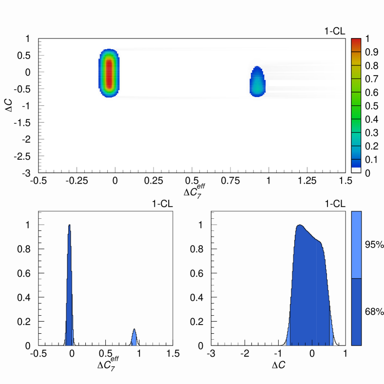
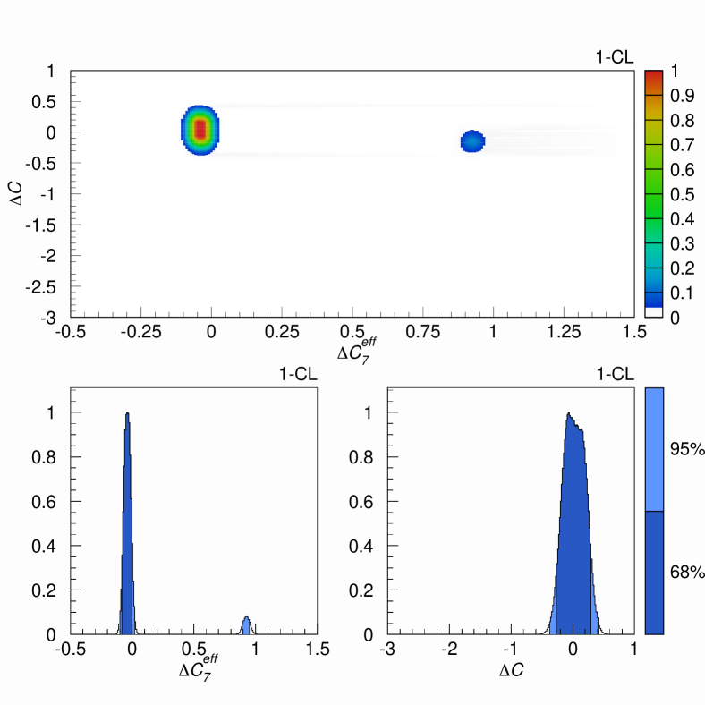
Figure 5: The upper (lower) panel displays future constraints on $\Delta C_{7}^{\rm eff}$ and $\Delta C$ within CMFV scanning $\Delta B^{\nu\bar{\nu}}$ in the range $\pm 0.4$ (set to zero) that are based on flavor observables only. The colors encode the frequentist $1-{\rm CL}$ level and the corresponding $68\%$ and $95\%$ probability regions as indicated by the bars on the right side of the panels. See text for details.

It is easy to verify that the derived $95\%\,{\rm CL}$ bound for $\Delta C$ holds in each CMFV model discussed here. By explicit calculations we find that the allowed range for $\Delta C$ is $[0,0.12]$ and $[0,0.13]$ in the THDM type I and II Bobeth:2001jm , $[-0.05,0.06]$ in the MSSM Buras:2000qz , $[0,0.04]$ in the mUED scenario Buras:2002ej , and $[-0.07,0]$ in the LHT model Blanke:2006eb with degenerate mirror fermions.

Other theoretical clean observables that are sensitive to the magnitude and sign of $\Delta C$ are the forward-backward and energy asymmetries in inclusive and exclusive $b\to sl^{+}l^{-}$ decays wcbsll ; Ali:1991is and the branching ratios of $K_{L}\to\pi^{0}\nu\bar{\nu}$ and $K^{+}\to\pi^{+}\nu\bar{\nu}$ Bobeth:2005ck ; Buras:2004uu .

BaBar and Belle have recently reported measurements of the forward-backward asymmetry $A_{\rm FB}(\bar{B}\to K^{\ast}l^{+}l^{-})$ Aubert:2006vb ; fbabelle . Both collaborations conclude that NP scenarios in which the relative sign of the product of the effective Wilson coefficients $C_{9}^{\rm eff}(m_{b})$ and $C_{10}^{\rm eff}(m_{b})$ is opposite to that of the SM are disfavored at $95\%\ {\rm CL}$. While these results also point towards the exclusion of a large destructive NP contribution to the $Z$-penguin amplitude, it is easy to verify that the present $A_{\rm FB}(\bar{B}\to K^{\ast}l^{+}l^{-})$ constraint is less restrictive than the existing data on $Z\to b\bar{b}$ considered by us. Notice that a combination of the branching ratios and forward-backward asymmetries of inclusive and exclusive $b\to sl^{+}l^{-}$ transitions might in principle also allow one to constrain the size of the NP contributions $\Delta B^{l^{+}l^{-}}$ and $\Delta D$. A detailed study of the impact of all the available $b\to sl^{+}l^{-}$ measurements on the allowed range of $\Delta B^{l^{+}l^{-}}$, $\Delta C$, and $\Delta D$ is however beyond the scope of this article.

The remarkable power of the POs $R_{b}^{0}$, ${\cal A}_{b}$, and $A_{\rm FB}^{0,b}$ in unraveling NP contributions to the universal Inami-Lim function $C$ is probably best illustrated by a comparison to one of the undisputed “heavyweight champions” in this category, the $K^{+}\to\pi^{+}\nu\bar{\nu}$ branching ratio. A careful analysis of this decay shows that even under the hypothesis $\Delta B^{\nu\bar{\nu}}=0$ a future measurement of ${\cal B}(K^{+}\to\pi^{+}\nu\bar{\nu})$ close to its SM prediction with an accuracy of $\pm 10\%$ would only lead to a slightly better $95\%\,{\rm CL}$ bound than the one given in Eq. (16), while already relatively small deviations of $B^{\nu\bar{\nu}}$ from its SM value would give the $Z\to b\bar{b}$ POs the edge. This feature is illustrated in Fig. 5 which shows the constraints on $\Delta C$ and $\Delta C_{7}^{\rm eff}$ following from the simultaneous use of the present ${\cal B}(\bar{B}\to X_{s}\gamma)$ and ${\cal B}(\bar{B}\to X_{s}l^{+}l^{-})$ world averages and a future accurate measurement of $K^{+}\to\pi^{+}\nu\bar{\nu}$ leading to ${\cal B}(K^{+}\to\pi^{+}\nu\bar{\nu})=(7.63\pm 0.76)\times 10^{-11}$. In the upper (lower) panel the contribution $\Delta B^{\nu\bar{\nu}}$ is allowed to float freely in the range $\pm 0.4$ (set to zero). In the former case we find the following $\Delta C$ bounds

$$\Delta C =-0.057\pm 0.588 \!\!(68\%\,{\rm CL})\,,$$ (18)

$$\Delta C =[-0.768,0.668] \!\!(95\%\,{\rm CL})\,,$$

while in the latter one we arrive at

$$\Delta C =0.026\pm 0.282 \!\!(68\%\,{\rm CL})\,,$$ (19)

$$\Delta C =[-0.376,0.420] \!\!(95\%\,{\rm CL})\,.$$

However, this “upset” of the $K^{+}\to\pi^{+}\nu\bar{\nu}$ mode should not be over emphasized. While in MFV models the rates of the rare $K\to\pi\nu\bar{\nu}$ decays can be enhanced only moderately Bobeth:2005ck ; Isidori:2006qy a very different picture can emerge in non-MFV scenarios with new sources of flavor and $CP$ violation. Since now the hard GIM mechanism present in the MFV $s\to d\nu\bar{\nu}$ decay amplitude is in general no longer active, large departures from the SM predictions are still possible without violating any existing experimental constraint Blanke:2006eb ; kpnnnonmfv . Precise measurements of the processes $K^{+}\to\pi^{+}\nu\bar{\nu}$ and $K_{L}\to\pi^{0}\nu\bar{\nu}$ will therefore have a non-trivial impact on our understanding of the flavor structure and $CP$ violation of NP well above the ${\rm TeV}$ scale. This statement remains true even after taking into account possible future constraints on the mass spectrum obtained at the LHC and the refinement of the flavor constraints expected from the $B$-factories Isidori:2006qy ; Blanke:2006eb .

Table 3: Bounds for various rare decays in CMFV models at $95\%$ probability, the corresponding values in the SM at $68\%$ and $95\%\,{\rm CL}$, and the available experimental information. See text for details.

Observable	CMFV ($95\%\,{\rm CL}$)	SM ($68\%\,{\rm CL}$)	SM ($95\%\,{\rm CL}$)	Experiment
${\cal B}(K^{+}\to\pi^{+}\nu\bar{\nu})\times 10^{11}$	$[4.29,10.72]$	$7.15\pm 1.28$	$[5.40,9.11]$	$\left(14.7^{+13.0}_{-8.9}\right)$ kp
${\cal B}(K_{L}\to\pi^{0}\nu\bar{\nu})\times 10^{11}$	$[1.55,4.38]$	$2.79\pm 0.31$	$[2.21,3.45]$	$<2.1\times 10^{4}\;\;(90\%\,\text{CL})$ Ahn:2006uf
${\cal B}(K_{L}\to\mu^{+}\mu^{-})_{\rm SD}\times 10^{9}$	$[0.30,1.22]$	$0.70\pm 0.11$	$[0.54,0.88]$	–
${\cal B}(\bar{B}\to X_{d}\nu\bar{\nu})\times 10^{6}$	$[0.77,2.00]$	$1.34\pm 0.05$	$[1.24,1.45]$	–
${\cal B}(\bar{B}\to X_{s}\nu\bar{\nu})\times 10^{5}$	$[1.88,4.86]$	$3.27\pm 0.11$	$[3.06,3.48]$	$<64\;\;(90\%\,\text{CL})$ Barate:2000rc
${\cal B}(B_{d}\to\mu^{+}\mu^{-})\times 10^{10}$	$[0.36,2.03]$	$1.06\pm 0.16$	$[0.87,1.27]$	$<3.0\times 10^{2}\;\;(95\%\,\text{CL})$ Bernhard:2006fa
${\cal B}(B_{s}\to\mu^{+}\mu^{-})\times 10^{9}$	$[1.17,6.67]$	$3.51\pm 0.50$	$[2.92,4.13]$	$<9.3\times 10^{1}\;\;(95\%\,\text{CL})$ Sanchez:2007ew

In order to allow a better comparison with the results presented previously in Bobeth:2005ck , we will set $\Delta B^{\nu\bar{\nu}}=\Delta B^{l^{+}l^{-}}=0$ when determining the allowed ranges for the branching ratios of $K^{+}\to\pi^{+}\nu\bar{\nu}$, $K_{L}\to\pi^{0}\nu\bar{\nu}$, $K_{L}\to\mu^{+}\mu^{-}$, $\bar{B}\to X_{d,s}\nu\bar{\nu}$, and $B_{d,s}\to\mu^{+}\mu^{-}$ within CMFV. The corresponding lower and upper bounds at $95\%$ probability are reported in Tab. 3. For comparison, we also show the $68\%$ and $95\%\ {\rm CL}$ limits in the SM, obtained using the CKM parameters from a standard UT analysis. The calculations of the SM branching ratios all employ the results of XY . In addition we take into account the recent theoretical developments of Isidori:2005xm ; bghn ; Mescia:2007kn in the case of $K^{+}\to\pi^{+}\nu\bar{\nu}$ and $K_{L}\to\pi^{0}\nu\bar{\nu}$, and of Gorbahn:2006bm for what concerns $K_{L}\to\mu^{+}\mu^{-}$. In contrast to the standard approach we normalize the $\bar{B}\to X_{d,s}\nu\bar{\nu}$ decay width to the $\bar{B}\to X_{u}e\bar{\nu}$ rate, while we follow Buras:2003td in the case of $B_{d,s}\to\mu^{+}\mu^{-}$, since both procedures lead to a reduction of theoretical uncertainties. The actual numerical analysis is performed with a modified version of the CKMfitter code. The used input parameters are given in App. B.

It is evident from Tab. 3 that the strong bound on $\Delta C$, coming mainly from the existing precision measurements of the $Z\to b\bar{b}$ POs, does only allow for CMFV departures relative to the SM branching ratios that range from around $\pm 20\%$ to at most $\pm 60\%$ for the given rare $K$- and $B$-decays. While our upper bounds are in good agreement with the results of Bobeth:2005ck , the derived lower bounds are one of the new results of our article. A strong violation of any of the $95\%\ {\rm CL}$ bounds on the considered branching ratios by future measurements will imply a failure of the CMFV assumption, signaling either the presence of new effective operators and/or new flavor and $CP$ violation. A way to evade the given limits is the presence of sizable corrections $\delta C_{\rm NP}$ and/or $\Delta B^{\nu\bar{\nu}}$ and $\Delta B^{l^{+}l^{-}}$. While these possibilities cannot be fully excluded, general arguments and explicit calculations indicate that they are both difficult to realize in the CMFV framework.

V Conclusions

To conclude, we have pointed out that large contributions to the universal Inami-Lim function $C$ in constrained minimal-flavor-violation that would reverse the sign of the standard $Z$-penguin amplitude are highly disfavored by the existing measurements of the pseudo observables $R_{b}^{0}$, ${\cal A}_{b}$, and $A_{\rm FB}^{0,b}$ performed at LEP and SLC. This underscores the outstanding role of electroweak precision tests in guiding us toward the right theory and immediately raises the question: What else can flavor physics learn from the high-energy frontier?

Appendix A Vertex functions

Below we present the analytic expressions for the non-universal contributions to the renormalized LH $Zd_{j}\bar{d_{i}}$ vertex functions in the CMFV models considered in this article. All expressions correspond to the limit of on-shell external quarks with vanishing mass and have been obtained in the ’t Hooft-Feynman gauge.

In the THDM type I, the only additional non-universal contribution to the $Z\to d_{j}\bar{d}_{i}$ transitions stems from diagrams with charged Higgs boson, $H^{\pm}$, and top quark, $t$, exchange. An example of such a graph is shown on the top left-hand side of Fig. 2. The correction depends on the mass of the charged Higgs boson, $M_{H}^{\pm}$, the top quark mass, $m_{t}$, and on the ratio of the vacuum expectation value of the Higgs doublets, $\tan\beta$. Using the decomposition of Eq. (7) we find for the corresponding form factor

$$C_{\rm THDM}(q^{2}) =\frac{\tan^{2}\beta}{96}\frac{m_{t}^{2}}{M_{\scriptscriptstyle W}^{2}}\scalebox{1.0}{\Bigg{[}}\frac{(22s_{\scriptscriptstyle W}^{2}-9)M_{H}^{\pm 2}-3\,(6s_{\scriptscriptstyle W}^{2}-1)m_{t}^{2}}{M_{H}^{\pm 2}-m_{t}^{2}}$$

$$+\frac{2\,(2s_{\scriptscriptstyle W}^{2}-3)\left(2M_{H}^{\pm 4}-(4m_{t}^{2}+q^{2})M_{H}^{\pm 2}+2(m_{t}^{2}+q^{2})m_{t}^{2}\right)}{(M_{H}^{\pm 2}-m_{t}^{2})^{2}q^{2}}A_{0}(M_{H}^{\pm 2})$$

$$-\frac{2\,(2s_{\scriptscriptstyle W}^{2}-3)\left(2M_{H}^{\pm 4}-4M_{H}^{\pm 2}m_{t}^{2}+2m_{t}^{4}+m_{t}^{2}q^{2}\right)}{(M_{H}^{\pm 2}-m_{t}^{2})^{2}q^{2}}A_{0}(m_{t}^{2})$$

$$-\frac{6\,(2s_{\scriptscriptstyle W}^{2}-1)\left(2M_{H}^{\pm 2}-2m_{t}^{2}-q^{2}\right)}{q^{2}}B_{0}(q^{2},M_{H}^{\pm 2},M_{H}^{\pm 2})$$

$$+\frac{8s_{\scriptscriptstyle W}^{2}\left(2M_{H}^{\pm 2}-2m_{t}^{2}-q^{2}\right)}{q^{2}}B_{0}(q^{2},m_{t}^{2},m_{t}^{2})$$

$$+\frac{12\,(2s_{\scriptscriptstyle W}^{2}-1)\left(M_{H}^{\pm 4}-2M_{H}^{\pm 2}m_{t}^{2}+m_{t}^{4}+m_{t}^{2}q^{2}\right)}{q^{2}}\hskip 1.42262ptC_{0}(q^{2},0,0,M_{H}^{\pm 2},M_{H}^{\pm 2},m_{t}^{2})$$

$$+\frac{4\left(4s_{\scriptscriptstyle W}^{2}M_{H}^{\pm 4}+4s_{\scriptscriptstyle W}^{2}m_{t}^{4}-\left(8s_{\scriptscriptstyle W}^{2}M_{H}^{\pm 2}-(4s_{\scriptscriptstyle W}^{2}-3)q^{2}\right)m_{t}^{2}\right)}{q^{2}}\hskip 1.42262ptC_{0}(q^{2},0,0,m_{t}^{2},m_{t}^{2},M_{H}^{\pm 2})\scalebox{1.0}{\Bigg{]}}\,.$$ (20)

Here and in the following the coefficients $A_{0}(m^{2})$, $B_{0}(p^{2},m_{1}^{2},m_{2}^{2})$, and $C_{0}(p_{1}^{2},p_{2}^{2},(p_{1}+p_{2})^{2},m_{1}^{2},m_{2}^{2},m_{3}^{2})$ denote the finite parts of the scalar one-, two-, and three-point functions in the $\overline{\rm MS}$ scheme as implemented in LoopTools Hahn:1998yk and FF vanOldenborgh:1990yc . The above result agrees with the findings of Denner:1991ie . In the case of the THDM type II the overall factor $\tan^{2}\beta$ has to be replaced by $\cot^{2}\beta$.

In the case of the MSSM only SUSY diagrams involving chargino, $\tilde{\chi}^{\pm}_{m}$, and up-squark, $\tilde{u}_{a}$, exchange lead to non-universal correction to the renormalized LH $Zd_{j}\bar{d_{i}}$ vertex of Eq. (7). An example of a possible contribution can be seen on the top right side of Fig. 2. The corresponding form factor can be written as

$$C_{\tilde{\chi}^{\pm}}(q^{2}) =-\frac{\kappa_{ij}e^{2}}{4M_{\scriptscriptstyle W}^{2}}\sum_{m,n=1}^{2}\sum_{a,b=1}^{6}(X^{U_{L}\dagger}_{m})_{jb}(X^{U_{L}}_{n})_{ai}\scalebox{1.185}{\Bigg{\{}}2M_{\tilde{\chi}_{n}}^{\pm}M_{\tilde{\chi}_{m}}^{\pm}C_{0}(q^{2},0,0,M_{\tilde{\chi}_{n}}^{\pm 2},M_{\tilde{\chi}_{m}}^{\pm 2},m_{\tilde{u}_{a}}^{2})\hskip 1.42262ptU_{m1}U_{n1}^{\ast}\delta_{ab}$$

$$+\Bigg{[}-\ln(M_{\tilde{\chi}_{n}}^{\pm 2})+\frac{1}{2q^{2}}\bigg{(}3q^{2}+2A_{0}(M_{\tilde{\chi}_{n}}^{\pm 2})+2A_{0}(M_{\tilde{\chi}_{m}}^{\pm 2})-4A_{0}(m_{\tilde{u}_{a}}^{2})$$

$$\hskip 20.00003pt-2\left(M_{\tilde{\chi}_{n}}^{\pm 2}+M_{\tilde{\chi}_{m}}^{\pm 2}-2m_{\tilde{u}_{a}}^{2}+q^{2}\right)B_{0}(q^{2},M_{\tilde{\chi}_{n}}^{\pm 2},M_{\tilde{\chi}_{m}}^{\pm 2})$$

$$\hskip 20.00003pt+4\hskip 1.42262pt(M_{\tilde{\chi}_{n}}^{\pm 2}-m_{\tilde{u}_{a}}^{2})(M_{\tilde{\chi}_{m}}^{\pm 2}-m_{\tilde{u}_{a}}^{2})\hskip 1.42262ptC_{0}(q^{2},0,0,M_{\tilde{\chi}_{n}}^{\pm 2},M_{\tilde{\chi}_{m}}^{\pm 2},m_{\tilde{u}_{a}}^{2})\bigg{)}\Bigg{]}W_{m1}^{\ast}W_{n1}\delta_{ab}$$

$$-\Bigg{[}-\ln(M_{\tilde{\chi}_{n}}^{\pm 2})+\frac{1}{2q^{2}}\bigg{(}q^{2}+4A_{0}(M_{\tilde{\chi}_{n}}^{\pm 2})-2A_{0}(m_{\tilde{u}_{a}}^{2})-2A_{0}(m_{\tilde{u}_{b}}^{2})$$

$$\hskip 20.00003pt-2\left(2M_{\tilde{\chi}_{n}}^{\pm 2}-m_{\tilde{u}_{a}}^{2}-m_{\tilde{u}_{b}}^{2}+q^{2}\right)B_{0}(q^{2},m_{\tilde{u}_{a}}^{2},m_{\tilde{u}_{b}}^{2})$$

$$\hskip 20.00003pt-4\left(M_{\tilde{\chi}_{n}}^{\pm 4}+m_{\tilde{u}_{a}}^{2}m_{\tilde{u}_{b}}^{2}-\left(m_{\tilde{u}_{a}}^{2}+m_{\tilde{u}_{b}}^{2}-q^{2}\right)M_{\tilde{\chi}_{n}}^{\pm 2}\right)\hskip 1.42262ptC_{0}(q^{2},0,0,m_{\tilde{u}_{a}}^{2},m_{\tilde{u}_{b}}^{2},M_{\tilde{\chi}_{n}}^{\pm 2})\bigg{)}\Bigg{]}(\Gamma^{U_{L}}{\Gamma^{U_{L}\dagger}})_{ba}\delta_{mn}\hskip 21.33955pt$$

$$+\Bigg{[}\frac{-(22s_{\scriptscriptstyle W}^{2}-9)\hskip 1.42262ptM_{\tilde{\chi}_{n}}^{\pm 2}+3\hskip 1.42262pt(6s_{\scriptscriptstyle W}^{2}-1)\hskip 1.42262ptm_{\tilde{u}_{a}}^{2}}{6(M_{\tilde{\chi}_{n}}^{\pm 2}-m_{\tilde{u}_{a}}^{2})}$$

$$\hskip 20.00003pt-\frac{(2s_{\scriptscriptstyle W}^{2}-3)\left(2M_{\tilde{\chi}_{n}}^{\pm 4}+2m_{\tilde{u}_{a}}^{4}-(4m_{\tilde{u}_{a}}^{2}-q^{2})\hskip 1.42262ptM_{\tilde{\chi}_{n}}^{\pm 2}\right)}{3(M_{\tilde{\chi}_{n}}^{\pm 2}-m_{\tilde{u}_{a}}^{2})^{2}q^{2}}A_{0}(M_{\tilde{\chi}_{n}}^{\pm 2})$$

$$\hskip 20.00003pt+\frac{(2s_{\scriptscriptstyle W}^{2}-3)\left(2M_{\tilde{\chi}_{n}}^{\pm 4}+2m_{\tilde{u}_{a}}^{4}-2\,(2m_{\tilde{u}_{a}}^{2}-q^{2})\hskip 1.42262ptM_{\tilde{\chi}_{n}}^{\pm 2}-m_{\tilde{u}_{a}}^{2}q^{2}\right)}{3(M_{\tilde{\chi}_{n}}^{\pm 2}-m_{\tilde{u}_{a}}^{2})^{2}q^{2}}A_{0}(m_{\tilde{u}_{a}}^{2})$$

$$\hskip 20.00003pt+\frac{(2s_{\scriptscriptstyle W}^{2}-1)\left(2M_{\tilde{\chi}_{n}}^{\pm 2}-2m_{\tilde{u}_{a}}^{2}+q^{2}\right)}{q^{2}}B_{0}(q^{2},M_{\tilde{\chi}_{n}}^{\pm 2},M_{\tilde{\chi}_{n}}^{\pm 2})$$

$$\hskip 20.00003pt-\frac{4s_{\scriptscriptstyle W}^{2}\left(2M_{\tilde{\chi}_{n}}^{\pm 2}-2m_{\tilde{u}_{a}}^{2}+q^{2}\right)}{3q^{2}}B_{0}(q^{2},m_{\tilde{u}_{a}}^{2},m_{\tilde{u}_{a}}^{2})$$

$$\hskip 20.00003pt-\frac{2\,(2s_{\scriptscriptstyle W}^{2}-1)\left(M_{\tilde{\chi}_{n}}^{\pm 4}+m_{\tilde{u}_{a}}^{4}-(2m_{\tilde{u}_{a}}^{2}-q^{2})\hskip 1.42262ptM_{\tilde{\chi}_{n}}^{2}\right)}{q^{2}}C_{0}(q^{2},0,0,M_{\tilde{\chi}_{n}}^{\pm 2},M_{\tilde{\chi}_{n}}^{\pm 2},m_{\tilde{u}_{a}}^{2})$$

$$\hskip 20.00003pt-\frac{8s_{\scriptscriptstyle W}^{2}\left(M_{\tilde{\chi}_{n}}^{\pm 4}+m_{\tilde{u}_{a}}^{4}-(2m_{\tilde{u}_{a}}^{2}-q^{2})\hskip 1.42262ptM_{\tilde{\chi}_{n}}^{\pm 2}\right)}{3q^{2}}C_{0}(q^{2},0,0,m_{\tilde{u}_{a}}^{2},m_{\tilde{u}_{a}}^{2},M_{\tilde{\chi}_{n}}^{\pm 2})\Bigg{]}\delta_{ab}\delta_{mn}\scalebox{1.185}{\Bigg{\}}}\,,$$ (21)

where $\kappa_{ij}\equiv(8\sqrt{2}G_{F}e^{2}V^{\ast}_{tj}V_{ti})^{-1}$ with $V$ being the CKM matrix and $i,j=d,s,b$.

The LH chargino-up-squark-down-quark coupling matrix takes the form

$$X_{n}^{U_{L}}=-\frac{e}{s_{\scriptscriptstyle W}}\left(W_{n1}^{\ast}\Gamma^{U_{L}}-W_{n2}^{\ast}\Gamma^{U_{R}}\frac{M_{U}}{\sqrt{2}M_{\scriptscriptstyle W}s_{\beta}}\right)V\,.\hskip 7.11317pt$$ (22)

Here and in the following $s_{\beta}\equiv\sin\beta$, $c_{\beta}\equiv\cos\beta$, $t_{\beta}\equiv\tan\beta$, etc.

The unitary mixing matrices $U$ and $W$ are defined through

$$U^{\ast}M_{\tilde{\chi}^{\pm}}W^{\dagger}={\rm diag}(M_{\tilde{\chi}_{1}}^{\pm},M_{\tilde{\chi}_{2}}^{\pm})\,,$$ (23)

with $M_{\tilde{\chi}_{1,2}}^{\pm}$ being the physical chargino masses that satisfy $M^{\pm}_{\tilde{\chi}_{1}}<M^{\pm}_{\tilde{\chi}_{2}}$. $M_{\tilde{\chi}^{\pm}}$ denotes the chargino mass matrix, which in terms of the wino, $M_{2}$, and higgsino mass parameter, $\mu$, reads

$$M_{\tilde{\chi}^{\pm}}=\begin{pmatrix}M_{2}&\sqrt{2}M_{\scriptscriptstyle W}s_{\beta}\\ \sqrt{2}M_{\scriptscriptstyle W}c_{\beta}&\mu\end{pmatrix}\,.$$ (24)

The $6\times 3$ matrices

$$(\Gamma^{U_{L}})_{ai}=(\Gamma^{U})_{ai}\,,\hskip 14.22636pt(\Gamma^{U_{R}})_{ai}=(\Gamma^{U})_{a,i+3}\,.$$ (25)

are building blocks of the unitary matrix $\Gamma^{U}$ that diagonalizes the $6\times 6$ mass-squared matrix $M^{2}_{\tilde{U}}$ of the up-type squarks:

$$\Gamma^{U}M_{\tilde{U}}^{2}{\Gamma^{U}}^{\dagger}={\rm diag}(m_{\tilde{u}_{1}}^{2},\dots,m_{\tilde{u}_{6}}^{2})\,.$$ (26)

In the super-CKM basis Misiak:1997ei , $M^{2}_{\tilde{U}}$ is given by

$$M^{2}_{\tilde{U}}=\begin{pmatrix}M_{\tilde{U}_{L}}^{2}+M_{U}^{2}+M_{\scriptscriptstyle Z}^{2}\hskip 1.42262ptc_{2\beta}\left(\frac{1}{2}-\frac{2}{3}s^{2}_{\scriptscriptstyle W}\right)\leavevmode\hbox{\small 1\kern-3.6pt\normalsize 1}&M_{U}\left(A_{U}^{\ast}-\mu\hskip 1.42262ptt_{\beta}^{-1}\leavevmode\hbox{\small 1\kern-3.6pt\normalsize 1}\right)\\ \left[M_{U}\left(A_{U}^{\ast}-\mu\hskip 1.42262ptt_{\beta}^{-1}\leavevmode\hbox{\small 1\kern-3.6pt\normalsize 1}\right)\right]^{\dagger}&M_{\tilde{U}_{R}}^{2}+M_{U}^{2}+\frac{2}{3}M_{\scriptscriptstyle Z}^{2}\hskip 1.42262ptc_{2\beta}s^{2}_{\scriptscriptstyle W}\leavevmode\hbox{\small 1\kern-3.6pt\normalsize 1}\end{pmatrix}\,,$$ (27)

where $M_{\tilde{U}_{L}}=m_{\tilde{Q}_{L}}\leavevmode\hbox{\small 1\kern-3.6pt\normalsize 1}$ and $M_{\tilde{U}_{R}}=m_{\tilde{u}_{R}}\leavevmode\hbox{\small 1\kern-3.6pt\normalsize 1}$ are the left and right soft SUSY breaking up-type squark mass matrices, $M_{U}={\rm diag}(m_{u},m_{c},m_{t})$, $A_{U}=A_{u}\leavevmode\hbox{\small 1\kern-3.6pt\normalsize 1}$ contains the trilinear parameters and 11 represents the $3\times 3$ unit matrix. We assume $CP$ conservation, so all soft SUSY breaking terms are real.

The result given in Eq. (A) agrees with the one of Boulware:1991vp . To verify the consistency of the results one has to take into account that in the last equation of Boulware:1991vp the coefficient $C_{11}$ should read $C_{12}$, and that arbitrary constant terms can be added to the second and third coefficient of the four different coupling structures in Eq. (A), since their contribution disappears after the summations over $m,n,a$, and $b$ have been performed. In addition, the explicit $\ln(M_{\tilde{\chi}_{n}}^{\pm 2})$ terms are absent in Boulware:1991vp . They have been chosen such that $C_{\tilde{\chi}^{\pm}}(q^{2})$ coincides for $q^{2}=0$ with the expression for the one-loop $Z$-penguin function given in Bobeth:2001jm .

In the mUED model diagrams containing infinite towers of the KK modes corresponding to the $W$-boson, $W^{\pm}_{(k)}$, the pseudo Goldstone boson, $G^{\pm}_{(k)}$, the $SU(2)$ quark doublets, ${\cal Q}_{q(k)}$, and the $SU(2)$ quark singlets, ${\cal U}_{q(k)}$, as well as the charged scalar, $a^{\pm}_{(k)}$, contribute to the non-universal correction to the $Zd_{j}\bar{d_{i}}$ vertex. A possible diagram can be seen on the lower left side in Fig. 2. The only additional parameter entering the form factor in Eq. (7) relative to the SM is the inverse of the compactification radius $1/R$. We obtain

$$C_{\rm mUED}(q^{2}) =\frac{1}{96}\sum^{\infty}_{k=1}\scalebox{1.185}{\Bigg{[}}\frac{\left(-8\,(2s_{\scriptscriptstyle W}^{2}-3)m_{(k)}^{2}-(34s_{\scriptscriptstyle W}^{2}-27)M_{\scriptscriptstyle W}^{2}+3\,(6s_{\scriptscriptstyle W}^{2}-1)m_{t}^{2}\right)m_{t}^{2}}{(m_{t}^{2}-M_{\scriptscriptstyle W}^{2})M_{\scriptscriptstyle W}^{2}}$$

$$-\frac{2\,(2s_{\scriptscriptstyle W}^{2}-3)}{(m_{t}^{2}-M_{\scriptscriptstyle W}^{2})^{2}M_{\scriptscriptstyle W}^{2}q^{2}}\Big{(}2m_{t}^{6}+(2M_{\scriptscriptstyle W}^{2}+q^{2})m_{t}^{4}-5\,(2M_{\scriptscriptstyle W}^{2}+q^{2})\hskip 1.42262ptm_{t}^{2}M_{\scriptscriptstyle W}^{2}$$

$$\hskip 50.00008pt+6M_{\scriptscriptstyle W}^{6}+(m_{t}^{2}+3M_{\scriptscriptstyle W}^{2})\hskip 1.42262ptm_{(k)}^{2}q^{2}+8M_{\scriptscriptstyle W}^{4}q^{2}\Big{)}A_{0}(m_{t(k)}^{2})$$

$$+\frac{2\,(2s_{\scriptscriptstyle W}^{2}-3)\left(\left(2m_{t}^{4}-(4M_{\scriptscriptstyle W}^{2}+3q^{2})m_{t}^{2}+2M_{\scriptscriptstyle W}^{4}+7M_{\scriptscriptstyle W}^{2}q^{2}\right)M_{\scriptscriptstyle W}^{2}+(7M_{\scriptscriptstyle W}^{2}-3m_{t}^{2})\hskip 1.42262ptm_{(k)}^{2}q^{2}\right)m_{t}^{2}}{(m_{t}^{2}-M_{\scriptscriptstyle W}^{2})^{2}M_{\scriptscriptstyle W}^{4}q^{2}}A_{0}(M_{{\scriptscriptstyle W}(k)}^{2})$$

$$+\frac{2\,(2s_{\scriptscriptstyle W}^{2}-3)\left(6M_{\scriptscriptstyle W}^{4}+3m_{(k)}^{2}q^{2}+8M_{\scriptscriptstyle W}^{2}q^{2}\right)}{M_{\scriptscriptstyle W}^{4}q^{2}}A_{0}(m_{(k)}^{2})$$

$$-\frac{2\left(8s_{\scriptscriptstyle W}^{2}m_{t}^{4}+2\left((8s_{\scriptscriptstyle W}^{2}-9)M_{\scriptscriptstyle W}^{2}+2s_{\scriptscriptstyle W}^{2}q^{2}\right)m_{t}^{2}-(4s_{\scriptscriptstyle W}^{2}-3)(6M_{\scriptscriptstyle W}^{2}+5q^{2})M_{\scriptscriptstyle W}^{2}\right)}{M_{\scriptscriptstyle W}^{2}q^{2}}B_{0}(q^{2},m_{t(k)}^{2},m_{t(k)}^{2})$$

$$+\frac{6\left((4s_{\scriptscriptstyle W}^{2}-2)\hskip 1.42262ptm_{t}^{2}+2(4s_{\scriptscriptstyle W}^{2}-5)M_{\scriptscriptstyle W}^{2}+(2s_{\scriptscriptstyle W}^{2}-1)\hskip 1.42262ptq^{2}\right)m_{t}^{2}}{M_{\scriptscriptstyle W}^{2}q^{2}}B_{0}(q^{2},M_{{\scriptscriptstyle W}(k)}^{2},M_{{\scriptscriptstyle W}(k)}^{2})$$

$$-\frac{2\,(4s_{\scriptscriptstyle W}^{2}-3)(6M_{\scriptscriptstyle W}^{2}+5q^{2})}{q^{2}}B_{0}(q^{2},m_{(k)}^{2},m_{(k)}^{2})$$ (28)

$$+\frac{4}{M_{\scriptscriptstyle W}^{2}q^{2}}\Big{(}4s_{\scriptscriptstyle W}^{2}m_{t}^{6}+\left((4s_{\scriptscriptstyle W}^{2}-9)M_{\scriptscriptstyle W}^{2}+(4s_{\scriptscriptstyle W}^{2}-3)\hskip 1.42262ptq^{2}\right)m_{t}^{4}$$

$$\hskip 50.00008pt-2\left((10s_{\scriptscriptstyle W}^{2}-9)M_{\scriptscriptstyle W}^{4}-2s_{\scriptscriptstyle W}^{2}m_{(k)}^{2}q^{2}+2\,(s_{\scriptscriptstyle W}^{2}-3)M_{\scriptscriptstyle W}^{2}q^{2}\right)m_{t}^{2}$$

$$\hskip 50.00008pt+(4s_{\scriptscriptstyle W}^{2}-3)\left(3M_{\scriptscriptstyle W}^{4}+3m_{(k)}^{2}q^{2}+4M_{\scriptscriptstyle W}^{2}q^{2}+2q^{4}\right)M_{\scriptscriptstyle W}^{2}\Big{)}C_{0}(q^{2},0,0,m_{t(k)}^{2},m_{t(k)}^{2},M_{{\scriptscriptstyle W}(k)}^{2})$$

$$+\frac{12}{M_{\scriptscriptstyle W}^{2}q^{2}}\Big{(}(2s_{\scriptscriptstyle W}^{2}-1)m_{t}^{6}+\left(2\,(s_{\scriptscriptstyle W}^{2}-2)M_{\scriptscriptstyle W}^{2}+(2s_{\scriptscriptstyle W}^{2}-1)\hskip 1.42262ptq^{2}\right)m_{t}^{4}$$

$$\hskip 50.00008pt-\left((10s_{\scriptscriptstyle W}^{2}-11)M_{\scriptscriptstyle W}^{4}-(2s_{\scriptscriptstyle W}^{2}-1)m_{(k)}^{2}q^{2}+2\,(s_{\scriptscriptstyle W}^{2}+1)M_{\scriptscriptstyle W}^{2}q^{2}\right)m_{t}^{2}$$

$$\hskip 50.00008pt-2c_{\scriptscriptstyle W}^{2}\left(3M_{\scriptscriptstyle W}^{4}+3m_{(k)}^{2}q^{2}+4M_{\scriptscriptstyle W}^{2}q^{2}\right)M_{\scriptscriptstyle W}^{2}\Big{)}\hskip 1.42262ptC_{0}(q^{2},0,0,M_{{\scriptscriptstyle W}(k)}^{2},M_{{\scriptscriptstyle W}(k)}^{2},m_{t(k)}^{2})$$

$$+\frac{24\,c_{\scriptscriptstyle W}^{2}\left(3M_{\scriptscriptstyle W}^{4}+3m_{(k)}^{2}q^{2}+4M_{\scriptscriptstyle W}^{2}q^{2}\right)}{q^{2}}\hskip 1.42262ptC_{0}(q^{2},0,0,M_{{\scriptscriptstyle W}(k)}^{2},M_{{\scriptscriptstyle W}(k)}^{2},m_{(k)}^{2})$$

$$-\frac{4\,(4s_{\scriptscriptstyle W}^{2}-3)\left(3M_{\scriptscriptstyle W}^{4}+3m_{(k)}^{2}q^{2}+4M_{\scriptscriptstyle W}^{2}q^{2}+2q^{4}\right)}{q^{2}}\hskip 1.42262ptC_{0}(q^{2},0,0,m_{(k)}^{2},m_{(k)}^{2},M_{{\scriptscriptstyle W}(k)}^{2})\scalebox{1.185}{\Bigg{]}}\,,$$

where $m_{t(k)}=\sqrt{m_{t}^{2}+m_{(k)}^{2}}$, $M_{{\scriptscriptstyle W}(k)}=\sqrt{M_{\scriptscriptstyle W}^{2}+m_{(k)}^{2}}$, and $m_{(k)}=k/R$. We note that our new result for $C_{\rm mUED}(q^{2})$ coincides for $q^{2}=0$ with the one-loop KK contribution to the $Z$-penguin function found in Buras:2002ej .

In the case of the LHT with degenerate mirror fermions the only new particle that effects the $Z\to d_{j}\bar{d}_{i}$ transition in a non-universal way is a $T$-even heavy top, $T_{+}$. A sample diagram involving such a fermion is given on the lower right-hand side of Fig. 2. The form factor depends on the mass of the heavy top, which is controlled by the size of the top Yukawa coupling, the symmetry breaking scale $f$, and the parameter $x_{L}\equiv\lambda_{1}^{2}/(\lambda_{1}^{2}+\lambda_{2}^{2})$. Here $\lambda_{1}$ is the Yukawa coupling between $t$ and $T_{+}$ and $\lambda_{2}$ parametrizes the mass term of $T_{+}$. Our result for the form factor entering Eq. (7) is given by

$$C_{\rm LHT}(q^{2}) =\frac{x^{2}_{L}}{96}\frac{v^{2}}{f^{2}}\scalebox{1.185}{\Bigg{[}}\frac{3(M^{2}_{T_{+}}-m_{t}^{2})\left(\left((6s_{\scriptscriptstyle W}^{2}-1)M^{2}_{T_{+}}-(10s_{\scriptscriptstyle W}^{2}-7)M_{\scriptscriptstyle W}^{2}\right)M_{\scriptscriptstyle W}^{2}-(6s_{\scriptscriptstyle W}^{2}-1)(M^{2}_{T_{+}}-M_{\scriptscriptstyle W}^{2})\hskip 1.42262ptm_{t}^{2}\right)}{(M^{2}_{T_{+}}-M_{\scriptscriptstyle W}^{2})(m_{t}^{2}-M_{\scriptscriptstyle W}^{2})M_{\scriptscriptstyle W}^{2}}$$

$$+\frac{2\,(2s_{\scriptscriptstyle W}^{2}-3)\left(2M^{6}_{T_{+}}+M^{4}_{T_{+}}q^{2}-6(M_{\scriptscriptstyle W}^{2}+q^{2})M^{2}_{T_{+}}M_{\scriptscriptstyle W}^{2}+4(M_{\scriptscriptstyle W}^{2}+2q^{2})M_{\scriptscriptstyle W}^{4}\right)}{(M^{2}_{T_{+}}-M_{\scriptscriptstyle W}^{2})^{2}M_{\scriptscriptstyle W}^{2}q^{2}}A_{0}(M^{2}_{T_{+}})$$

$$-\frac{2\,(2s_{\scriptscriptstyle W}^{2}-3)\left(2m_{t}^{6}+m_{t}^{4}q^{2}-6(M_{\scriptscriptstyle W}^{2}+q^{2})\hskip 1.42262ptm_{t}^{2}M_{\scriptscriptstyle W}^{2}+4(M_{\scriptscriptstyle W}^{2}+2q^{2})M_{\scriptscriptstyle W}^{4}\right)}{(m_{t}^{2}-M_{\scriptscriptstyle W}^{2})^{2}M_{\scriptscriptstyle W}^{2}q^{2}}A_{0}(m_{t}^{2})$$

$$+\frac{2\,(2s_{\scriptscriptstyle W}^{2}-3)(m_{t}^{2}-M^{2}_{T_{+}})}{(M^{2}_{T_{+}}-M_{\scriptscriptstyle W}^{2})^{2}(m_{t}^{2}-M_{\scriptscriptstyle W}^{2})^{2}M_{\scriptscriptstyle W}^{2}q^{2}}\Big{(}2(M^{2}_{T_{+}}-M_{\scriptscriptstyle W}^{2})^{2}m_{t}^{4}$$

$$\hskip 50.00008pt-\left(4M^{4}_{T_{+}}-(8M_{\scriptscriptstyle W}^{2}+q^{2})M^{2}_{T_{+}}+4(M_{\scriptscriptstyle W}^{2}+q^{2})M_{\scriptscriptstyle W}^{2}\right)m_{t}^{2}M_{\scriptscriptstyle W}^{2}$$

$$\hskip 50.00008pt+\left(2M^{4}_{T_{+}}-4(M_{\scriptscriptstyle W}^{2}+q^{2})M^{2}_{T_{+}}+2M_{\scriptscriptstyle W}^{4}+7M_{\scriptscriptstyle W}^{2}q^{2}\right)M_{\scriptscriptstyle W}^{4}\Big{)}A_{0}(M_{\scriptscriptstyle W}^{2})$$

$$+\frac{8s_{\scriptscriptstyle W}^{2}\left(2M^{4}_{T_{+}}+(2M_{\scriptscriptstyle W}^{2}+q^{2})M^{2}_{T_{+}}-4M_{\scriptscriptstyle W}^{4}-6M_{\scriptscriptstyle W}^{2}q^{2}\right)}{M_{\scriptscriptstyle W}^{2}q^{2}}B_{0}(q^{2},M^{2}_{T_{+}},M^{2}_{T_{+}})$$

$$-\frac{8\left(2s_{\scriptscriptstyle W}^{2}m_{t}^{4}+(2(s_{\scriptscriptstyle W}^{2}-3)M_{\scriptscriptstyle W}^{2}+s_{\scriptscriptstyle W}^{2}q^{2})\hskip 1.42262ptm_{t}^{2}-(2s_{\scriptscriptstyle W}^{2}-3)(2M_{\scriptscriptstyle W}^{2}+3q^{2})M_{\scriptscriptstyle W}^{2}\right)}{M_{\scriptscriptstyle W}^{2}q^{2}}B_{0}(q^{2},m_{t}^{2},m_{t}^{2})$$

$$-\frac{24\left(M^{2}_{T_{+}}+m_{t}^{2}-2M_{\scriptscriptstyle W}^{2}-3q^{2}\right)}{q^{2}}B_{0}(q^{2},m_{t}^{2},M^{2}_{T_{+}})$$

$$-\frac{6(M^{2}_{T_{+}}-m_{t}^{2})\left((4s_{\scriptscriptstyle W}^{2}-2)(M^{2}_{T_{+}}+m_{t}^{2})+(4s_{\scriptscriptstyle W}^{2}-6)M_{\scriptscriptstyle W}^{2}+(2s_{\scriptscriptstyle W}^{2}-1)q^{2}\right)}{M_{\scriptscriptstyle W}^{2}q^{2}}B_{0}(q^{2},M_{\scriptscriptstyle W}^{2},M_{\scriptscriptstyle W}^{2})$$ (29)

$$-\frac{16s_{\scriptscriptstyle W}^{2}\left(M^{6}_{T_{+}}+M^{4}_{T_{+}}q^{2}-(3M_{\scriptscriptstyle W}^{2}+2q^{2})M^{2}_{T_{+}}M_{\scriptscriptstyle W}^{2}+2(M_{\scriptscriptstyle W}^{2}+q^{2})^{2}M_{\scriptscriptstyle W}^{2}\right)}{M_{\scriptscriptstyle W}^{2}q^{2}}C_{0}(q^{2},0,0,M^{2}_{T_{+}},M^{2}_{T_{+}},M_{\scriptscriptstyle W}^{2})$$

$$+\frac{8}{M_{\scriptscriptstyle W}^{2}q^{2}}\Big{(}2s_{\scriptscriptstyle W}^{2}m_{t}^{6}-(6M_{\scriptscriptstyle W}^{2}-(2s_{\scriptscriptstyle W}^{2}-3)q^{2})\hskip 1.42262ptm_{t}^{4}-2(3(s_{\scriptscriptstyle W}^{2}-2)M_{\scriptscriptstyle W}^{2}+2(s_{\scriptscriptstyle W}^{2}-3)q^{2})\hskip 1.42262ptm_{t}^{2}M_{\scriptscriptstyle W}^{2}$$

$$\hskip 50.00008pt+2(2s_{\scriptscriptstyle W}^{2}-3)(M_{\scriptscriptstyle W}^{2}+q^{2})^{2}M_{\scriptscriptstyle W}^{2}\Big{)}C_{0}(q^{2},0,0,m_{t}^{2},m_{t}^{2},M_{\scriptscriptstyle W}^{2})$$

$$+\frac{24}{M_{\scriptscriptstyle W}^{2}q^{2}}\Big{(}\left((2M_{\scriptscriptstyle W}^{2}+q^{2})M^{2}_{T_{+}}-2(M_{\scriptscriptstyle W}^{2}+q^{2})M_{\scriptscriptstyle W}^{2}\right)\hskip 1.42262ptm_{t}^{2}$$

$$\hskip 50.00008pt-2(M_{\scriptscriptstyle W}^{2}+q^{2})\left(M^{2}_{T_{+}}-M_{\scriptscriptstyle W}^{2}-q^{2}\right)M_{\scriptscriptstyle W}^{2}\Big{)}C_{0}(q^{2},0,0,m_{t}^{2},M^{2}_{T_{+}},M_{\scriptscriptstyle W}^{2})$$

$$-\frac{12}{M_{\scriptscriptstyle W}^{2}q^{2}}\Big{(}(2s_{\scriptscriptstyle W}^{2}-1)M^{6}_{T_{+}}-\left(2M_{\scriptscriptstyle W}^{2}-(2s_{\scriptscriptstyle W}^{2}-1)q^{2}\right)M^{4}_{T_{+}}-\left((6s_{\scriptscriptstyle W}^{2}-7)M_{\scriptscriptstyle W}^{4}+4s_{\scriptscriptstyle W}^{2}M_{\scriptscriptstyle W}^{2}q^{2}\right)M^{2}_{T_{+}}$$

$$\hskip 50.00008pt-4\,c_{\scriptscriptstyle W}^{2}(M_{\scriptscriptstyle W}^{2}+2q^{2})M_{\scriptscriptstyle W}^{4}\Big{)}C_{0}(q^{2},0,0,M_{\scriptscriptstyle W}^{2},M_{\scriptscriptstyle W}^{2},M^{2}_{T_{+}})$$

$$+\frac{12}{M_{\scriptscriptstyle W}^{2}q^{2}}\Big{(}(2s_{\scriptscriptstyle W}^{2}-1)\hskip 1.42262ptm_{t}^{6}-\left(2M_{\scriptscriptstyle W}^{2}-(2s_{\scriptscriptstyle W}^{2}-1)q^{2}\right)m_{t}^{4}-\left((6s_{\scriptscriptstyle W}^{2}-7)M_{\scriptscriptstyle W}^{4}+4s_{\scriptscriptstyle W}^{2}M_{\scriptscriptstyle W}^{2}q^{2}\right)m_{t}^{2}$$

$$\hskip 50.00008pt-4c_{\scriptscriptstyle W}^{2}(M_{\scriptscriptstyle W}^{2}+2q^{2})M_{\scriptscriptstyle W}^{4}\Big{)}C_{0}(q^{2},0,0,M_{\scriptscriptstyle W}^{2},M_{\scriptscriptstyle W}^{2},m_{t}^{2})\scalebox{1.185}{\Bigg{]}}\,,$$

where $M_{T_{+}}=f/v\,m_{t}/\sqrt{x_{L}(1-x_{L})}$ and $v\simeq 246\,{\rm GeV}$. Our new result for $C_{\rm LHT}(q^{2})$ resembles for $q^{2}=0$ the analytic expression of the one-loop correction to the low-energy $Z$-penguin function Blanke:2006eb . Taking into account that the latter result corresponds to unitary gauge while we work in ’t Hooft-Feynman gauge is crucial for this comparison.

Appendix B Numerical inputs

In this appendix we collect the values of the experimental and theoretical parameters used in our numerical analysis. The Higgs mass and the various renormalization scales are scanned independently in the ranges $100\,{\rm GeV}<M_{h}^{0}<600\,{\rm GeV}$, $100\,{\rm GeV}<\mu_{t}<300\,{\rm GeV}$, $40\,{\rm GeV}<\mu_{\scriptscriptstyle W}<160\,{\rm GeV}$, $2.5\,{\rm GeV}<\mu_{b}<10\,{\rm GeV}$, and $1\,{\rm GeV}<\mu_{c}<3\,{\rm GeV}$, respectively.

The other parameters are displayed in Tabs. 4 and 5. Errors are indicated only if varying a given parameter within its $1\hskip 1.13809pt\sigma$ range causes an effect larger than $\pm 0.1\%$ on the corresponding result. When two errors are given, the first is treated as a Gaussian $1\hskip 1.13809pt\sigma$ error and the second as a theoretical uncertainty that is scanned in its range.

Table 4: Parameters that enter the standard and universal UT analysis.

Parameter	Value $\pm$ Error(s)	Reference
$|V_{ud}|$	$0.97377\pm 0.00027$	Yao:2006px
$|V_{us}|$	$0.2257\pm 0.0021$	Yao:2006px
$|V_{cb}|$	$(41.7\pm 0.7)\times 10^{-3}$	Yao:2006px
$|V_{ub}|$	$(4.31\pm 0.30)\times 10^{-3}$	Yao:2006px
$|\epsilon_{K}|$	$(2.232\pm 0.007)\times 10^{-3}$	Yao:2006px
$\Delta m_{K}$	$(3.4833\pm 0.0059)\times 10^{-12}\,{\rm MeV}$	Yao:2006px
$\Delta m_{B_{d}}$	$(0.507\pm 0.004)\,{\rm ps}^{-1}$	Barbiero:2007cr
$\Delta m_{B_{s}}$	$(17.77\pm 0.10\pm 0.07)\,{\rm ps}^{-1}$	unknown:2006ze
$\sin(2\beta)_{b\to c\bar{c}s}$	$0.675\pm 0.026$	Barbiero:2007cr
$m_{K^{0}}$	$(497.648\pm 0.022)\,{\rm MeV}$	Yao:2006px
$m_{B_{d}}$	$(5.2793\pm 0.0007)\,{\rm GeV}$	Yao:2006px
$m_{B_{s}}$	$(5.3696\pm 0.0024)\,{\rm GeV}$	Yao:2006px
$f_{K}$	$(159.8\pm 1.5)\,{\rm MeV}$	Yao:2006px
$f_{B_{d}}\hat{B}_{B_{d}}^{1/2}$	$(244\pm 26)\,{\rm MeV}$	Okamoto:2005zg
$f_{B_{s}}\hat{B}_{B_{s}}^{1/2}$	$(281\pm 21)\,{\rm MeV}$	Dalgic:2006gp
$B_{K}$	$0.79\pm 0.04\pm 0.09$	Dawson:2005za
$\hat{B}_{B_{d}}$	$1.28\pm 0.04\pm 0.09$	Aoki:2003xb
$\hat{B}_{B_{s}}$	$1.30\pm 0.03\pm 0.09$	Aoki:2003xb
$\xi$	$1.210^{+0.047}_{-0.035}$	Okamoto:2005zg
$\eta_{tt}$	$0.5765\pm 0.0065$	Buras:1990fn ; Herrlich
$\eta_{ct}$	$0.47\pm 0.04$	Herrlich
$\eta_{cc}$	$1.56\pm 0.37$	Herrlich
$\eta_{B}$	$0.551\pm 0.007$	Buras:1990fn

Tab. 4 contains the quantities that are relevant for the standard and universal UT analysis. We recall that there is a discrepancy of around $1\hskip 1.13809pt\sigma$ between the value of $|V_{ub}|$ obtained from inclusive and exclusive $b\to ue\bar{\nu}$ transitions. Since $|V_{ub}|$ only enters the standard UT analysis its actual value has no impact on our main results. We therefore use the weighted average of $|V_{ub}|$ given in Yao:2006px . In the case of $f_{B_{d}}\hat{B}_{B_{d}}^{1/2}$ and $\xi$ we take the values quoted in Okamoto:2005zg , which combines the values of the bag parameters $\hat{B}_{B_{d}}$ determined by the JLQCD Collaboration using two light flavors of improved Wilson quarks Aoki:2003xb with the staggered three flavor results for the $B$-meson decay constants $f_{B_{d}}$ obtained by the HPQCD Collaboration Gray:2005ad . The central value and error of $f_{B_{s}}\hat{B}_{B_{s}}^{1/2}$ are taken from the recent publication Dalgic:2006gp of the HPQCD Collaboration. For a critical discussion of hadronic uncertainties in the standard CKM fit we refer to Ball:2006xx .

Table 5: Quantities that are necessary for the calculation of the $Z\to b\bar{b}$ POs and the rare and radiative $K$- and $B$-decays.

Parameter	Value $\pm$ Error(s)	Reference
$G_{F}$	$1.16637\times 10^{-5}\,{\rm GeV}^{-2}$	Yao:2006px
$s^{2}_{\scriptscriptstyle W}$	$0.2324\pm 0.0012$	ewpm
$\alpha_{\rm em}(0)$	$1/137.036$	Yao:2006px
$\Delta\alpha_{\rm had}^{(5)}(M_{\scriptscriptstyle Z})$	$0.02768\pm 0.00022$	Hagiwara:2006jt
$\alpha_{s}(M_{\scriptscriptstyle Z})$	$0.1189\pm 0.0020$	Yao:2006px ; Bethke:2006ac
$M_{\scriptscriptstyle Z}$	$(91.1875\pm 0.0021)\,{\rm GeV}$	ewpm
$M_{\scriptscriptstyle W}$	$(80.405\pm 0.030)\,{\rm GeV}$	Yao:2006px
$m_{t,{\rm pole}}$	$(170.9\pm 1.8)\,{\rm GeV}$	Group:2007bx
$m_{b}^{1S}$	$(4.68\pm 0.03)\,{\rm GeV}$	Bauer:2004ve
$m_{c}(m_{c})$	$(1.224\pm 0.017\pm 0.054)\,{\rm GeV}$	Hoang:2005zw
$m_{\mu}$	$105.66\,{\rm MeV}$	Yao:2006px
${\cal B}(\bar{B}\to X_{c}e\bar{\nu})$	$0.1061\pm 0.0017$	Aubert:2004aw
$C$	$0.58\pm 0.01$	Bauer:2004ve
$\lambda_{1}$	$(-0.27\pm 0.04)\,{\rm GeV}^{2}$	Bauer:2004ve
$\lambda_{2}$	$0.12\,{\rm GeV}^{2}$	Yao:2006px
$\kappa_{L}$	$(2.229\pm 0.017)\times 10^{-10}$	Mescia:2007kn
$\kappa_{+}$	$(5.168\pm 0.025)\times 10^{-11}$	Mescia:2007kn
$\kappa_{\mu}$	$(2.009\pm 0.017)\times 10^{-9}$	Gorbahn:2006bm
$\Delta_{\rm EM}$	$-0.003$	Mescia:2007kn
$\tau(B_{d})$	$(1.527\pm 0.008)\,{\rm ps}$	Barbiero:2007cr
$\tau(B_{s})$	$(1.461\pm 0.040)\,{\rm ps}$	Barbiero:2007cr

Tab. 5 summarizes the remaining parameters that enter the determinations of the $Z\to b\bar{b}$ POs and the rare and radiative $K$- and $B$-decays. In the case of $\alpha_{s}(M_{\scriptscriptstyle Z})$, we adopt the central value from Bethke:2006ac , but rescale the corresponding error by a factor of two to be consistent with Yao:2006px . We recall that the parameters $\kappa_{L}$, $\kappa_{+}$, and $\kappa_{\mu}$ scale like $(\lambda/0.225)^{8}$ and that the values given in Tab. 5 correspond to $\lambda\equiv|V_{us}|=0.225$. This scaling has to be taken into account in order to find consistent results in the case of the rare $K$-decays. The IR finite long-distance QED correction factor $\Delta_{\rm EM}$ entering the prediction of $K^{+}\to\pi^{+}\nu\bar{\nu}$ accounts for photon emission with energies of up to $20\,{\rm MeV}$ Mescia:2007kn . Since $m_{c}(m_{c})$ and the phase-space factor $C\equiv|V_{ub}/V_{cb}|^{2}\,\Gamma(\bar{B}\to X_{u}e\bar{\nu})/\Gamma(\bar{B}\to X_{c}e\bar{\nu})$ are strongly correlated we take both of their values from global analyses of semileptonic $B$-decay spectra Bauer:2004ve ; Hoang:2005zw . However, to be conservative, we treat the errors of $m_{c}(m_{c})$ and $C$ as independent in our fit. If the anti-correlation would be included, the individual uncertainties from $m_{c}(m_{c})$ and $C$ in the branching ratios of $\bar{B}\to X_{s}\gamma$, $\bar{B}\to X_{s}l^{+}l^{-}$, and $\bar{B}\to X_{d,s}\nu\bar{\nu}$ would cancel to a large extent against each other bsg .

References

- (1) M. Golden and L. Randall, Nucl. Phys. B 361, 3 (1991); B. Holdom and J. Terning, Phys. Lett. B 247, 88 (1990); M. E. Peskin and T. Takeuchi, Phys. Rev. Lett. 65, 964 (1990) and Phys. Rev. D 46, 381 (1992); G. Altarelli and R. Barbieri, Phys. Lett. B 253, 161 (1991).
- (2) G. Altarelli, R. Barbieri and F. Caravaglios, Nucl. Phys. B 405, 3 (1993) and Phys. Lett. B 314, 357 (1993).
- (3) S. Schael et al. [ALEPH Collaboration], Phys. Rept. 427, 257 (2006).
- (4) N. Cabibbo, Phys. Rev. Lett. 10, 531 (1963); M. Kobayashi and T. Maskawa, Prog. Theor. Phys. 49, 652 (1973).
- (5) J. Charles et al. [CKMfitter Group], Eur. Phys. J. C 41, 1 (2005) and online update available at http://ckmfitter.in2p3.fr/.
- (6) M. Ciuchini et al. [UTFit Collaboration], JHEP 0107, 013 (2001) and online update available at http://www.utfit.org/.
- (7) R. S. Chivukula and H. Georgi, Phys. Lett. B 188, 99 (1987).
- (8) E. Gabrielli and G. F. Giudice, Nucl. Phys. B 433, 3 (1995) [Erratum-ibid. B 507, 549 (1997)]; A. Ali and D. London, Eur. Phys. J. C 9, 687 (1999).
- (9) A. J. Buras et al., Phys. Lett. B 500, 161 (2001).
- (10) G. D’Ambrosio et al., Nucl. Phys. B 645, 155 (2002).
- (11) A. J. Buras, Acta Phys. Polon. B 34, 5615 (2003) and references therein.
- (12) C. Bobeth et al., Nucl. Phys. B 726, 252 (2005).
- (13) V. Cirigliano et al., Nucl. Phys. B 728, 121 (2005).
- (14) V. Cirigliano, G. Isidori and V. Porretti, Nucl. Phys. B 763, 228 (2007); G. C. Branco et al., JHEP 0709, 004 (2007).
- (15) T. Appelquist, H. C. Cheng and B. A. Dobrescu, Phys. Rev. D 64, 035002 (2001).
- (16) N. Arkani-Hamed et al., JHEP 0207, 034 (2002).
- (17) H. C. Cheng and I. Low, JHEP 0309, 051 (2003) and 0408, 061 (2004).
- (18) I. Low, JHEP 0410, 067 (2004).
- (19) M. Blanke et al., JHEP 0610, 003 (2006).
- (20) M. S. Chanowitz, hep-ph/9905478.
- (21) G. Mann and T. Riemann, Annalen Phys. 40, 334 (1984); J. Bernabeu, A. Pich and A. Santamaria, Phys. Lett. B 200, 569 (1988).
- (22) J. Fleischer and O. V. Tarasov, Z. Phys. C 64, 413 (1994).
- (23) K. Agashe, G. Perez and A. Soni, Phys. Rev. Lett. 93, 201804 (2004) and Phys. Rev. D 71, 016002 (2005); K. Agashe et al., hep-ph/0509117; K. Agashe et al., Phys. Lett. B 641, 62 (2006); M. Carena et al., Nucl. Phys. B 759, 202 (2006); G. Cacciapaglia et al., Phys. Rev. D 75, 015003 (2007); R. Contino, L. Da Rold and A. Pomarol, Phys. Rev. D 75, 055014 (2007).
- (24) T. Hahn, Comput. Phys. Commun. 140, 418 (2001) and http://www.feynarts.de/.
- (25) R. Mertig, M. Böhm and A. Denner, Comput. Phys. Commun. 64, 345 (1991) and http://www.feyncalc.org/.
- (26) T. Hahn and M. Perez-Victoria, Comput. Phys. Commun. 118, 153 (1999) and http://www.feynarts.de/loop- tools/.
-
(27)
G. J. van Oldenborgh,
Comput. Phys. Commun. 66, 1 (1991) and
http://www.xs4all.nl/
gjvo/FF.html.
- (28) A. Denner et al., Z. Phys. C 51, 695 (1991).
- (29) M. Misiak et al., Phys. Rev. Lett. 98, 022002 (2007); M. Misiak and M. Steinhauser, Nucl. Phys. B 764, 62 (2007).
- (30) W. M. Yao et al. [Particle Data Group], J. Phys. G 33, 1 (2006).
- (31) H. E. Haber and H. E. Logan, Phys. Rev. D 62, 015011 (2000).
- (32) G. Isidori et al., JHEP 0608, 064 (2006).
- (33) W. Altmannshofer, A. J. Buras and D. Guadagnoli, hep-ph/0703200.
- (34) M. Boulware and D. Finnell, Phys. Rev. D 44, 2054 (1991).
- (35) M. Perelstein and C. Spethmann, JHEP 0704, 070 (2007).
- (36) V. M. Abazov et al. [D0 Collaboration], Phys. Lett. B 638, 119 (2006).
- (37) J. A. Casas, A. Lleyda and C. Munoz, Nucl. Phys. B 471, 3 (1996); A. Kusenko, P. Langacker and G. Segre, Phys. Rev. D 54, 5824 (1996).
- (38) R. Barbieri and M. Frigeni, Phys. Lett. B 258, 395 (1991); J. R. Ellis, G. Ridolfi and F. Zwirner, Phys. Lett. B 262, 477 (1991); A. Brignole et al., Phys. Lett. B 271, 123 (1991).
- (39) R. Barbieri and L. Maiani, Nucl. Phys. B 224, 32 (1983); M. Drees and K. Hagiwara, Phys. Rev. D 42, 1709 (1990).
- (40) M. Ciuchini et al., Nucl. Phys. B 527, 21 (1998); F. M. Borzumati and C. Greub, Phys. Rev. D 58, 074004 (1998) [Addendum 59, 057501 (1999)]; M. Ciuchini et al., Nucl. Phys. B 534, 3 (1998); C. Bobeth, M. Misiak and J. Urban, Nucl. Phys. B 567, 153 (2000).
- (41) C. Bobeth, A. J. Buras and T. Ewerth, Nucl. Phys. B 713, 522 (2005).
- (42) O. Brein, Comput. Phys. Commun. 170, 42 (2005); A. J. Buras et al., Nucl. Phys. B 714, 103 (2005).
- (43) G. Buchalla and A. J. Buras, Nucl. Phys. B 398, 285 (1993).
- (44) G. Buchalla and A. J. Buras, Phys. Rev. D 57, 216 (1998).
- (45) H. Georgi, A. K. Grant and G. Hailu, Phys. Lett. B 506, 207 (2001); H. C. Cheng, K. T. Matchev and M. Schmaltz, Phys. Rev. D 66, 036005 (2002).
- (46) G. Servant and T. M. P. Tait, Nucl. Phys. B 650, 391 (2003); H. C. Cheng, J. L. Feng and K. T. Matchev, Phys. Rev. Lett. 89, 211301 (2002).
- (47) I. Gogoladze and C. Macesanu, Phys. Rev. D 74, 093012 (2006).
- (48) C. Macesanu, C. D. McMullen and S. Nandi, Phys. Rev. D 66, 015009 (2002) and Phys. Lett. B 546, 253 (2002).
- (49) T. Appelquist and H. U. Yee, Phys. Rev. D 67, 055002 (2003).
- (50) J. F. Oliver, J. Papavassiliou and A. Santamaria, Phys. Rev. D 67, 056002 (2003).
- (51) T. Appelquist and B. A. Dobrescu, Phys. Lett. B 516, 85 (2001).
- (52) A. J. Buras, M. Spranger and A. Weiler, Nucl. Phys. B 660, 225 (2003).
- (53) A. J. Buras et al., Nucl. Phys. B 678, 455 (2004).
- (54) P. Colangelo et al., Phys. Rev. D 73, 115006 (2006) and 74, 115006 (2006).
- (55) K. Agashe, N. G. Deshpande and G. H. Wu, Phys. Lett. B 514, 309 (2001).
- (56) U. Haisch and A. Weiler, Phys. Rev. D 76, 034014 (2007).
- (57) S. L. Glashow, J. Iliopoulos and L. Maiani, Phys. Rev. D 2, 1285 (1970).
- (58) J. Hubisz et al., JHEP 0601, 135 (2006)
- (59) J. Hubisz, S. J. Lee and G. Paz, JHEP 0606, 041 (2006); M. Blanke et al., JHEP 0612, 003 (2006).
- (60) M. Blanke et al., JHEP 0701, 066 (2007).
- (61) W. A. Bardeen et al., JHEP 0611, 062 (2006).
- (62) G. Buchalla, A. J. Buras and M. K. Harlander, Nucl. Phys. B 349, 1 (1991).
- (63) T. Inami and C. S. Lim, Prog. Theor. Phys. 65, 297 (1981) [Erratum-ibid. 65, 1772 (1981)].
- (64) C. Bobeth et al., Nucl. Phys. B 630, 87 (2002).
- (65) A. J. Buras et al., Nucl. Phys. B 592, 55 (2001).
- (66) A. J. Buras et al., Nucl. Phys. B 566, 3 (2000).
- (67) J. Alwall et al., Eur. Phys. J. C 49, 791 (2007).
- (68) S. Chen et al. [CLEO Collaboration], Phys. Rev. Lett. 87, 251807 (2001); P. Koppenburg et al. [Belle Collaboration], Phys. Rev. Lett. 93, 061803 (2004); B. Aubert et al. [BaBar Collaboration], Phys. Rev. Lett. 97, 171803 (2006).
- (69) B. Aubert et al. [BaBar Collaboration], Phys. Rev. Lett. 93, 081802 (2004); K. Abe et al. [Belle Collaboration], hep-ex/0408119.
- (70) S. C. Adler et al. [E787 Collaboration], Phys. Rev. Lett. 79, 2204 (1997), 84, 3768 (2000), 88, 041803 (2002) and Phys. Rev. D 70, 037102 (2004); V. V. Anisimovsky et al. [E949 Collaboration], Phys. Rev. Lett. 93, 031801 (2004).
- (71) The experimental signal confidence level is available at http://www.phy.bnl.gov/e949/E949Archive/br_cls.dat.
- (72) S. Catani and M. H. Seymour, JHEP 9907, 023 (1999).
- (73) S. Weinzierl, Phys. Lett. B 644, 331 (2007).
- (74) A. Banfi, G. P. Salam and G. Zanderighi, Eur. Phys. J. C 47, 113 (2006).
- (75) D. Y. Bardin et al., Comput. Phys. Commun. 133, 229 (2001); A. B. Arbuzov et al., Comput. Phys. Commun. 174, 728 (2006) and http://www-zeuthen.desy.de/theory/research/zfitter/index.html.
- (76) E. Barberio et al. [Heavy Flavor Averaging Group], 0704.3575 [hep-ex] and online update available at http://www.slac.stanford.edu/xorg/hfag/.
- (77) C. Bobeth et al., JHEP 0404, 071 (2004); T. Huber et al., Nucl. Phys. B 740, 105 (2006).
- (78) P. Gambino and M. Misiak, Nucl. Phys. B 611, 338 (2001).
- (79) A. Ali, G. F. Giudice and T. Mannel, Z. Phys. C 67, 417 (1995); P. L. Cho, M. Misiak and D. Wyler, Phys. Rev. D 54, 3329 (1996); J. L. Hewett and J. D. Wells, Phys. Rev. D 55, 5549 (1997); T. Goto, Y. Okada and Y. Shimizu, Phys. Rev. D 58, 094006 (1998).
- (80) C. Bobeth, A. J. Buras and T. Ewerth, Nucl. Phys. B 713, 522 (2005); S. Schilling et al., Phys. Lett. B 616, 93 (2005).
- (81) A. J. Buras, “ and : Minimal Flavour Violation and Beyond”, talk given at the workshop “Flavour in the era of the LHC”, CERN, Geneva, November 7-10, 2005, http://flavlhc.web.cern.ch/flavlhc.
- (82) P. Gambino, U. Haisch and M. Misiak, Phys. Rev. Lett. 94, 061803 (2005).
- (83) A. Ali, T. Mannel and T. Morozumi, Phys. Lett. B 273, 505 (1991).
- (84) A. J. Buras, F. Schwab and S. Uhlig, hep-ph/0405132 and references therein.
- (85) B. Aubert et al. [BaBar Collaboration], Phys. Rev. D 73, 092001 (2006).
- (86) K. Abe et al. [Belle Collaboration], hep-ex/0508009; A. Ishikawa et al. [Belle Collaboration], Phys. Rev. Lett. 96, 251801 (2006).
- (87) A. J. Buras et al., Nucl. Phys. B 714, 103 (2005); G. Isidori and P. Paradisi, Phys. Rev. D 73, 055017 (2006); M. Blanke et al., hep-ph/0703254.
- (88) J. K. Ahn et al. [E391a Collaboration], Phys. Rev. D 74, 051105 (2006) [Erratum-ibid. 74, 079901 (2006)].
- (89) R. Barate et al. [ALEPH Collaboration], Eur. Phys. J. C 19, 213 (2001).
- (90) R. P. Bernhard, hep-ex/0605065.
- (91) A. Sanchez-Hernandez, “Tevatron results: -hadron lifetimes and rare decays”, talk given at Rencontres de Moriond “Electroweak interactions and Unified theories”, La Thuile, Italy, March 10-17, 2007, http://moriond.in2p3.fr/.
- (92) M. Misiak and J. Urban, Phys. Lett. B 451, 161 (1999); G. Buchalla and A. J. Buras, Nucl. Phys. B 548, 309 (1999).
- (93) G. Isidori, F. Mescia and C. Smith, Nucl. Phys. B 718, 319 (2005)
- (94) A. J. Buras et al., Phys. Rev. Lett. 95, 261805 (2005) and JHEP 0611, 002 (2006).
- (95) F. Mescia and C. Smith, Phys. Rev. D 76, 034017 (2007).
- (96) M. Gorbahn and U. Haisch, Phys. Rev. Lett. 97, 122002 (2006).
- (97) A. J. Buras, Phys. Lett. B 566, 115 (2003).
-
(98)
http://www-theorie.physik.unizh.ch/
stadel/zbox:start.
- (99) M. Misiak, S. Pokorski and J. Rosiek, Adv. Ser. Direct. High Energy Phys. 15, 795 (1998).
- (100) A. Abulencia et al. [CDF Collaboration], Phys. Rev. Lett. 97, 242003 (2006).
- (101) M. Okamoto, PoS LAT2005, 013 (2006).
- (102) E. Dalgic et al., hep-lat/0610104.
- (103) C. Dawson, PoS LAT2005, 007 (2006).
- (104) S. Aoki et al. [JLQCD Collaboration], Phys. Rev. Lett. 91, 212001 (2003).
- (105) A. J. Buras, M. Jamin and P. H. Weisz, Nucl. Phys. B 347, 491 (1990).
- (106) S. Herrlich and U. Nierste, Nucl. Phys. B 419, 292 (1994), Phys. Rev. D 52, 6505 (1995) and Nucl. Phys. B 476, 27 (1996).
- (107) K. Hagiwara et al., Phys. Lett. B 649, 173 (2007).
- (108) S. Bethke, Prog. Part. Nucl. Phys. 58, 351 (2007).
- (109) Tevatron Electroweak Working Group, hep-ex/0703034.
- (110) C. W. Bauer et al., Phys. Rev. D 70, 094017 (2004).
- (111) A. H. Hoang and A. V. Manohar, Phys. Lett. B 633, 526 (2006).
- (112) B. Aubert et al. [BaBar Collaboration], Phys. Rev. Lett. 93, 011803 (2004).
- (113) A. Gray et al. [HPQCD Collaboration], Phys. Rev. Lett. 95, 212001 (2005).
- (114) P. Ball and R. Fleischer, Eur. Phys. J. C 48, 413 (2006).