Power Allocation for Discrete-Input Delay-Limited Fading Channels

Abstract

We consider power allocation algorithms for fixed-rate transmission over Nakagami-$m$ non-ergodic block-fading channels with perfect transmitter and receiver channel state information and discrete input signal constellations, under both short- and long-term power constraints. Optimal power allocation schemes are shown to be direct applications of previous results in the literature. We show that the SNR exponent of the optimal short-term scheme is given by $m$ times the Singleton bound. We also illustrate the significant gains available by employing long-term power constraints. In particular, we analyze the optimal long-term solution, showing that zero outage can be achieved provided that the corresponding short-term SNR exponent with the same system parameters is strictly greater than one. Conversely, if the short-term SNR exponent is smaller than one, we show that zero outage cannot be achieved. In this case, we derive the corresponding long-term SNR exponent as a function of the Singleton bound. Due to the nature of the expressions involved, the complexity of optimal schemes may be prohibitive for system implementation. We therefore propose simple sub-optimal power allocation schemes whose outage probability performance is very close to the minimum outage probability obtained by optimal schemes. We also show the applicability of these techniques to practical systems employing orthogonal frequency division multiplexing.

I Introduction

A key design challenge for wireless communications systems is to provide high-data-rate wireless access, while optimizing the use of limited resources such as available frequency bandwidth, transmission power and computational ability of portable devices. Reliable transmission is particular challenging for wireless communications systems due to the harsh, time-varying signal propagation environment. Mobility and multipath propagation [1, 2, 3] lead to time-selective and frequency selective fading channels, where the dynamics of the signal variations depend on mobile velocity, carrier frequency, transmission bandwidth, and the particular scattering environment.

The use of orthogonal frequency division multiplexing (OFDM) technologies is a proven approach for providing high data rates in wireless communications systems. Standards such as IEEE 802.11 (WiFi) [4] and IEEE 802.16 (WiMax) [5] already include OFDM as a core technology, and future generations of mobile cellular systems are likely to also feature multi-carrier techniques. OFDM transmission over frequency-selective or time-frequency-selective wireless fading channels is adequately modelled as a block-fading channel.

The block-fading channel [6, 1] is a useful channel model for a class of time- and/or frequency-varying fading channels where the duration of a block-fading period is determined by the product of the channel coherence bandwidth and the channel coherence time [7]. Within a block-fading period, the channel fading gain remains constant, while between periods the channel gains change according to a system-specific rule. In this setting, transmission typically extends over multiple block-fading periods. Frequency-hopping schemes as encountered in the Global System for Mobile Communication (GSM) and the Enhanced Data GSM Environment (EDGE), as well as transmission schemes based on multiple antenna systems, can also conveniently be modelled as block-fading channels. The simplified model is mathematically tractable, while still capturing the essential features of the practical transmission schemes over fading channels.

In many situations of practical interest, channel state information (CSI), namely the degree of knowledge that either the transmitter, the receiver, or both, have about the channel gains, greatly influences system design and performance. In general, optimal transmission strategies over a block-fading channel depend on the availability of CSI at both sides of the transmission link [1]. At the receiver side, time-varying channel parameters can often be accurately estimated [7]. Thus, perfect CSI at the receiver (CSIR) is a common and reasonable assumption. Conversely, perfect CSI at the transmitter (CSIT) depends on the specific system architecture. In a system with time-division duplex (TDD), the same channel can be used for both transmission and reception, provided that the channel varies slowly. In this case, perfect CSIR can be used reciprocally as perfect CSIT [8]. In other system architectures, CSIT is provided through channel-state-feedback from the receiver. When no CSIT is available, transmit power is commonly allocated uniformly over the blocks. In contrast, when CSIT is available, the transmitter can adapt the transmission mode (transmission power, data rate, modulation and coding) to the instantaneous channel characteristics, leading to significant performance improvements.

We distinguish between two cases of transmission dynamics. On the one hand, if no delay constraints are enforced, transmission extends over a large (infinite) number of fading blocks. The corresponding fading process is stationary and ergodic, revealing the fading statistics during the transmission. The maximum data rate for this case, termed the ergodic capacity, was determined in [9], assuming perfect CSI at both transmitter and receiver. Two coding schemes have been shown to achieve the ergodic capacity. In [9], a variable-rate, variable-power transmission strategy based on a library of codebooks, and driven by the CSIT, was suggested. In contrast, a fixed-rate, variable-power transmission strategy was proposed in [10] based on a single codebook, providing a practically more appealing alternative in the form of a conventional Gaussian encoder followed by power allocation driven by the CSIT.

On the other hand, when a delay constraint is enforced, the transmission of a codeword only spans a finite number of fading blocks. This constraint corresponds to real-time transmission over slowly varying channels. Therefore, this situation is relevant for wireless OFDM applications in wireless local area networks (WLAN). As the channel relies on particular realizations of the finite number of independent fading coefficients, the channel is non-ergodic and therefore not information stable [11, 12]. It follows that the Shannon capacity under most common fading statistics is zero, since there is an irreducible probability, denoted as the outage probability, that the channel is unable to support the actual data rate, [6, 1]. For sufficiently long codes, the word error rate is strictly lower-bounded by the outage probability. In some cases there is a maximum non-zero rate and a minimum finite signal-to-noise ratio (SNR) for which the minimum outage probability is zero. This maximum rate is commonly referred to as the delay-limited capacity [13]. In this paper, we will consider fixed-rate transmission strategies over delay-limited non-ergodic block-fading channels.

In a practical system, only causal CSIT is available. Thus, in general, the channel gains are only known up to (and possibly including) the current block-fading period. However, in an OFDM system with multiple parallel carriers, the causal constraint still allows for all sub-carrier channel gains to be known simultaneously in a seemingly non-causal manner, as compared to a block-fading channel based on frequency-hopping single-carrier transmission. Here, we will only consider the OFDM-inspired scenario where perfect non-causal CSIT is available.

As mentioned above, when perfect CSI is available at the transmitter, power allocation techniques can be used to increase the instantaneous mutual information, thus improving the outage performance. Multiple power allocation rules derived under a variety of constraints have been proposed in the literature [12, 14, 15, 16, 17]. The optimal power allocation minimizes the outage probability subject to a short-term power constraint over a single codeword or a long-term power constraint over all transmitted codewords. The optimal transmission strategy, subject to a short-term power constraint, was shown in [12] to consist of a random code with independent, identically distributed Gaussian code symbols, followed by optimal power allocation based on water-filling [18]. The optimal power allocation problem is also solved in [12] under a long-term power constraint, showing that remarkable gains are possible with respect to transmission schemes with short-term power constraints. In some cases, the optimal power-allocation scheme can even eliminate outages, leading to a minimum outage probability approaching zero [12, 19], and thus, a non-zero delay-limited capacity. In particular, gains of more than $12$ dB are possible at practically relevant error probabilities. Again, the optimal input distribution is Gaussian. The optimal power allocation problem under a long-term power constraint, and with perfect CSIR but only partial CSI available at the transmitter is considered in [20]. The problem is solved for the limiting case of large SNR, leading to similar impressive improvements in outage performance.

In practical wireless communications systems, coding schemes are constructed over discrete signal constellations, e.g., PSK, QAM. It is therefore of practical interest to derive power allocation rules for coded modulation schemes with discrete input constellations, minimizing the outage probability. A significant step towards this goal was achieved in [21], where the fundamental relationship between mutual information and MMSE developed in [22] proved instrumental to optimizing the transmit power of parallel channels with discrete inputs. As stated in [21], the developed power allocation rule for parallel channels can be applied directly to minimize the outage probability of delay-limited block-fading channels under short-term power constraints. However, the optimal solution in [21] does not reveal the impact of the system parameters involved, and may also be prohibitively complex for practical applications with computational power and memory limitations.

In this paper, we study power allocation schemes that minimize the outage probability of fixed-rate coded modulation schemes using discrete signal constellations under short- and long-term power constraints. In particular, we study classical coded modulation schemes, as well as bit-interleaved coded modulation (BICM) using suboptimal non-iterative decoding [23]. Similarly to the uniform power allocation case, we show that under a short-term power constraint, an application of the Singleton bound [24, 25, 26, 27] leads to the optimal SNR exponent (diversity gain) of the channel. In particular, we show that for Nakagami-$m$ channels, the optimal SNR exponent is given by $m$ times the Singleton bound [24, 25, 26, 27]. In the long-term case, we derive the optimal power allocation scheme. We show that the underlying structure of the solution for Gaussian inputs in [12] remains valid, where no power is allocated to bad fading realizations, minimizing power wastage. We also show that the relationship between the mutual information and the minimum-mean-squared-error (MMSE) reported in [22] is instrumental in deriving the optimal outage-minimizing long-term solution. We analyze the optimal long-term solution, showing that zero outage can be achieved provided that the SNR exponent corresponding to the short-term scheme with the same parameters is strictly greater than one, implying the delay-limited capacity is non-zero. Conversely, if the short-term SNR exponent is smaller than one, we show that zero outage cannot be achieved. In this case, we derive the corresponding long-term SNR exponent as a function of the Singleton bound.

Practical transmitters may have limited memory and computational resources that may prevent the use of the optimal solution based on the MMSE. We further aim at reducing the computational complexity and memory requirements of optimal schemes by proposing sub-optimal short- and long-term power allocation schemes. The sub-optimal schemes enjoy significant reductions in complexity, yet they only suffer marginal performance losses as compared to relevant optimal schemes. For the suggested sub-optimal schemes, we further characterize the corresponding SNR exponents and delay-limited capacities for short- and long-term constraints as functions of the modified Singleton bound.

The paper is further organized as follows. In Section II, the system model, basic assumptions and related notation are described, while mutual information, MMSE and outage probability are introduced in Section III. Optimal and sub-optimal power allocation schemes with short-term power constraints are considered in Section IV, and corresponding optimal and sub-optimal power allocation schemes with long-term power constraints are investigated in Section V. Numerical examples are used throughout the paper to illustrate the presented results. Concluding remarks, summarized in Section VI, complete the main body of the paper. To support the readability of the paper, lengthy proofs are moved to appendices.

Throughout the paper, we shall make use of the following notation. Scalar and vector variables are characterized with lowercase and boldfaced lowercase letters, respectively. The expectation with respect to the fading statistics is simply denoted by $\mathbb{E}\left[\cdot\right]$, while the expectation with respect to any other arbitrary random variable $\Phi$ is denoted by $\mathbb{E}_{\Phi}\left[\cdot\right]$. Furthermore, the expectation with respect to an arbitrary random variable $\Phi$, with the constraint $\Phi\in\mathcal{R}$ is denoted as $\mathbb{E}_{\Phi\in\mathcal{R}}\left[\cdot\right]$. We define $\langle\mathbf{x}\rangle\triangleq\frac{1}{B}\sum_{i=1}^{B}x_{i}$ as the arithmetic mean of $\mathbf{x}=(x_{1},x_{2},...,x_{B})$. The exponential equality $f(\xi)\doteq K\xi^{-d}$ indicates that $\lim_{\xi\to\infty}f(\xi)\xi^{d}=K$, with the exponential inequalities $\dot{\leq},\dot{\geq}$ similarly defined. $\mathbb{R}^{n}_{+}=\left\{\xi\in\mathbb{R}^{n}|\xi>0\right\}$, $\min\{a,b\}$ denotes the minimum of $a$ and $b$, $\lceil\xi\rceil$ $\left(\lfloor\xi\rfloor\right)$ denotes the smallest (largest) integer greater (smaller) than $\xi$, while $(f(x))_{+}=0$ if $f(x)<0$, and $(f(x))_{+}=f(x)$ if $f(x)\geq 0$.

II System Model

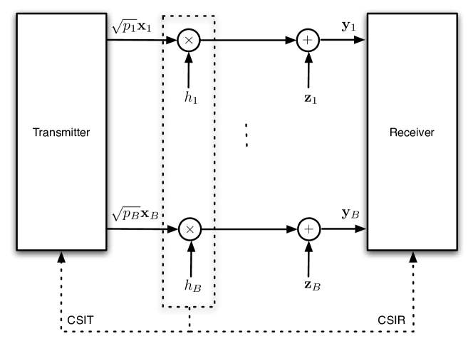
Figure 1: Block diagram corresponding to the channel system model with CSI at the transmitter and the receiver.

Consider transmission over an additive white Gaussian noise (AWGN) block-fading channel with $B$ blocks of $L$ channel uses each, in which, for $b=1,\ldots,B$, block $b$ is affected by a flat fading coefficient $h_{b}\in\mathbb{C}$. The corresponding block diagram is shown in Figure 1. Let $\gamma_{b}=|h_{b}|^{2}$ be the power fading gain and assume that the fading gain vector $\mbox{\boldmath{$\gamma$}}=(\gamma_{1},\ldots,\gamma_{B})$ is available at both the transmitter and the receiver. The transmit power is allocated to the blocks according to the scheme $\mathbf{p}(\mbox{\boldmath{$\gamma$}})=(p_{1}(\mbox{\boldmath{$\gamma$}}),\ldots,p_{B}(\mbox{\boldmath{$\gamma$}}))$. Then, the complex baseband channel model can be written as

$$\mathbf{y}_{b}=\sqrt{p_{b}(\mbox{\boldmath{$\gamma$}})}h_{b}\mathbf{x}_{b}+\mathbf{z}_{b},\ \ b=1,\ldots,B,$$ (1)

where $\mathbf{y}_{b}\in\mathbb{C}^{L}$ is the received signal in block $b$, $\mathbf{x}_{b}\in\mathcal{X}^{L}\subset\mathbb{C}^{L}$ is the portion of the codeword being transmitted in block $b$, $\mathcal{X}\subset\mathbb{C}$ is the signal constellation and $\mathbf{z}_{b}\in\mathbb{C}^{L}$ is a noise vector with independent, identically distributed (i.i.d.) circularly symmetric Gaussian entries $\sim\mathcal{N}_{\mathbb{C}}(0,1)$. Assume that the signal constellation $\mathcal{X}$ is normalized in energy such that $\sum_{x\in\mathcal{X}}|x|^{2}=2^{M}$, where $M=\log_{2}|\mathcal{X}|$. Then, the instantaneous received SNR at block $b$ is given by $p_{b}(\mbox{\boldmath{$\gamma$}})\gamma_{b}$. The following power constraints are considered [12]

Short-Term: $$\;\;\;\;\;\langle\mathbf{p}(\mbox{\boldmath{$\gamma$}})\rangle\triangleq\frac{1}{B}\sum_{b=1}^{B}p_{b}(\mbox{\boldmath{$\gamma$}})\leq P$$ (2)

Long-Term: $$\;\;\;\;\;\mathbb{E}\left[\langle\mathbf{p}(\mbox{\boldmath{$\gamma$}})\rangle\right]=\mathbb{E}\left[\frac{1}{B}\sum_{b=1}^{B}p_{b}(\mbox{\boldmath{$\gamma$}})\right]\leq P.$$ (3)

In all cases, $P$ represents the average SNR at the receiver. We will denote by $\mathbf{p}_{\rm st}$ and $\mathbf{p}_{\rm lt}$ the power allocation vectors corresponding to short- and long-term power constraints, respectively. We will also denote by $\mathbf{p}_{\rm eq}(p)=(p,\dotsc,p)$ the uniform power vector that allocates the same power $p$ to each block.

We consider block-fading channels where $h_{b}$ are independent realizations of a random variable $H$, whose magnitude is Nakagami-$m$ distributed [30, 31] and has a uniformly distributed phase. The fading magnitude has the following probability density function (pdf)

$$f_{|H|}(h)=\frac{2m^{m}h^{2m-1}}{\Gamma(m)}e^{-mh^{2}},$$ (4)

where $\Gamma(a)$ is the Gamma function, $\Gamma(a)=\int_{0}^{\infty}t^{a-1}e^{-t}dt$ [32]. The coefficients $\gamma_{b}$ are realizations of the random variable $|H|^{2}$ whose pdf and cdf are given by

$$f_{\gamma_{b}}(\gamma)=\begin{cases}\frac{m^{m}\gamma^{m-1}}{\Gamma(m)}e^{-m\gamma},&\gamma\geq 0\\ 0,&{\rm otherwise}\end{cases}$$ (5)

and

$$F_{\gamma_{b}}(\xi)=\begin{cases}1-\frac{\Gamma(m,m\xi)}{\Gamma(m)},&\xi\geq 0\\ 0,&{\rm otherwise},\end{cases}$$ (6)

respectively, where $\Gamma(a,\xi)$ is the upper incomplete Gamma function, $\Gamma(a,\xi)=\int_{\xi}^{\infty}t^{a-1}e^{-t}dt$ [32].

The Nakagami-$m$ distribution encompasses many fading distributions of interest. In particular, we obtain Rayleigh fading by letting $m=1$ and an accurate approximation of Rician fading with parameter $K$ by setting $m=(K+1)^{2}/(2K+1)$ [31].

III Mutual Information, MMSE and Outage Probability

The channel model described in (1) corresponds to a parallel channel model, where each sub-channel is used a fraction $\frac{1}{B}$ of the total number of channel uses per codeword. Therefore, for any given power fading gain realization $\gamma$ and power allocation scheme $\mathbf{p}(\mbox{\boldmath{$\gamma$}})$, the instantaneous input-output mutual information of the channel is given by [18]

$$I_{B}(\mathbf{p}(\mbox{\boldmath{$\gamma$}}),\mbox{\boldmath{$\gamma$}})=\frac{1}{B}\sum_{b=1}^{B}I_{\mathcal{X}}(p_{b}\gamma_{b}),$$ (7)

where $I_{\mathcal{X}}(\rho)$ is the input-output mutual information of an AWGN channel with input constellation ${\mathcal{X}}$ and received SNR $\rho$. In this paper we will consider coded modulation (CM) schemes with uniform input distribution, for which $I_{\mathcal{X}}(\rho)$ is given by

$$I_{\mathcal{X}}^{\rm CM}(\rho)=M-\frac{1}{2^{M}}\sum_{x\in\mathcal{X}}\mathbb{E}_{Z}\left[\log_{2}\left(\sum_{x^{\prime}\in\mathcal{X}}e^{-|\sqrt{\rho}(x-x^{\prime})+Z|^{2}+|Z|^{2}}\right)\right].$$

Furthermore, we also consider bit-interleaved coded modulation (BICM) using the classical sub-optimal non-iterative BICM decoder proposed in [33], for which the mutual information for a given binary labeling rule can be expressed as the mutual information of $M$ binary-input continuous-output-symmetric parallel channels [23],

$$I_{\mathcal{X}}^{\rm BICM}(\rho) =M-\frac{1}{2^{M}}\sum_{q=0}^{1}\sum_{j=1}^{M}\sum_{x\in\mathcal{X}_{q}^{j}}\mathbb{E}_{Z}\left[\log_{2}\frac{\displaystyle\sum_{x^{\prime}\in\mathcal{X}}e^{-|\sqrt{\rho}(X-x^{\prime})+Z|^{2}}}{\displaystyle\sum_{x^{\prime}\in\mathcal{X}_{q}^{j}}e^{-|\sqrt{\rho}(X-x^{\prime})+Z|^{2}}}\right].$$

where the sets $\mathcal{X}_{c}^{i}$ contain all signal constellation points with bit $c$ in the $j$-th binary labeling position. Both CM and BICM mutual information expressions can be efficiently evaluated numerically using Gauss-Hermite quadratures [32].

A fundamental relationship between the MMSE and the mutual information (in bits) in additive Gaussian channels is introduced in [22] showing that

$$\frac{d}{d\rho}I_{\mathcal{X}}(\rho)=\frac{1}{\log 2}{\rm MMSE}_{\mathcal{X}}(\rho),$$ (8)

where ${\rm MMSE}_{\mathcal{X}}(\rho)$ is the MMSE for a given signal constellation $\mathcal{X}$ expressed as a function of the SNR $\rho$. This relationship proves instrumental in obtaining optimal power control rules. In particular, for the CM case, the MMSE resulting from estimating the input based on the received signal over an AWGN channel with SNR $\rho$ can be written as [21],

$${\rm MMSE}_{\mathcal{X}}^{\rm CM}(\rho) =\mathbb{E}\left[|X-\hat{X}|^{2}\right]=\mathbb{E}\left[|X-\mathbb{E}\left[X|Y\right]|^{2}\right]$$ (9)

$$=1-\frac{1}{\pi}\int_{\mathbb{C}}\frac{\left|\sum_{x\in\mathcal{X}}xe^{-|y-\sqrt{\rho}x|^{2}}\right|^{2}}{\sum_{x\in\mathcal{X}}e^{-|y-\sqrt{\rho}x|^{2}}}dy,$$ (10)

where $\hat{X}=\mathbb{E}\left[X|Y\right]$ is the MMSE estimate of $X$ given the channel observation $Y$. Once again, (10) can be efficiently evaluated using Gauss-Hermite quadratures [32]. In the case of BICM, we obtain an equivalent set of symmetric binary-input continuous output channels [23]. However, due to the demodulation process, the equivalent channels have a noise that is non-Gaussian, and more importantly, non-additive. We therefore define the function derivative of $I_{\mathcal{X}}^{\rm BICM}(\rho)$, denoted by ${\rm MMSE}_{\mathcal{X}}^{\rm BICM}(\rho)$, by enforcing the relationship (8) to hold as follows

$${\rm MMSE}_{\mathcal{X}}^{\rm BICM}(\rho)\triangleq\frac{d}{d\rho}I_{\mathcal{X}}^{\rm BICM}(\rho).$$ (11)

Note that this is only a shorthand notation, so that whenever ${\rm MMSE}_{\mathcal{X}}$ appears in the coming sections, it can be replaced by either ${\rm MMSE}_{\mathcal{X}}^{\rm CM}(\rho)$ or ${\rm MMSE}_{\mathcal{X}}^{\rm BICM}(\rho)$. Therefore, (11) does not denote the MMSE in estimating the input bits given the noisy channel observation. The function ${\rm MMSE}_{\mathcal{X}}^{\rm BICM}(\rho)$ can again be easily evaluated numerically.

Finally, we define the transmission to be in outage when the instantaneous input-output mutual information is less than the target fixed transmission rate $R$. For a given power allocation scheme $\mathbf{p}(\mbox{\boldmath{$\gamma$}})$ with power constraint $P$, the outage probability at transmission rate $R$ is given by [6, 1]

$$P_{\rm out}(\mathbf{p}(\mbox{\boldmath{$\gamma$}}),P,R) =\Pr(I_{B}(\mathbf{p}(\mbox{\boldmath{$\gamma$}}),\mbox{\boldmath{$\gamma$}})<R)$$

$$=\Pr\left(\frac{1}{B}\sum_{b=1}^{B}I_{\mathcal{X}}(p_{b}\gamma_{b})<R\right).$$ (12)

Since $I_{\mathcal{X}}^{\rm BICM}(\rho)\leq I_{\mathcal{X}}^{\rm CM}(\rho)$ we will have that the corresponding outage probabilities verify that $P_{\rm out}^{\rm BICM}(\mathbf{p}(\mbox{\boldmath{$\gamma$}}),P,R)\geq P_{\rm out}^{\rm CM}(\mathbf{p}(\mbox{\boldmath{$\gamma$}}),P,R)$. All the algorithms and results presented in the following are valid for both CM and BICM. Therefore, unless explicitly stated, we will use the common notation $I_{\mathcal{X}}(\rho)$ and ${\rm MMSE}_{\mathcal{X}}(\rho)$ to refer to both.

IV Short-Term Power Allocation

Short-term power allocation schemes are applied to systems where the transmit power of each codeword is limited to $BP$. Following the definition of short-term power constraint given in Section II, a given short-term power allocation scheme $\mathbf{p}_{\rm st}=(p_{1},\ldots,p_{B})$ must then satisfy $\frac{1}{B}\sum_{b=1}^{B}p_{b}\leq P$.

IV-A Optimal Short-Term Power Allocation

The optimal short-term power allocation rule $\mathbf{p}^{\rm opt}_{\rm st}(\mbox{\boldmath{$\gamma$}})$ is the solution to the outage probability minimization problem [12]. Mathematically we express $\mathbf{p}^{\rm opt}_{\rm st}(\mbox{\boldmath{$\gamma$}})$ as

$$\mathbf{p}^{\rm opt}_{\rm st}(\mbox{\boldmath{$\gamma$}})=\arg\min_{\begin{subarray}{c}{\mathbf{p}}\in\mathbb{R}^{B}_{+}\\ \frac{1}{B}\sum_{b=1}^{B}p_{b}=P\end{subarray}}P_{\rm out}(\mathbf{p},P,R).$$ (13)

For short-term power allocation, the power allocation scheme that maximizes the instantaneous mutual information at each channel realization also minimizes the outage probability since the available power can only be distributed within one codeword. Formally, we have [12]

Lemma 1

Let $\mathbf{p}^{\rm opt}_{\rm st}(\mbox{\boldmath{$\gamma$}})$ be a solution of the problem

$$\begin{cases}\text{Maximize}&\sum_{b=1}^{B}I_{\mathcal{X}}(p_{b}\gamma_{b})\\ \text{Subject to}&\frac{1}{B}\sum_{b=1}^{B}p_{b}\leq P\\ &p_{b}\geq 0,b=1,\ldots,B.\end{cases}$$ (14)

Then $\mathbf{p}^{\rm opt}_{\rm st}(\mbox{\boldmath{$\gamma$}})$ is a solution of $\eqref{eq:opt_short_prob}$.

Proof:

See Appendix A. ∎

The solution of problem (14), which is based on the relationship between the MMSE and the mutual information [22], was obtained in [21]. From [21] one has the following theorem.

Theorem 1

The solution of problem (14) is given by

$$p^{\rm opt}_{b}(\mbox{\boldmath{$\gamma$}})=\frac{1}{\gamma_{b}}{\rm MMSE}_{\mathcal{X}}^{-1}\left(\min\left\{1,\frac{\eta}{\gamma_{b}}\right\}\right),$$ (15)

for $b=1,\dotsc,B$, where $\eta$ is chosen such that the power constraint is satisfied,

$$\frac{1}{B}\sum_{b=1}^{B}\frac{1}{\gamma_{b}}{\rm MMSE}_{\mathcal{X}}^{-1}\left(\min\left\{1,\frac{\eta}{\gamma_{b}}\right\}\right)=P.$$ (16)

Proof:

See [21] for details. ∎

As outlined in [21], the results of Theorem 1, are valid for any constellation. In particular, since the MMSE for Gaussian inputs (GI) is

$${\rm MMSE}_{\mathcal{X}}^{\rm GI}(\rho)=\frac{1}{\log 2\,(1+\rho)},$$ (17)

the inverse function can be written in closed form [21] and we therefore recover the waterfillng solution by replacing ${\rm MMSE}_{\mathcal{X}}(\rho)$ by ${\rm MMSE}_{\mathcal{X}}^{\rm GI}(\rho)$ [12].

The optimal short-term power allocation scheme improves the outage performance of coded modulation schemes over block-fading channels. However, it does not increase the outage diversity compared to a uniform power allocation, as shown in the following result.

Proposition 1

Consider transmission over the block-fading channel defined in (1) with the optimal power allocation scheme $\mathbf{p}_{\rm st}^{\rm opt}(\mbox{\boldmath{$\gamma$}})$ given in (15). Assume input constellation size $|\mathcal{X}|=2^{M}$. Further assume that the power fading gains follow the distribution given in (5). Then, for large $P$ and some $\mathcal{K}_{\rm opt}>0$ the outage probability behaves as

$$P_{\rm out}(\mathbf{p}_{\rm st}^{\rm opt}(\mbox{\boldmath{$\gamma$}}),P,R)\doteq\mathcal{K}_{\rm opt}P^{-md_{B}(R)},$$ (18)

where $d_{B}(R)$ is the Singleton bound given by

$$d_{B}(R)=1+\left\lfloor B\left(1-\frac{R}{M}\right)\right\rfloor.$$ (19)

Proof:

See Appendix A. ∎

IV-B Sub-optimal Short-Term Power Allocation Schemes

Although the power allocation scheme in (15) is optimal, it involves an inverse MMSE function, which may be excessively complex to implement or store for specific low-cost systems. Moreover, the MMSE function provides little insight into the role of each system parameter. In this section, we propose sub-optimal power allocation schemes similar to water-filling that tackle both drawbacks, leading to only minor losses in outage performance as compared to the optimal solution.

IV-B1 Truncated water-filling scheme

The complexity of the solution in (15) is due to the complex expression of $I_{\mathcal{X}}(\rho)$ in problem (14). Therefore, in order to obtain a simple sub-optimal solution, we propose an approximation for $I_{\mathcal{X}}(\rho)$ in problem (14). For Gaussian input channels with $I(\rho)=\log_{2}(1+\rho)$, optimal power allocation is obtained by the simple water-filling scheme [18]. This suggests the use of the following approximation for $I_{\mathcal{X}}(\rho)$.

$$I_{\mathcal{X}}(\rho)\leq I^{\rm tw}(\rho)\triangleq\begin{cases}\log_{2}(1+\rho),&\rho\leq\beta\\ \log_{2}(1+\beta),&\text{otherwise,}\end{cases}$$ (20)

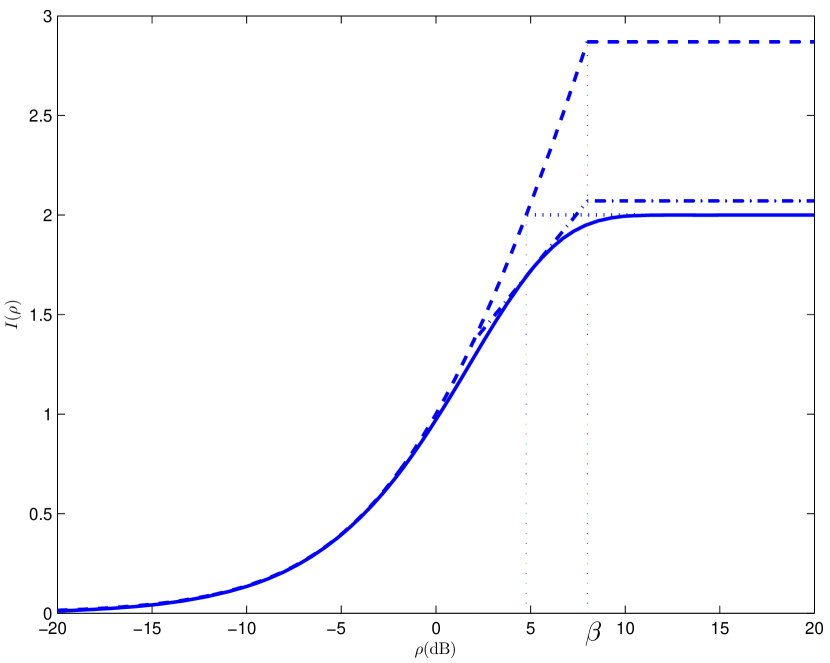
Figure 2: Mutual information of QPSK, and the approximations used by truncated water-filling and its corresponding refinement.

where $\beta$ is a design parameter to be optimized for best performance. An example of $I^{\rm tw}(\rho)$ is illustrated in Figure 2. The resulting sub-optimal scheme $\mathbf{p}_{\rm st}^{\rm tw}(\mbox{\boldmath{$\gamma$}})$ is given as a solution of

$$\begin{cases}\text{Maximize}&\sum_{b=1}^{B}I^{\rm tw}(p_{b}\gamma_{b})\\ \text{Subject to}&\frac{1}{B}\sum_{b=1}^{B}p_{b}\leq P\\ &p_{b}\geq 0,\ b=1,\ldots,B.\end{cases}$$ (21)

Theorem 2

A solution to the problem in (21) is given by

$$p^{\rm tw}_{b}(\mbox{\boldmath{$\gamma$}})=\begin{cases}\frac{\beta}{\gamma_{b}},&{\rm if}~{}\frac{1}{B}\sum_{b=1}^{B}\frac{\beta}{\gamma_{b}}\leq P\\ \min\left\{\frac{\beta}{\gamma_{b}},\left(\eta-\frac{1}{\gamma_{b}}\right)_{+}\right\},&\text{otherwise},\end{cases}$$ (22)

for $b=1,\ldots,B$, where $\eta$ is chosen such that

$$\frac{1}{B}\sum_{b=1}^{B}\min\left\{\frac{\beta}{\gamma_{b}},\left(\eta-\frac{1}{\gamma_{b}}\right)_{+}\right\}=P.$$ (23)

Proof:

See Appendix B. ∎

Without loss of generality, assume that $\gamma_{1}\geq\ldots\geq\gamma_{B}$, then, similarly to water-filling, $\eta$ can be determined such that [12]

$$(k-l)\eta=BP-\sum_{b=1}^{l}\frac{\beta+1}{\gamma_{b}}+\sum_{b=1}^{k}\frac{1}{\gamma_{b}},$$ (24)

where $k,l$ are integers satisfying $\frac{1}{\gamma_{k}}<\eta<\frac{1}{\gamma_{k+1}}$ and $\frac{\beta+1}{\gamma_{l}}<\eta\leq\frac{\beta+1}{\gamma_{l+1}}$.

From Theorem 2, the resulting power allocation scheme is similar to water-filling, except for the truncation of the allocated power at $\frac{\beta}{\gamma_{b}}$. We refer to this scheme as truncated water-filling. The outage performance obtained by the truncated water-filling scheme depends on the choice of the design parameter $\beta$. We now analyze the asymptotic performance of the outage probability, thus providing some guidance for the choice of $\beta$.

Proposition 2

Consider transmission over the block-fading channel defined in (1) with input constellation $\mathcal{X}$ and the truncated water-filling power allocation scheme $\mathbf{p}^{\rm tw}_{\rm st}(\mbox{\boldmath{$\gamma$}})$ given in (22). Assume that the power fading gains follow the distribution given in (5). Then, for large $P$, the outage probability $P_{\rm out}(\mathbf{p}^{\rm tw}_{\rm st}(\mbox{\boldmath{$\gamma$}}),P,R)$ is asymptotically upper bounded by

$$P_{\rm out}(\mathbf{p}^{\rm tw}_{\rm st}(\mbox{\boldmath{$\gamma$}}),P,R)~{}\dot{\leq}~{}\mathcal{K}_{\beta}P^{-md_{\beta}(R)},$$ (25)

where

$$d_{\beta}(R)=1+\left\lfloor B\left(1-\frac{R}{I_{\mathcal{X}}(\beta)}\right)\right\rfloor,$$ (26)

and $I_{\mathcal{X}}(\beta)$ is the input-output mutual information of an AWGN channel with SNR $\beta$.

Proof:

See Appendix C. ∎

From the results of Proposition 1, Proposition 2, and noting that $P_{\rm out}(\mathbf{p}^{\rm tw}_{\rm st}(\mbox{\boldmath{$\gamma$}}),P,R)\geq P_{\rm out}(\mathbf{p}^{\rm opt}_{\rm st}(\mbox{\boldmath{$\gamma$}}),P,R)$, we have

$$P_{\rm out}(\mathbf{p}^{\rm tw}_{\rm st}(\mbox{\boldmath{$\gamma$}}),P,R)\doteq\mathcal{K}_{\rm tw}P^{-md_{\rm tw}(R)},$$ (27)

where $d_{\rm tw}(R)$ satisfies that $d_{\beta}(R)\leq d_{\rm tw}(R)\leq d_{B}(R)$. Therefore, the truncated water-filling scheme is guaranteed to obtain optimal diversity whenever $d_{\beta}(R)=d_{B}(R)$, or equivalently, when

$$B\left(1-\frac{R}{I_{\mathcal{X}}(\beta)}\right) \geq\left\lfloor B\left(1-\frac{R}{M}\right)\right\rfloor$$ (28)

$$I_{\mathcal{X}}(\beta) \geq\frac{BR}{B-\left\lfloor B\left(1-\frac{R}{M}\right)\right\rfloor},$$ (29)

which implies that

$$\beta\geq I_{\mathcal{X}}^{-1}\left(\frac{BR}{B-\left\lfloor B\left(1-\frac{R}{M}\right)\right\rfloor}\right)\triangleq\beta_{R}.$$

Therefore, by letting $\beta\to\infty$, the truncated water-filling power allocation scheme given in (22), which now becomes the classical water-filling algorithm for Gaussian inputs, provides optimal outage diversity at any transmission rate. For any rate $R$ that is not at a discontinuity point of the Singleton bound, i.e. $R$ such that $B\left(1-\frac{R}{M}\right)$ is not an integer, we can always design a truncated water-filling scheme that obtains optimal diversity by choosing $\beta\geq\beta_{R}$.

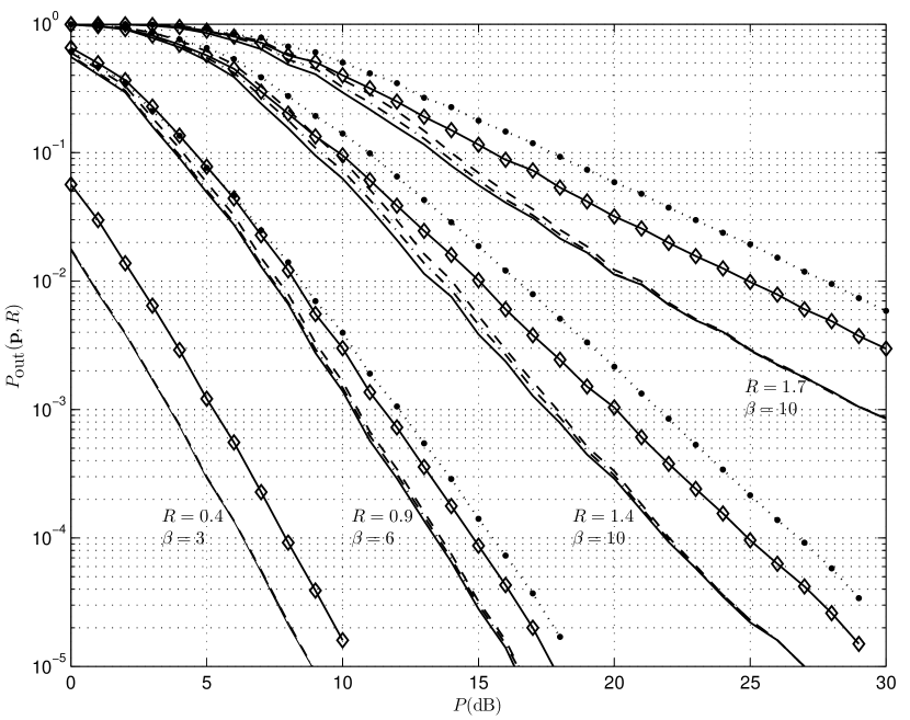
Figure 3: Outage performance of various short-term power allocation schemes for QPSK-input block-fading channels with $B=4$ and Rayleigh fading. The solid-lines represent the optimal scheme; the solid lines with $\diamond$ represent uniform power allocation; the dashed lines and dashed-dotted lines represent truncated water-filling and its corresponding refinement, respectively; the dotted lines represent the classical water-filling scheme.

With the results above, we choose $\beta$ as follows. For a transmission rate $R$ that is not a discontinuity point of the Singleton bound, we perform a simulation to compute the outage probability obtained by truncated water-filling with various $\beta\geq\beta_{R}$ and pick the $\beta$ that gives the best outage performance. The dashed lines in Figure 3 illustrate the performance of the obtained schemes for block-fading channels with $B=4$ and QPSK input under Rayleigh fading. At all rates of interest, the truncated water-filling schemes suffer only minor losses in outage performance as compared to the optimal schemes (solid lines), especially at high SNR. We also observe a remarkable difference with respect to pure water-filling for Gaussian inputs (dotted lines). As a matter of fact, pure water-filling performs worse than uniform power allocation.

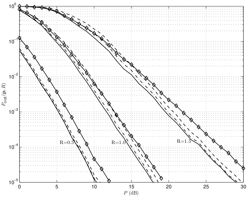
Figure 4: Outage performance of various short-term power allocation schemes for QPSK-input block-fading channels with $B=4$ and Rayleigh fading. The solid-lines represent the optimal scheme; the solid lines with $\diamond$ represent the uniform power allocation; the dashed lines and dashed-dotted lines correspondingly represent the truncated water-filling and its refinement with $\beta=15$.

For rates at the discontinuous points of the Singleton bound, especially when operating at high SNR, $\beta$ needs to be relatively large in order to maintain diversity. However, large $\beta$ increases the gap between $I^{\rm tw}(\rho)$ and $I_{\mathcal{X}}(\rho)$, thus degrading the performance of the truncated water-filling scheme. For $\beta=15$, the gap is illustrated by the dashed lines in Figure 4. In the extreme case where $\beta\to\infty$, the truncated water-filling turns into the water-filling scheme, which exhibits a significant loss in outage performance as illustrated in Figure 3.

IV-B2 Refined truncated water-filling schemes

To obtain a better approximation to the optimal power allocation scheme, we need a more accurate approximation to $I_{\mathcal{X}}(\rho)$ in (14). We propose the following bound.

$$I_{\mathcal{X}}(\rho)\leq I^{\rm ref}(\rho)\triangleq\begin{cases}\log_{2}(1+\rho),&\rho\leq\alpha\\ \kappa\log_{2}(\rho)+a,&\alpha<\rho\leq\beta\\ \kappa\log_{2}(\beta)+a,&\text{otherwise,}\end{cases}$$ (30)

where $\kappa$ and $a$ are chosen such that (in a dB scale) $\kappa\log_{2}(\rho)+a$ is a tangent to $I_{\mathcal{X}}(\rho)$ at a predetermined point $\rho_{0}$. Therefore $\alpha$ is chosen such that $\kappa\log_{2}(\alpha)+a=\log_{2}(1+\alpha)$, and $\beta$ is a design parameter. These parameters are reported in Table I for CM and BICM using various modulation schemes. An example of the approximation is also illustrated by the dashed-dotted curve in Figure 2.

The corresponding optimization problem can be written as

$$\begin{cases}\text{Maximize}&\sum_{b=1}^{B}I^{\rm ref}(p_{b}\gamma_{b})\\ \text{Subject to}&\sum_{b=1}^{B}p_{b}\leq BP\\ &p_{b}\geq 0,b=1,\ldots,B.\end{cases}$$ (31)

The refined truncated water-filling scheme $\mathbf{p}_{\rm st}^{\rm ref}(\mbox{\boldmath{$\gamma$}})$ is given by the following theorem.

Theorem 3

A solution to problem (31) is

$$p^{\rm ref}_{b}=\frac{\beta}{\gamma_{b}},\,\,\,b=1,\ldots,B$$ (32)

if $\frac{1}{B}\sum_{b=1}^{B}\frac{\beta}{\gamma_{b}}<P$, and otherwise,

$$p^{\rm ref}_{b}=\begin{cases}\frac{\beta}{\gamma_{b}},&\eta\geq\frac{\beta}{\kappa\gamma_{b}}\\ \kappa\eta,&\frac{\alpha}{\kappa\gamma_{b}}\leq\eta<\frac{\beta}{\kappa\gamma_{b}}\\ \frac{\alpha}{\gamma_{b}},&\frac{\alpha+1}{\gamma_{b}}\leq\eta<\frac{\alpha}{\kappa\gamma_{b}}\\ \eta-\frac{1}{\gamma_{b}},&\frac{1}{\gamma_{b}}\leq\eta<\frac{\alpha+1}{\gamma_{b}}\\ 0,&\text{otherwise,}\end{cases}$$ (33)

for $b=1,\ldots,B$, where $\eta$ is chosen such that

$$\frac{1}{B}\sum_{b=1}^{B}p^{\rm ref}_{b}=P.$$ (34)

Proof:

See Appendix D. ∎

The refined truncated water-filling scheme provides significant gain over the truncated water-filling scheme, especially when the transmission rate requires a relatively large $\beta$ to maintain the outage diversity. The dashed-dotted lines in Figure 4 show the outage performance of the refined truncated water-filling scheme for block-fading channels with $B=4$, and QPSK input under Rayleigh fading. The outage performance of the refined truncated water-filling scheme is close to the outage performance of the optimal case even at the rates where the Singleton bound is discontinuous, i.e. rates $R=0.5,1.0,1.5$. The performance gains of the refined scheme over the truncated water-filling scheme at other rates are also illustrated by the dashed-dotted lines in Figure 3.

V Long-Term Power Allocation

We consider systems with long-term power constraints, in which the expectation of the power allocated to each block (over infinitely many codewords) does not exceed $P$. This problem has been investigated in [12] for block-fading channels with Gaussian inputs. In this section, we obtain similar results for channels with discrete inputs, and propose sub-optimal schemes that reduce the complexity of the algorithm.

V-A Optimal Long-Term Power Allocation

Following [12], the problem can be formulated as

$$\begin{cases}\text{Minimize }&\Pr(I_{B}(\mathbf{p}_{\rm lt}(\mbox{\boldmath{$\gamma$}}),\mbox{\boldmath{$\gamma$}})<R)\\ \text{Subject to}&\mathbb{E}\left[\langle\mathbf{p}_{\rm lt}(\mbox{\boldmath{$\gamma$}})\rangle\right]\leq P,\\ \end{cases}$$ (35)

where $\langle\mathbf{p}\rangle=\frac{1}{B}\sum_{b=1}^{B}p_{b}$.

The following theorem shows that the structure of the optimal long-term solution $\mathbf{p^{\rm opt}_{\rm lt}}(\mbox{\boldmath{$\gamma$}})$ of [12] for Gaussian inputs is generalized to the discrete-input case.

Theorem 4

Consider transmission over the block-fading channel given in (1) with input constellation $\mathcal{X}$. Assume that the power fading gains in $\gamma$ follow the distribution given in (5). Then, the optimal power allocation scheme for systems with long-term constraint $P$, is given by

$$\mathbf{p^{\rm opt}_{\rm lt}}(\mbox{\boldmath{$\gamma$}})=\begin{cases}\mbox{\boldmath{$\wp$}}^{\rm opt}(\mbox{\boldmath{$\gamma$}}),&\langle\mbox{\boldmath{$\wp$}}^{\rm opt}(\mbox{\boldmath{$\gamma$}})\rangle\leq s\\ 0,&{\rm otherwise,}\end{cases}$$ (36)

where

1. $\mbox{\boldmath{$\wp$}}^{\rm opt}(\mbox{\boldmath{$\gamma$}})$ is the solution of the following optimization problem:

   $$\left\{\begin{array}[]{ll}{\rm Minimize}&\langle\mbox{\boldmath{$\wp$}}(\mbox{\boldmath{$\gamma$}})\rangle\\ {\rm Subject\ to}&\frac{1}{B}\sum_{b=1}^{B}I_{\mathcal{X}}(\wp_{b}\gamma_{b})\geq R\\ &\wp_{b}\geq 0,b=1,\ldots,B.\end{array}\right.$$ (37)

2. $s$ satisfies

   $$\left\{\begin{array}[]{lll}s&=\infty&$if$~{}\lim_{s\to\infty}\mathbb{E}_{\mathcal{R}(s)}\left[\langle\mbox{\boldmath{$\wp$}}^{\rm opt}(\mbox{\boldmath{$\gamma$}})\rangle\right]\leq P\\ P&=\mathbb{E}_{\mbox{\boldmath{$\gamma$}}\in\mathcal{R}(s)}\left[\langle\mbox{\boldmath{$\wp$}}^{\rm opt}(\mbox{\boldmath{$\gamma$}})\rangle\right],&{\rm otherwise,}\end{array}\right.$$ (38)

   in which,

   $$\mathcal{R}(s)\triangleq\left\{\mbox{\boldmath{$\gamma$}}\in\mathbb{R}_{+}^{B}:\langle\mbox{\boldmath{$\wp$}}^{\rm opt}(\mbox{\boldmath{$\gamma$}})\rangle\leq s\right\}.$$ (39)

Proof:

See Appendix E. ∎

Theorem 5

Consider transmission at rate $R$ over the block-fading channel given in (1) with input constellation $\mathcal{X}$ and realized power fading gain $\gamma$, the power allocation scheme that minimizes the input power, which is a solution of the problem given in (37), is given by

$$\wp_{b}^{\rm opt}(\mbox{\boldmath{$\gamma$}})=\frac{1}{\gamma_{b}}{\rm MMSE}_{\mathcal{X}}^{-1}\left(\min\left\{1,\frac{1}{\eta\gamma_{b}}\right\}\right),$$ (40)

where $\eta$ is chosen such that

$$\frac{1}{B}\sum_{\begin{subarray}{c}b=1\\ \gamma_{b}\geq\frac{1}{\eta}\end{subarray}}^{B}I_{\mathcal{X}}\left({\rm MMSE}_{\mathcal{X}}^{-1}\left(\frac{1}{\eta\gamma_{b}}\right)\right)=R.$$ (41)

Proof:

See Appendix F. ∎

As in the Gaussian input case [12], the optimal power allocation scheme either transmits with the minimum power that enables transmission at the target rate using an underlying dual short-term scheme $\mbox{\boldmath{$\wp$}}^{\rm opt}(\mbox{\boldmath{$\gamma$}})$ with short-term constraint $\langle\mbox{\boldmath{$\wp$}}^{\rm opt}(\mbox{\boldmath{$\gamma$}})\rangle<s$, or turns off transmission (allocating zero power) when the channel realization is bad. Therefore, there is no power wastage on outage events.

The solid lines in Figures 5 and 6 illustrate the outage performance of optimal long-term power allocation schemes for transmission over 4-block block-fading channels with QPSK and $16$-QAM inputs and Rayleigh fading ($m=1$). The simulation results suggest that for transmission rates where $d_{B}(R)>1$, zero outage probability can be obtained with finite power. This agrees with the results obtained for block-fading channels with Gaussian inputs [12], where only for $B>1$ zero outage is possible.

To provide more insight into this effect, consider the following long-term power allocation scheme,

$$\mathbf{p}_{\rm lt}(\mbox{\boldmath{$\gamma$}})=\begin{cases}\mbox{\boldmath{$\wp$}}(\mbox{\boldmath{$\gamma$}}),&\mbox{\boldmath{$\gamma$}}\in\mathcal{R}(s)\\ 0,&{\rm otherwise,}\end{cases}$$ (42)

where $\mbox{\boldmath{$\wp$}}(\mbox{\boldmath{$\gamma$}})$ is an arbitrary underlying short-term power allocation scheme,

$$\mathcal{R}(s)=\left\{\mbox{\boldmath{$\gamma$}}\in\mathbb{R}_{+}^{B}:\langle\mbox{\boldmath{$\wp$}}(\mbox{\boldmath{$\gamma$}})\rangle\leq s\right\},$$ (43)

and $s$ is chosen to satisfy the long-term power constraint,

$$\mathbb{E}\left[\langle\mathbf{p}_{\rm lt}(\mbox{\boldmath{$\gamma$}})\rangle\right]=\mathbb{E}_{\mbox{\boldmath{$\gamma$}}\in\mathcal{R}(s)}\left[\langle\mbox{\boldmath{$\wp$}}(\mbox{\boldmath{$\gamma$}})\rangle\right]=P.$$ (44)

Assuming that for any $s$, $\mbox{\boldmath{$\wp$}}(\mbox{\boldmath{$\gamma$}})$ satisfies $\frac{1}{B}\sum_{b=1}^{B}I_{\mathcal{X}}(\wp_{b}\gamma_{b})\geq R$ for any $\mbox{\boldmath{$\gamma$}}\in\mathcal{R}(s)$, then the resulting outage probability of the corresponding long-term power allocation is

$$P_{\rm out}(\mathbf{p}_{\rm lt}(\mbox{\boldmath{$\gamma$}}),P(s),R)=\Pr(\mbox{\boldmath{$\gamma$}}\notin\mathcal{R}(s)).$$ (45)

For any long-term power constraint $P$, the long-term power allocation scheme in (42) depends on the threshold $s$ defined in (44). Conversely, for any choice of the threshold $s$, the long-term power $P(s)$ is given by

$$P(s)=\mathbb{E}_{\mbox{\boldmath{$\gamma$}}\in\mathcal{R}(s)}\left[\langle\mbox{\boldmath{$\wp$}}(\mbox{\boldmath{$\gamma$}})\rangle\right].$$ (46)

We now consider the behavior of the average power $P(s)$ and the corresponding outage probability $P_{\rm out}(\mathbf{p}_{\rm lt}(\mbox{\boldmath{$\gamma$}}),P(s),R)$ when $s\to\infty$. In particular, we study the long-term exponent defined as

$$d_{\rm lt}(R)\triangleq\lim_{P(s)\to\infty}-\frac{\log P_{\rm out}(\mathbf{p}_{\rm lt}(\mbox{\boldmath{$\gamma$}}),P(s),R)}{\log P(s)}.$$ (47)

Firstly, consider the following asymptotic relationship between $s$ and $P(s)$.

Proposition 3

Consider transmission over a block-fading channel with a long-term power allocation scheme corresponding to an arbitrary underlying short-term scheme $\mbox{\boldmath{$\wp$}}(\mbox{\boldmath{$\gamma$}})$, a threshold $s$ given in (42), and a long-term power constraint $P(s)$ given in (46). Assume that $\mbox{\boldmath{$\wp$}}(\mbox{\boldmath{$\gamma$}})$ is chosen such that asymptotically in $s$, the outage probability satisfies

$$P_{\rm out}(\mathbf{p}_{\rm lt}(\mbox{\boldmath{$\gamma$}}),P(s),R)\doteq\mathcal{K}s^{-d(R)}$$ (48)

for some finite $d(R)>0$. Then,

$$\frac{d}{ds}P(s)\doteq\mathcal{K}d(R)s^{-d(R)}$$ (49)

Proof:

See Appendix G. ∎

From the previous proposition, we obtain the following result.

Theorem 6

Consider transmission over a block-fading channel with a long-term power allocation scheme corresponding to an arbitrary underlying short-term scheme $\mbox{\boldmath{$\wp$}}(\mbox{\boldmath{$\gamma$}})$, a threshold $s$ given in (42), and a long-term power constraint $P(s)$ given in (46). Assume that $\mbox{\boldmath{$\wp$}}(\mbox{\boldmath{$\gamma$}})$ is chosen such that asymptotically in $s$, the outage probability satisfies

$$P_{\rm out}(\mathbf{p}_{\rm lt}(\mbox{\boldmath{$\gamma$}}),P(s),R)\doteq\mathcal{K}s^{-d(R)}$$ (50)

for some finite $d(R)>0$. Then, if $d(R)>1$ we have that

$$\lim_{s\to\infty}P(s)=P_{\rm th}<\infty\,\,\,\,\text{and}\,\,\,\,d_{\rm lt}(R)=\infty,$$

while if $d(R)<1$,

$$d_{\rm lt}(R)=\frac{d(R)}{1-d(R)}.$$ (51)

Proof:

See Appendix G. ∎

The previous results highlight the effect of the power constraint on the outage performance obtained by a specific power allocation scheme $\mathbf{p}_{\rm lt}(\mbox{\boldmath{$\gamma$}})$. In particular, $P_{\rm out}(\mathbf{p}_{\rm lt}(\mbox{\boldmath{$\gamma$}}),P(s),R)$ is the outage probability of the block-fading channel with power allocation scheme $\mbox{\boldmath{$\wp$}}(\mbox{\boldmath{$\gamma$}})$ and short-term power constraint $\langle\mbox{\boldmath{$\wp$}}(\mbox{\boldmath{$\gamma$}})\rangle<s$, and $d(R)$ is the corresponding short-term outage diversity. When a long-term power constraint is applied, the long-term outage diversity $d_{\rm lt}(R)$ is affected in the following way:

• If $d(R)>1$, then $d_{\rm lt}(R)=\infty$ and $\lim_{s\to\infty}P(s)=P_{\rm th}<\infty$. Therefore, since

  $$\lim_{s\to\infty}P_{\rm out}(\mathbf{p}_{\rm lt}(\mbox{\boldmath{$\gamma$}}),P(s),R)=0,$$ (52)

  there exists a threshold long-term power constraint $P_{\rm th}$ beyond which strictly zero outage probability is achieved, proving that vanishing error probability can be achieved and that reliable communication is possible at rates below $R$. $R$ is therefore a lower bound to the delay limited capacity [13] of the block-fading channel with power constraint $P_{\rm th}$.

• If $d(R)<1$, then (51) gives the relationship between the long- and short-term outage diversity.

In order to apply the previous theorem to analyze the asymptotic behaviour of the optimal power allocation for systems with long-term constraints, we consider the following duality between $\mathbf{p}_{\rm st}^{\rm opt}(\mbox{\boldmath{$\gamma$}})$ and $\mbox{\boldmath{$\wp$}}^{\rm opt}(\mbox{\boldmath{$\gamma$}})$.

Proposition 4

Consider transmission at rate $R$ over the block-fading channel given in (1) with the optimal long-term power allocation scheme $\mathbf{p^{\rm opt}_{\rm lt}}(\mbox{\boldmath{$\gamma$}})$ given in (36) and a long-term power constraint $P(s)$. Then, independent of the fading statistics, the outage probability satisfies

$$P_{\rm out}(\mathbf{p}_{\rm lt}^{\rm opt}(\mbox{\boldmath{$\gamma$}}),P(s),R)=P_{\rm out}(\mathbf{p}_{\rm st}^{\rm opt}(\mbox{\boldmath{$\gamma$}}),s,R),$$ (53)

where $\mathbf{p}_{\rm st}^{\rm opt}(\mbox{\boldmath{$\gamma$}})$ is the optimal power allocation scheme with short-term power constraint $\langle\mathbf{p}_{\rm st}^{\rm opt}(\mbox{\boldmath{$\gamma$}})\rangle\leq s$.

Proof:

See Appendix G. ∎

From Theorem 6, we have the following result.

Corollary 1

Consider transmission at rate $R$ over the block-fading channel given in (1) with the optimal long-term power allocation scheme $\mathbf{p^{\rm opt}_{\rm lt}}(\mbox{\boldmath{$\gamma$}})$. Assume input constellation $\mathcal{X}$ of size $|\mathcal{X}|=2^{M}$. Further assume that the power fading gain $\gamma$ follows a Nakagami-$m$ distribution given in (5). Then, the delay-limited capacity is non-zero whenever $d_{B}(R)>\frac{1}{m}$. Conversely, when $d_{B}(R)<\frac{1}{m}$, the outage probability asymptotically behaves as

$$P_{\rm out}^{\rm lt}(\mathbf{p^{\rm opt}_{\rm lt}}(\mbox{\boldmath{$\gamma$}}),P(s),R)\doteq\mathcal{K}_{\rm lt}^{\rm opt}P^{-d_{\rm lt}^{\rm opt}(R)},$$ (54)

where $P$ is the long-term power constraint, and $d_{\rm lt}^{\rm opt}(R)$ is the optimal long-term outage diversity given by

$$d_{\rm lt}^{\rm opt}(R)=\frac{md_{B}(R)}{1-md_{B}(R)}.$$ (55)

Proof:

From Propositions 1 and 4, we have

$$P_{\rm out}^{\rm lt}(\mathbf{p^{\rm opt}_{\rm lt}}(\mbox{\boldmath{$\gamma$}}),P(s),R)\doteq\mathcal{K}_{\rm opt}s^{-md_{B}(R)}.$$ (56)

Therefore, the corollary can be obtained as a direct application of Theorem 6. ∎

This behavior is illustrated in Figure 7, where the outage probability with QPSK inputs, $m=0.5$ and $R=1.7$ has been plotted as a function of the average long-term power $P(s)$ and as a function of the dual short-term constraint $s$. As predicted by the previous results, the dual short-term curve has slope $md_{B}(R)=0.5$. Furthermore, since $d_{B}(R)=1<\frac{1}{m}=2$, we observe that the long-term outage curve (as a function of $P(s)$) has slope $d_{\rm lt}^{\rm opt}(R)=\frac{md_{B}(R)}{1-md_{B}(R)}=1$.

V-B Sub-optimal Long-Term Power Allocation

In the optimal long-term power allocation scheme $\mathbf{p}_{\rm lt}^{\rm opt}(\mbox{\boldmath{$\gamma$}})$ given in Theorem 4, $s$ can be evaluated offline for any fading distribution. Therefore, given an allocation scheme $\mbox{\boldmath{$\wp$}}^{\rm opt}(\mbox{\boldmath{$\gamma$}})$, the complexity required to evaluate $\mathbf{p}_{\rm lt}^{\rm opt}(\mbox{\boldmath{$\gamma$}})$ is low. Thus, the complexity of the long-term power allocation scheme is mainly due to the complexity of evaluating $\mbox{\boldmath{$\wp$}}^{\rm opt}(\mbox{\boldmath{$\gamma$}})$, which requires the evaluation or storage of ${\rm MMSE}_{\mathcal{X}}(\rho)$ and $I_{\mathcal{X}}(\rho)$. In this section, we propose sub-optimal long-term power allocation schemes by replacing the optimal underlying short-term algorithm $\mbox{\boldmath{$\wp$}}^{\rm opt}(\mbox{\boldmath{$\gamma$}})$ with simpler allocation rules.

A long-term power allocation scheme $\mathbf{p}_{\rm lt}(\mbox{\boldmath{$\gamma$}})$ corresponding to an arbitrary $\mbox{\boldmath{$\wp$}}(\mbox{\boldmath{$\gamma$}})$ is obtained by replacing $\mbox{\boldmath{$\wp$}}^{\rm opt}(\mbox{\boldmath{$\gamma$}})$ in (36), (38) and (39) with $\mbox{\boldmath{$\wp$}}(\mbox{\boldmath{$\gamma$}})$. From (36), the long-term power allocation scheme $\mathbf{p}_{\rm lt}(\mbox{\boldmath{$\gamma$}})$ satisfies

$$\mathbb{E}\left[\langle\mathbf{p}_{\rm lt}(\mbox{\boldmath{$\gamma$}})\rangle\right]= \mathbb{E}_{\mbox{\boldmath{$\gamma$}}\in\mathcal{R}(s)}\left[\langle\mbox{\boldmath{$\wp$}}(\mbox{\boldmath{$\gamma$}})\rangle\right]=P.$$ (57)

Therefore, a long-term power allocation scheme corresponding to an arbitrary $\mbox{\boldmath{$\wp$}}(\mbox{\boldmath{$\gamma$}})$ is sub-optimal with respect to $\mathbf{p}_{\rm lt}^{\rm opt}(\mbox{\boldmath{$\gamma$}})$. Following the transmission strategy in the optimal scheme, we consider the power allocation schemes $\mbox{\boldmath{$\wp$}}(\mbox{\boldmath{$\gamma$}})$ that satisfy the rate constraint $I_{B}(\mbox{\boldmath{$\wp$}}(\mbox{\boldmath{$\gamma$}}),\mbox{\boldmath{$\gamma$}})\geq R$ to avoid wasting power on outage events. These schemes are sub-optimal solutions of problem (37). Based on the short-term schemes, two simple rules are discussed in the next subsections.

V-B1 Long-term truncated water-filling scheme

Similar to the short-term truncated water-filling scheme, we consider approximating $I_{\mathcal{X}}(\rho)$ in (37) by $I^{\rm tw}(\rho)$ in (20), which results in the following problem

$$\begin{cases}\text{Minimize}&\langle\mbox{\boldmath{$\wp$}}(\gamma)\rangle\\ \text{Subject \ to \ }&\frac{1}{B}\sum_{b=1}^{B}I^{\rm tw}(\wp_{b}\gamma_{b})\geq R\\ &\wp_{b}\geq 0,b=1,\ldots,B\end{cases}$$ (58)

Theorem 7

Problem (58) is solved by $\mbox{\boldmath{$\wp$}}(\mbox{\boldmath{$\gamma$}})$ given as

$$\wp_{b}=\min\left\{\frac{\beta}{\gamma_{b}},\left(\eta-\frac{1}{\gamma_{b}}\right)_{+}\right\},b=1,\ldots,B,$$ (59)

where $\eta$ is chosen such that

$$\frac{1}{B}\sum_{b=1}^{B}\log_{2}(1+\wp_{b}\gamma_{b})=R.$$ (60)

Proof:

See Appendix H. ∎

Note that since $I^{\rm tw}(\rho)$ is an upper bound on $I_{\mathcal{X}}(\rho)$, $\mbox{\boldmath{$\wp$}}(\mbox{\boldmath{$\gamma$}})$ does not satisfy the rate constraint $I_{B}(\mbox{\boldmath{$\wp$}}(\mbox{\boldmath{$\gamma$}}),\mbox{\boldmath{$\gamma$}})\geq R$. By adjusting $\eta$, we can obtain a sub-optimal $\mbox{\boldmath{$\wp$}}^{\rm tw}(\mbox{\boldmath{$\gamma$}})$ as follows

$$\wp^{\rm tw}_{b}=\min\left\{\frac{\beta}{\gamma_{b}},\left(\eta-\frac{1}{\gamma_{b}}\right)_{+}\right\},b=1,\ldots,B,$$ (61)

where now $\eta$ is chosen according to the true mutual information with discrete inputs, namely, we choose $\eta$ such that

$$\frac{1}{B}\sum_{b=1}^{B}I_{\mathcal{X}}(\wp^{\rm tw}_{b}\gamma_{b})=R.$$ (62)

Using this scheme, we obtain a power allocation $\mathbf{p}_{\rm lt}^{\rm tw}(\mbox{\boldmath{$\gamma$}})$, which is the long-term power allocation scheme corresponding to the sub-optimal $\mbox{\boldmath{$\wp$}}^{\rm tw}(\mbox{\boldmath{$\gamma$}})$ of $\mbox{\boldmath{$\wp$}}^{\rm opt}(\mbox{\boldmath{$\gamma$}})$. The performance of the scheme is illustrated by the dashed lines in Figures 5 and 6. As we observe, the performance of the truncated water-filling scheme is very close to that of the optimal scheme.

Similar to the optimal power allocation scheme, we have the following duality between $\mathbf{p}_{\rm st}^{\rm tw}(\mbox{\boldmath{$\gamma$}})$ and $\mbox{\boldmath{$\wp$}}^{\rm tw}(\mbox{\boldmath{$\gamma$}})$.

Proposition 5

Consider transmission at rate $R$ over the block-fading channel given in (1) with power allocation scheme $\mathbf{p}_{\rm lt}^{\rm tw}(\mbox{\boldmath{$\gamma$}})$ and long-term power constraint $P(s)$. Then, independent of the fading statistics, the outage probability satisfies

$$P_{\rm out}(\mathbf{p}_{\rm lt}^{\rm tw},P(s),R)=P_{\rm out}(\mathbf{p}_{\rm st}^{\rm tw}(\mbox{\boldmath{$\gamma$}}),s,R),$$ (63)

where $\mathbf{p}_{\rm st}^{\rm tw}(\mbox{\boldmath{$\gamma$}})$ is the truncated water-filling power allocation scheme with short-term constraint $\langle\mathbf{p}_{\rm st}^{\rm tw}(\mbox{\boldmath{$\gamma$}})\rangle\leq s$.

Proof:

See Appendix I ∎

Therefore, from Theorem 6 and Lemma 2, we have the following result.

Corollary 2

Let $\mathbf{p}_{\rm lt}^{\rm tw}(\mbox{\boldmath{$\gamma$}})$ be the long-term power allocation scheme corresponding to $\mbox{\boldmath{$\wp$}}^{\rm tw}(\mbox{\boldmath{$\gamma$}})$ given in (61). Consider transmission at rate $R$ over the block-fading channel given in (1) with the long-term power allocation scheme $\mathbf{p}_{\rm lt}^{\rm tw}(\mbox{\boldmath{$\gamma$}})$. Assume that the power fading gain $\gamma$ follows a Nakagami-$m$ distribution given in (5). Then, the corresponding delay-limited capacity is non-zero if $d_{\beta}(R)>\frac{1}{m}$, where

$$d_{\beta}(R)=1+\left\lfloor B\left(1-\frac{R}{I_{\mathcal{X}}(\beta)}\right)\right\rfloor.$$ (64)

Proof:

From Propositions 5 and 2, we have

$$P_{\rm out}(\mathbf{p}_{\rm lt}^{\rm tw}(\mbox{\boldmath{$\gamma$}}),P(s),R)\doteq\mathcal{K}_{\rm tw}s^{-d_{\rm tw}(R)},$$ (65)

where $d_{\rm tw}(R)\geq d_{\beta}(R)$. Therefore, the proof follows as a result of Theorem 6. ∎

In Figure 7 we also show in dashed lines the corresponding long-term truncated water-filling outage curves, and we observe the same asymptotic behavior as for the optimal scheme.

V-B2 Refinement of the long-term truncated water-filling scheme

In order to improve the performance of the sub-optimal scheme, we approximate $I_{\mathcal{X}}(\rho)$ by $I^{\rm ref}(\rho)$ given in (30). Replacing $I_{\mathcal{X}}(\rho)$ in (37) by $I^{\rm ref}(\rho)$, we have the following problem

$$\begin{cases}\text{Minimize}&\langle\mbox{\boldmath{$\wp$}}(\gamma)\rangle\\ \text{Subject \ to \ }&\frac{1}{B}\sum_{b=1}^{B}I^{\rm ref}(\wp_{b}\gamma_{b})\geq R\\ &\wp_{b}\geq 0,b=1,\ldots,B.\end{cases}$$ (66)

Theorem 8

The problem given in (66) is solved by $\mbox{\boldmath{$\wp$}}(\mbox{\boldmath{$\gamma$}})$ given as

$$\wp_{b}=\begin{cases}\frac{\beta}{\gamma_{b}},&\eta\geq\frac{\beta}{\kappa\gamma_{b}}\\ \kappa\eta,&\frac{\alpha}{\kappa\gamma_{b}}<\eta<\frac{\beta}{\kappa\gamma_{b}}\\ \frac{\alpha}{\gamma_{b}},&\frac{\alpha+1}{\gamma_{b}}\leq\eta\leq\frac{\alpha}{\kappa\gamma_{b}}\\ \eta-\frac{1}{\gamma_{b}},&\frac{1}{\gamma_{b}}\leq\eta<\frac{\alpha+1}{\gamma_{b}}\\ 0,&{\rm otherwise,}\end{cases}$$ (67)

where $\eta$ is chosen such that

$$\sum_{b=1}^{B}I^{\rm ref}(\wp_{b}\gamma_{b})=BR.$$ (68)

Proof:

See Appendix J. ∎

Following the arguments in Section V-B1, we obtain the sub-optimal $\mbox{\boldmath{$\wp$}}^{\rm ref}(\mbox{\boldmath{$\gamma$}})$ of $\mbox{\boldmath{$\wp$}}^{\rm opt}(\mbox{\boldmath{$\gamma$}})$ from (67) by choosing $\eta$ in such that

$$\frac{1}{B}\sum_{b=1}^{B}I_{\mathcal{X}}(\wp^{\rm ref}_{b}\gamma_{b})=R.$$ (69)

The performance of the long-term power allocation corresponding to $\mbox{\boldmath{$\wp$}}^{\rm ref}(\mbox{\boldmath{$\gamma$}})$, $\mathbf{p}_{\rm lt}^{\rm ref}(\mbox{\boldmath{$\gamma$}})$, is illustrated by the dashed-dotted lines in Figures 5 and 6. We observe that refined truncated water-filling leads to performance closer to that of the optimal schemes than truncated water-filling. The improvements are particularly clear for higher transmission rates.

V-B3 Approximation of $I_{\mathcal{X}}(\rho)$

The sub-optimal schemes in the previous sections are significantly less complex than the corresponding optimal schemes, while only suffering minor losses in outage performance. However, the sub-optimal schemes still require the computation or storage of $I_{\mathcal{X}}(\rho)$ for determining $\eta$. This can be avoided by using an approximation of $I_{\mathcal{X}}(\rho)$. Let $\tilde{I}_{\mathcal{X}}(\rho)$ be an approximation of $I_{\mathcal{X}}(\rho)$ and $\Delta R$ be the error measure given by

$$\Delta R=\max_{\rho}\left\{\tilde{I}_{\mathcal{X}}(\rho)-I_{\mathcal{X}}(\rho)\right\}.$$ (70)

Then, for a sub-optimal scheme $\mbox{\boldmath{$\wp$}}(\mbox{\boldmath{$\gamma$}})$, $\eta$ is chosen such that

$$\sum_{b=1}^{B}\tilde{I}_{\mathcal{X}}(\wp_{b}\gamma_{b})=B(R+\Delta R)$$ (71)

satisfies the rate constraint since

$$\sum_{b=1}^{B}I_{\mathcal{X}}(\wp_{b}\gamma_{b})\geq\sum_{b=1}^{B}\tilde{I}_{\mathcal{X}}(\wp_{b}\gamma_{b})-B\Delta R=BR.$$ (72)

Following [35], we propose the following approximation for $I_{\mathcal{X}}(\rho)$

$$\tilde{I}_{\mathcal{X}}(\rho)=M\left(1-e^{-c_{1}\rho^{c_{2}}}\right)^{c_{3}}.$$ (73)

For channels with QPSK input, using numerical optimization to minimize the mean-squared-error between $I_{\mathcal{X}}(\rho)$ and $\tilde{I}_{\mathcal{X}}(\rho)$, we obtain the parameters, $c_{1},c_{2},c_{3}$, shown in Table II. Using this approximation to evaluate $\eta$ in subsections V-B1 and V-B2, we arrive at computationally efficient power allocation schemes with little loss in outage performance.

In Figure 8, we illustrate the significant gains achievable by the long-term schemes when compared to short-term schemes. As observed in [12], remarkable gains of $11$ dB at an outage probability of $10^{-4}$ are possible with optimal long-term power allocation when compared to uniform power allocation for Gaussian input distributions. As shown in Figure 8, similar gains of the order of $12$ dB at an outage probability of $10^{-4}$ are also achievable with discrete inputs. Note that, due to the Singleton bound, the slope of the QPSK-input short-term curves is not as steep as the slope of the corresponding Gaussian input or $16$-QAM input curves. This is due to the fact that both Gaussian and $16$-QAM inputs have SNR exponent $d(R)=4$ while QPSK has $d_{B}(R)=3$. Figure 9 shows similar results comparing CM and BICM. In particular, the figure shows little loss between the corresponding power allocation schemes. This is due to the fact that the mutual information curves from CM and BICM with Gray mapping do not differ much [23]. Once again, in the case of BICM, the loss incurred by suboptimal schemes is negligible.

We finally illustrate the application of the above results to practical OFDM channels. In particular, we show in Figure 10 the results corresponding to an OFDM channel with $B=64$ sub-carriers, whose $9$-tap symbol-period-sampled power delay profile is extracted from the ETSI BRAN-A model [36] using a zero-hold order filter. The power delay profile models a typical non-line-of-sight (NLOS) indoor office scenario and is given in Table III. We observe a similar behavior as in the block-fading channel. In particular, we show that in practical OFDM scenarios impressive gains of more than $10$ dB with respect to uniform power allocation (eventually reducing all outages) are possible. Note that due to the large frequency diversity induced by the time-domain channel in Table III, the uniform and short-term power allocation curves do not reveal their respective asymptotic slopes in the error probability range shown in the figure.

VI Conclusions

We considered power allocation schemes for fixed-rate transmission over discrete-input block-fading channels with transmitter and receiver CSI under short- and long-term power constraints. We have studied optimal and low-complexity sub-optimal schemes. In particular, we have analyzed the optimal diversity orders and we have shown that, in the long-term case, outages can be removed provided that the short-term SNR exponent be greater than one. We have illustrated the corresponding performances, showing significant performance advantages on the order of $10$ dB of the proposed long-term schemes when compared to uniform power allocation. Furthermore, we have shown that minimal loss is incurred when using the suggested sub-optimal schemes. We have also illustrated the applicability and performance advantages of the proposed techniques to practical OFDM situations.

Appendix A Optimal Power Allocation for Short-term Constraints

Proof of Lemma 1

Since $\mathbf{p}^{\rm opt}_{\rm st}(\mbox{\boldmath{$\gamma$}})$ is the solution of (14), we have

$$\sum_{b=1}^{B}I_{\mathcal{X}}(p^{\rm opt}_{b}\gamma_{b})\geq\sum_{b=1}^{B}I_{\mathcal{X}}(p_{b}\gamma_{b})$$ (74)

for any power allocation scheme $\mathbf{p}_{\rm st}(\mbox{\boldmath{$\gamma$}})$ satisfying the short-term power constraint. Therefore,

$$\Pr\left(\sum_{b=1}^{B}I_{\mathcal{X}}(p^{\rm opt}_{b}\gamma_{b})<BR\right)\leq\Pr\left(\sum_{b=1}^{B}I_{\mathcal{X}}(p_{b}\gamma_{b})<BR\right),$$ (75)

and thus,

$$P_{\rm out}(\mathbf{p}^{\rm opt}_{\rm st}(\mbox{\boldmath{$\gamma$}}),P,R)\leq P_{\rm out}(\mathbf{p}_{b}(\mbox{\boldmath{$\gamma$}}),P,R)$$ (76)

for any scheme $\mathbf{p}_{\rm st}(\mbox{\boldmath{$\gamma$}})$ satisfying the short-term power constraint. This proves that $\mathbf{p}^{\rm opt}_{\rm st}(\mbox{\boldmath{$\gamma$}})$ is a solution of (13).

Proof of Proposition 1

With the optimal power allocation scheme $\mathbf{p}^{\rm opt}_{\rm st}(\mbox{\boldmath{$\gamma$}})$, the outage probability is given by

$$P_{\rm out}(\mathbf{p}^{\rm opt}_{\rm st}(\mbox{\boldmath{$\gamma$}}),P,R)=\Pr\left(\frac{1}{B}\sum_{b=1}^{B}I_{\mathcal{X}}(p^{\rm opt}_{b}\gamma_{b})<R\right).$$ (77)

Since $\mathbf{p}^{\rm opt}_{\rm st}(\mbox{\boldmath{$\gamma$}})$ is the solution of (14), we have $p^{\rm opt}_{b}\geq 0,b=1,\ldots,B$ and $\frac{1}{B}\sum_{b=1}^{B}p^{\rm opt}_{b}\leq P$. Therefore, $0\leq p^{\rm opt}_{b}\leq BP,b=1,\ldots,B$. Thus, $P_{\rm out}(\mathbf{p}^{\rm opt}_{\rm st}(\mbox{\boldmath{$\gamma$}}),P,R)$ is lower bounded by

$$P_{\rm out}(\mathbf{p}^{\rm opt}_{\rm st}(\mbox{\boldmath{$\gamma$}}),P,R) \geq\Pr\left(\frac{1}{B}\sum_{b=1}^{B}I_{\mathcal{X}}(BP\gamma_{b})<R\right)$$ (78)

$$=P_{\rm out}(\mathbf{p}_{\rm eq}(BP),PB,R),$$ (79)

namely, the outage probability of block-fading channels corresponding to an equal allocation of power $PB$ per block. Now, according to [27], under Nakagami-$m$ fading statistics, we have that

$$P_{\rm out}(\mathbf{p}^{\rm opt}_{\rm st}(\mbox{\boldmath{$\gamma$}}),P,R) ~{}\dot{\geq}~{}\mathcal{K}(BP)^{-md_{B}(R)}$$ (80)

$$=\mathcal{K}B^{-md_{B}(R)}P^{-md_{B}(R)}.$$ (81)

Conversely, since the power allocation scheme is optimal, the outage performance is upper bounded by the allocation scheme that assigns power $P$ to each block. Therefore,

$$P_{\rm out}(\mathbf{p}^{\rm opt}_{\rm st}(\mbox{\boldmath{$\gamma$}}),P,R) \leq P_{\rm out}(\mathbf{p}_{\rm eq}(P),P,R)$$ (82)

$$\doteq\mathcal{K}P^{-md_{B}(R)}.$$ (83)

From (81) and (83), we have

$$P_{\rm out}(\mathbf{p}^{\rm opt}_{\rm st}(\mbox{\boldmath{$\gamma$}}),P,R)\doteq\mathcal{K}_{\rm opt}P^{-md_{B}(R)}.$$ (84)

Thus, the diversity obtained by the optimal power allocation scheme is given by $md_{B}(R)$, which is the same as that of the uniform power allocation scheme. This concludes the proof of the Proposition.

Appendix B Proof of Theorem 2

Proof:

The power allocation algorithm of interest is the solution of the optimization problem (21). Since $f(p_{b}\gamma_{b})$ is constant at $\log_{2}(1+\beta)$ for $p_{b}\geq\frac{\beta}{\gamma_{b}}$, having $p_{b}>\frac{\beta}{\gamma_{b}}$ does not provides any gain to the target function in (21). Therefore, the solution of the following optimization problem

$$\left\{\begin{array}[]{lll}{\rm Minimize}&f_{0}(\mathbf{p})\triangleq-\frac{1}{B}\sum_{b=1}^{B}\log_{2}(1+p_{b}\gamma_{b})\\ {\rm Subject\ to}&f_{b}(\mathbf{p})\triangleq-p_{b}\leq 0,&b=1,\ldots,B\\ &g_{b}(\mathbf{p})\triangleq p_{b}-\frac{\beta}{\gamma_{b}}\leq 0,&b=1,\ldots,B\\ &h(\mathbf{p})\triangleq\sum_{b=1}^{B}p_{b}\leq BP\end{array}\right.$$ (85)

is also a solution of (21).

It can be verified that the functions $f_{0}(\mathbf{p}),f_{b}(\mathbf{p}),g_{b}(\mathbf{p}),b=1,\ldots,B$, and $h(\mathbf{p})$ are convex. Therefore, according to the Karush-Kuhn-Tucker (KKT) conditions [37], the solution $\mathbf{p}^{\rm tw}$of (85) must satisfies

$$\nu \geq 0$$ (86)

$$\nu\left(\sum_{b=1}^{B}p^{\rm tw}_{b}-BP\right) =0$$ (87)

$$\sum_{b=1}^{B}p^{\rm tw}_{b}-BP \leq 0$$ (88)

$$p^{\rm tw}_{b} \geq 0, b=1,\ldots,B$$ (89)

$$\lambda_{b} \geq 0, b=1,\ldots,B$$ (90)

$$-\lambda_{b}p^{\rm tw}_{b} =0, b=1,\ldots,B$$ (91)

$$\alpha_{b} \geq 0, b=1,\ldots,B$$ (92)

$$p^{\rm tw}_{b}-\frac{\beta}{\gamma_{b}} \leq 0, b=1,\ldots,B$$ (93)

$$\alpha_{b}\left(p^{\rm tw}_{b}-\frac{\beta}{\gamma_{b}}\right) =0, b=1,\ldots,B$$ (94)

$$-\frac{\gamma_{b}\log_{2}e}{1+p^{\rm tw}_{b}\gamma_{b}}-\lambda_{b}+\alpha_{b}+\nu =0, b=1,\ldots,B,$$ (95)

where $\nu,\lambda_{b},\alpha_{b},b=1,\ldots,B$ are the Lagrangian multipliers. For any $b$,

• If $\lambda_{b}>0$, from (91), $p^{\rm tw}_{b}=0$. Therefore, from (94) $\alpha_{b}=0$. In this case condition (95) is satisfied only if $\nu>\gamma_{b}\log_{2}e$.

• If $\lambda_{b}=0$, we have the following cases

  • If $\alpha_{b}>0$, from (94), $p^{\rm tw}_{b}=\frac{\beta}{\gamma_{b}}$. In this case, (95) is satisfied only when $\nu<\frac{\gamma_{b}\log_{2}e}{\beta+1}$.

  • If $\alpha_{b}=0$, from (95), $p^{\rm tw}_{b}=\frac{\log_{2}e}{\nu}-\frac{1}{\gamma_{b}}$. Furthermore, from (89) and (93), we have $\frac{\gamma_{b}\log_{2}e}{\beta+1}\leq\nu\leq\gamma_{b}\log_{2}e$.

Therefore, for any choice of $\nu$, we must have

$$p^{\rm tw}_{b} =\left\{\begin{array}[]{ll}\frac{\beta}{\gamma_{b}},&\nu<\frac{\gamma_{b}\log_{2}e}{\beta+1}\\ \frac{\log_{2}e}{\nu}-\frac{1}{\gamma_{b}},&\frac{\gamma_{b}\log_{2}e}{\beta+1}\leq\nu\leq\gamma_{b}\log_{2}e\\ 0,&\rm{otherwise}\end{array}\right.$$ (99)

$$=\min\left\{\frac{\beta}{\gamma_{b}},\left(\frac{\log_{2}e}{\nu}-\frac{1}{\gamma_{b}}\right)_{+}\right\}.$$ (100)

The solution in (100) satisfies conditions (89)–(95). We are left to choose $\nu\geq 0$ such that conditions (86) – (88) are satisfied. If $\nu=0$, from (100), $p^{\rm tw}_{b}=\frac{\beta}{\gamma_{b}},~{}b=1,\ldots,B$. Therefore, $\nu=0$ is valid only if

$$\sum_{b=1}^{B}\frac{\beta}{\gamma_{b}}\leq BP.$$ (101)

Otherwise, if $\sum_{b=1}^{B}\frac{\beta}{\gamma_{b}}>BP$, choose $\nu$ such that

$$\sum_{b=1}^{B}p^{\rm tw}_{b}=BP.$$ (102)

Therefore, letting $\eta=\frac{\log_{2}e}{\nu}$, the solution of (85) can be summarized as follows. If $\sum_{b=1}^{B}\frac{\beta}{\gamma_{b}}\leq BP$,

$$p^{\rm tw}_{b}=\frac{\beta}{\gamma_{b}},b=1,\ldots,B.$$ (103)

Otherwise, the solution is

$$p^{\rm tw}_{b}=\min\left\{\frac{\beta}{\gamma_{b}},\left(\eta-\frac{1}{\gamma_{b}}\right)_{+}\right\},$$ (104)

where $\eta$ is the solution of

$$\sum_{b=1}^{B}\min\left\{\frac{\beta}{\gamma_{b}},\left(\eta-\frac{1}{\gamma_{b}}\right)_{+}\right\}=BP.$$ (105)

∎

Appendix C Proof of Proposition 2

Proof:

With the truncated water-filling power allocation scheme $\mathbf{p}_{\rm st}^{\rm tw}(\mbox{\boldmath{$\gamma$}})$, the outage probability is given by

$$P_{\rm out}(\mathbf{\mathbf{p}_{\rm st}^{\rm tw}}(\mbox{\boldmath{$\gamma$}}),P,R)=\Pr\left(\frac{1}{B}\sum_{b=1}^{B}I_{\mathcal{X}}(p^{\rm tw}_{b}\gamma_{b})<R\right).$$ (106)

The outage probability can be upper bounded by

$$P_{\rm out}(\mathbf{p}_{\rm st}^{\rm tw}(\mbox{\boldmath{$\gamma$}}),P,R)\leq\Pr\left(\frac{1}{B}\sum_{b=1}^{B}I_{\mathcal{X}}^{\beta}(p^{\rm tw}_{b}\gamma_{b})<R\right),$$ (107)

where $I_{\mathcal{X}}^{\beta}(\rho)$ is a lower bound to $I_{\mathcal{X}}(\rho)$ given by

$$I_{\mathcal{X}}^{\beta}(\rho)=\left\{\begin{array}[]{ll}I_{\mathcal{X}}(\beta),&\rho\geq\beta\\ 0,&{\rm otherwise.}\end{array}\right.$$ (108)

We now further upper bound $P_{\rm out}(\mathbf{p}_{\rm st}^{\rm tw}(\mbox{\boldmath{$\gamma$}}),P,R)$ using the following proposition.

Proposition 6

Consider the truncated water-filling scheme given in (22). For any channel realization $\gamma$, we have

$$\sum_{b=1}^{B}I_{\mathcal{X}}^{\beta}(p^{\rm tw}_{b}\gamma_{b})\geq\sum_{b=1}^{B}I_{\mathcal{X}}^{\beta}(P\gamma_{b}),$$ (109)

where $I_{\mathcal{X}}^{\beta}(\rho)$ is given in (108).

Proof:

According to (108), $I_{\mathcal{X}}^{\beta}(P\gamma_{b})$ is non-zero only if $\gamma_{b}\geq\frac{\beta}{P}$. Therefore, we need to prove that if $\gamma_{b}\geq\frac{\beta}{P}$ then $p^{\rm tw}_{b}\geq\frac{\beta}{\gamma_{b}}$ for all realization of $\gamma$. Without loss of generality, assume that $\gamma_{1}\leq\ldots\leq\gamma_{B}$. If $\gamma_{B}<\frac{\beta}{P}$, (109) is certainly true. Otherwise, there exists a $k,1\leq k\leq B$, such that $\gamma_{k-1}<\frac{\beta}{P}\leq\gamma_{k}\leq\ldots\leq\gamma_{B}$. Consider the following two cases:

• If $\sum_{b=1}^{B}\frac{1}{\gamma_{b}}<\frac{BP}{\beta}$ then from (22), $p_{b}^{\rm tw}=\frac{\beta}{\gamma_{b}},~{}b=1,\ldots,B$.

• Otherwise, from (22), the power allocation solution is given by

  $$p^{\rm tw}_{b}=\min\left\{\frac{\beta}{\gamma_{b}},\left(\eta-\frac{1}{\gamma_{b}}\right)_{+}\right\},~{}b=1,\ldots,B,$$ (110)

  where $\eta$ is chosen such that

  $$\sum_{b=1}^{B}p^{\rm tw}_{b}=BP.$$ (111)

  Since $\gamma_{k}\geq\frac{\beta}{P}$, we have from (110)

  $$p^{\rm tw}_{b}\leq\frac{\beta}{\gamma_{b}}\leq\frac{\beta}{\gamma_{k}}\leq P,~{}b=k,\ldots,B.$$ (112)

  Therefore from (111),

  $$\sum_{b=1}^{k}p^{\rm tw}_{b}=\sum_{b=1}^{B}p^{\rm tw}_{b}-\sum_{b=k+1}^{B}p^{\rm tw}_{b}\geq kP.$$ (113)

  Now, suppose

  $$\eta<\frac{\beta+1}{\gamma_{k}},$$ (114)

  then, for $b=1,\ldots,k$,

  $$p^{\rm tw}_{b}\leq\eta-\frac{1}{\gamma_{b}}<\frac{\beta+1}{\gamma_{k}}-\frac{1}{\gamma_{k}}=\frac{\beta}{\gamma_{k}}\leq P.$$ (115)

  Thus, $\sum_{b=1}^{k}p^{\rm tw}_{b}<kP$, which contradicts to (113). Therefore, assumption (114) is invalid. We then conclude that $\eta\geq\frac{\beta+1}{\gamma_{k}}\geq\frac{\beta+1}{\gamma_{b}},b=k,\ldots,B$. Therefore from (110), $p^{\rm tw}_{b}=\frac{\beta}{\gamma_{b}},b=k,\ldots,B$.

Therefore, in all cases, we have $p^{\rm tw}_{b}=\frac{\beta}{\gamma_{b}}$ if $\gamma_{b}\geq\frac{\beta}{P}$. This concludes the proof of the proposition. ∎

From Proposition 6, we can further upper bound $P_{\rm out}(\mathbf{p}_{\rm st}^{\rm tw}(\mbox{\boldmath{$\gamma$}}),P,R)$ by

$$P_{\rm out}(\mathbf{p}_{\rm st}^{\rm tw}(\mbox{\boldmath{$\gamma$}}),P,R)\leq P_{\rm out}^{\beta}(\mathbf{p}_{\rm eq}(P),P,R)\triangleq\Pr\left(\frac{1}{B}\sum_{b=1}^{B}I_{\mathcal{X}}^{\beta}(P\gamma_{b})<R\right).$$ (116)

The asymptotic behavior of $P_{\rm out}^{\beta}(\mathbf{p}_{\rm eq}(P),P,R)$ is given by the following proposition

Proposition 7

Assume that $\gamma_{b}$ follows the distribution given in (5), then $P_{\rm out}^{\beta}(\mathbf{p}_{\rm eq}(P),P,R)$ in (116) asymptotically behaves as

$$P_{\rm out}^{\beta}(\mathbf{p}_{\rm eq}(P),P,R)\doteq\mathcal{K}_{\beta}P^{-md_{\beta}},$$ (117)

where

$$d_{\beta}=1+\left\lfloor B\left(1-\frac{R}{I_{\mathcal{X}}(\beta)}\right)\right\rfloor,$$ (118)

and $I_{\mathcal{X}}(\rho)$ is the input-output mutual information of a AWGN channel with input constellation $\mathcal{X}$ and SNR $\rho$.

Proof:

Consider the random set given by $\mathcal{S}_{\beta}=\left\{i\in\{1,\ldots,B\}:\gamma_{i}>\frac{\beta}{P}\right\}$. Then for $b=1,\ldots,B$,

$$\Pr(b\in\mathcal{S}_{\beta})=\Pr\left(\gamma_{b}>\frac{\beta}{P}\right)=1-F_{\gamma}\left(\frac{\beta}{P}\right)\triangleq p_{\beta}.$$ (119)

The asymptotic behavior of $p_{\beta}$ is given by

$$p_{\beta} =\frac{\Gamma\left(m,m\frac{\beta}{\gamma_{b}}\right)}{\Gamma(m)}$$ (120)

$$\doteq\frac{\Gamma(m)-\frac{1}{m}\left(m\frac{\beta}{P}\right)^{m}}{\Gamma(m)}$$ (121)

$$1-p_{\beta} \doteq\frac{m^{m-1}\beta^{m}}{\Gamma(m)}P^{-m}.$$ (122)

Since $\gamma_{1},\ldots,\gamma_{B}$ are independent random variables, $|\mathcal{S}_{\beta}|$ is binomially distributed

$$\Pr(|\mathcal{S}_{\beta}|=t) =\binom{B}{t}p_{\beta}^{t}(1-p_{\beta})^{B-t}$$ (123)

$$\doteq\binom{B}{t}\left(\frac{m^{m-1}\beta^{m}}{\Gamma(m)}\right)^{B-t}P^{-m(B-t)}.$$ (124)

Now from (108),

$$I_{\mathcal{X}}^{\beta}(P\gamma_{b})=\left\{\begin{array}[]{ll}I_{\mathcal{X}}(\beta),&b\in\mathcal{S}_{\beta}\\ 0,&{\rm otherwise.}\end{array}\right.$$ (125)

Therefore,

$$P_{\rm out}(P,R) =\Pr\left(\sum_{b=1}^{B}I_{\mathcal{X}}^{\beta}(P\gamma_{b})<BR\right)$$ (126)

$$=\Pr(|\mathcal{S}_{\beta}|I_{\mathcal{X}}(\beta)<BR)$$ (127)

$$=\Pr\left(|\mathcal{S}_{\beta}|<\frac{BR}{I_{\mathcal{X}}(\beta)}\right)$$ (128)

$$=\sum_{t=0}^{\left\lceil\frac{BR}{I_{\mathcal{X}}(\beta)}\right\rceil-1}\Pr(|\mathcal{S}_{\beta}|=t)$$ (129)

$$\doteq\sum_{t=0}^{\left\lceil\frac{BR}{I_{\mathcal{X}}(\beta)}\right\rceil-1}\binom{B}{t}\left(\frac{m^{m-1}\beta^{m}}{\Gamma(m)}\right)^{B-t}P^{-m(B-t)}.$$ (130)

At high $P$, the dominating term in (130) is the term with $t=t_{1}=\left\lceil\frac{BR}{I_{\mathcal{X}}(\beta)}\right\rceil-1$. Therefore,

$$P_{\rm out}(P,R)\doteq\mathcal{K}_{\beta}P^{-md_{\beta}(R)},$$ (131)

where

$$d_{\beta}(R)=B-t_{1}=1+\left\lfloor B\left(1-\frac{R}{I_{\mathcal{X}}(\beta)}\right)\right\rfloor.$$ (132)

This concludes the proof of the proposition. ∎

Finally, from (116) and Proposition 7, we have

$$P_{\rm out}(\mathbf{p}_{\rm st}^{\rm tw}(\mbox{\boldmath{$\gamma$}}),P,R)\,\dot{\leq}\,\mathcal{K}_{\beta}P^{-md_{\beta}(R)},$$ (133)

as required by the Proposition. ∎

Appendix D Proof of Theorem 3

Proof:

Similar to Theorem 2, a solution $\mathbf{p}_{\rm st}^{\rm ref}(\mbox{\boldmath{$\gamma$}})$ to the optimization problem given in (31) satisfies the KKT conditions [37] for the following problem:

$$\left\{\begin{array}[]{ll}{\rm Minimize}&-\sum_{b=1}^{B}I^{\rm ref}(p_{b}\gamma_{b})\\ {\rm Subject\ to}&\sum_{b=1}^{B}p_{b}\leq BP\\ &p_{b}\leq\frac{\beta}{\gamma_{b}},b=1,\ldots,B\\ &p_{b}\geq 0,b=1,\ldots,B\\ \end{array}\right.$$ (134)

Therefore, $\mathbf{p^{\rm ref}}(\mbox{\boldmath{$\gamma$}})$ satisfies

$$\nu \geq 0$$ (135)

$$\sum_{b=1}^{B}p^{\rm ref}_{b} \leq BP$$ (136)

$$\nu\left(\sum_{b=1}^{B}p^{\rm ref}_{b}-BP\right) =0$$ (137)

$$\lambda_{b} \geq 0, b=1,\ldots,B$$ (138)

$$p^{\rm ref}_{b} \geq 0, b=1,\ldots,B$$ (139)

$$\lambda_{b}p^{\rm ref}_{b} =0, b=1,\ldots,B$$ (140)

$$\tau_{b} \geq 0, b=1,\ldots,B$$ (141)

$$p^{\rm ref}_{b} \leq\frac{\beta}{\gamma_{b}}, b=1,\ldots,B$$ (142)

$$\tau_{b}\left(p^{\rm ref}_{b}-\frac{\beta}{\gamma_{b}}\right) =0, b=1,\ldots,B$$ (143)

and

$$\left\{\begin{array}[]{lll}-\frac{\gamma_{b}\log_{2}e}{1+p^{\rm ref}_{b}\gamma_{b}}-\lambda_{b}+\tau_{b}+\nu&=0,&{\rm if\ }p^{\rm ref}_{b}<\frac{\alpha}{\gamma_{b}}\\ -\frac{\kappa\log_{2}e}{p^{\rm ref}_{b}}-\lambda_{b}+\tau_{b}+\nu&=0,&{\rm if\ }\frac{\alpha}{\gamma_{b}}<p^{\rm ref}_{b}\leq\frac{\beta}{\gamma_{b}}\\ \frac{\gamma_{b}\log_{2}e}{1+\alpha}\geq-\lambda_{b}+\tau_{b}+\nu&\geq\frac{\gamma_{b}\kappa\log_{2}e}{\alpha},&{\rm if\ }p^{\rm ref}_{b}=\frac{\alpha}{\gamma_{b}}\end{array}\right.$$ (144)

for $b=1,\ldots,B$.

For any $b$, consider the following cases

• If $\lambda_{b}>0$, then from (140), (143), we have $p^{\rm ref}_{b}=\tau_{b}=0$. In this case, condition (144) is satisfied only if $\nu>\gamma_{b}\log_{2}e$.

• If $\lambda_{b}=0$ and $\tau_{b}>0$, then from (143), $p^{\rm ref}_{b}=\frac{\beta}{\gamma_{b}}$. Therefore, from (144), $\nu<\frac{\kappa\gamma_{b}\log_{2}e}{\beta}$.

• If $\lambda_{b}=\tau_{b}=0$, from (144), we have

  • $p^{\rm ref}_{b}=\frac{\log_{2}e}{\nu}-\frac{1}{\gamma_{b}}$ when $0\leq p^{\rm ref}_{b}<\frac{\alpha}{\gamma_{b}}$ or equivalently when $\frac{\gamma_{b}\log_{2}e}{1+\alpha}<\nu\leq\gamma_{b}\log_{2}e$.

  • $p^{\rm ref}_{b}=\frac{\kappa\log_{2}e}{\nu}$ if $\frac{\alpha}{\gamma_{b}}<p^{\rm ref}_{b}\leq\frac{\beta}{\gamma_{b}}\Leftrightarrow\frac{\kappa\log_{2}e\gamma_{b}}{\beta}\leq\nu<\frac{\kappa\gamma_{b}\log_{2}e}{\alpha}$.

  • $p^{\rm ref}_{b}=\frac{\alpha}{\gamma_{b}}$ if $\frac{\gamma_{b}\kappa\log_{2}e}{\alpha}\leq\nu\leq\frac{\gamma_{b}\log_{2}e}{1+\alpha}$.

Therefore, for any choice of $\nu$, we have

$$p^{\rm ref}_{b}=\begin{cases}\frac{\beta}{\gamma_{b}},&\nu<\frac{\kappa\gamma_{b}\log_{2}e}{\beta}\\ \frac{\kappa\log_{2}e}{\nu},&\frac{\kappa\gamma_{b}\log_{2}e}{\beta}\leq\nu<\frac{\kappa\gamma_{b}\log_{2}e}{\alpha}\\ \frac{\alpha}{\gamma_{b}},&\frac{\kappa\gamma_{b}\log_{2}e}{\alpha}\leq\nu\leq\frac{\gamma_{b}\log_{2}e}{1+\alpha}\\ \frac{\log_{2}e}{\nu}-\frac{1}{\gamma_{b}},&\frac{\gamma_{b}\log_{2}e}{1+\alpha}<\nu\leq\gamma_{b}\log_{2}e\\ 0,&{\rm otherwise.}\end{cases}$$ (145)

We are left to choose $\nu\geq 0$ such that conditions (135)–(137) are satisfied. If $\nu=0$, then from (145), $p^{\rm ref}_{b}=\frac{\beta}{\gamma_{b}},~{}b=1,\ldots,B$. Furthermore, from (136), $\nu=0$ is valid only if

$$\sum_{b=1}^{B}\frac{\beta}{\gamma_{b}}\leq BP.$$ (146)

If $\sum_{b=1}^{B}\frac{\beta}{\gamma_{b}}>BP$, then $\nu>0$. Therefore, from (137), $\nu$ is chosen such that

$$\sum_{b=1}^{B}p^{\rm ref}_{b}=BP.$$ (147)

Therefore, by denoting $\eta=\frac{\log_{2}e}{\nu}$, we obtain $\mathbf{p^{\rm ref}}(\mbox{\boldmath{$\gamma$}})$ as defined in the Theorem. ∎

Appendix E Proof of Theorem 4

We first consider the following Proposition, which is a generalization of the result in [12] to channels with discrete inputs.

Proposition 8

The solution of (35) has the following form

$$\mathbf{p^{\rm opt}_{\rm lt}}(\mbox{\boldmath{$\gamma$}})=\begin{cases}\mbox{\boldmath{$\wp$}}^{\rm opt}(\mbox{\boldmath{$\gamma$}}),&{\rm with\ probability\ }\hat{w}(\mbox{\boldmath{$\gamma$}})\\ 0,&{\rm with\ probability\ }1-\hat{w}(\mbox{\boldmath{$\gamma$}}),\end{cases}$$ (148)

where $\mbox{\boldmath{$\wp$}}^{\rm opt}$ is the solution to the problem in (37) and $\hat{w}(\mbox{\boldmath{$\gamma$}})$ is the solution of

$$\left\{\begin{array}[]{ll}{\rm Maximize}&\mathbb{E}\left[w(\mbox{\boldmath{$\gamma$}})\right]\\ {\rm Subject\ to}&0\leq w(\mbox{\boldmath{$\gamma$}})\leq 1\\ &\mathbb{E}\left[\langle\mbox{\boldmath{$\wp$}}^{\rm opt}(\mbox{\boldmath{$\gamma$}})\rangle w(\mbox{\boldmath{$\gamma$}})\right]\leq P.\end{array}\right.$$ (149)

Proof:

From (148) and (149), we have

$$\mathbb{E}\left[\langle\mathbf{p^{\rm opt}_{\rm lt}}(\mbox{\boldmath{$\gamma$}})\rangle\right]=\mathbb{E}\left[\langle\mbox{\boldmath{$\wp$}}^{\rm opt}(\mbox{\boldmath{$\gamma$}})\rangle\hat{w}(\mbox{\boldmath{$\gamma$}})\right]\leq P,$$ (150)

which shows that $\mathbf{p^{\rm opt}_{\rm lt}}(\mbox{\boldmath{$\gamma$}})$ satisfies the long-term power constraint. We need to prove that

$$P_{\rm out}(\mathbf{p^{\rm opt}_{\rm lt}}(\mbox{\boldmath{$\gamma$}}),P,R)=1-\mathbb{E}\left[\hat{w}(\mbox{\boldmath{$\gamma$}})\right]\leq P_{\rm out}(\mathbf{p}(\mbox{\boldmath{$\gamma$}}),P,R),$$ (151)

where $\mathbf{p}(\mbox{\boldmath{$\gamma$}})$ is an arbitrary power allocation scheme satisfying the long-term power constraint $\mathbb{E}\left[\langle\mathbf{p}(\mbox{\boldmath{$\gamma$}})\rangle\right]\leq P$.

Given a channel realization $\gamma$, define the region

$$\mathcal{A}(\mbox{\boldmath{$\gamma$}},R)\triangleq\left\{\mathbf{p}\in\mathbb{R}_{+}^{B}:\frac{1}{B}\sum_{b=1}^{B}I_{\mathcal{X}}(p_{b}\gamma_{b})\geq R\right\},$$ (152)

and

$$w(\mbox{\boldmath{$\gamma$}})\triangleq\Pr\left(\mathbf{p}(\mbox{\boldmath{$\gamma$}})\in\mathcal{A}(\mbox{\boldmath{$\gamma$}},R)\right).$$ (153)

Since $\mathcal{A}(\mbox{\boldmath{$\gamma$}},R)$ is the power allocation region that does not cause outages, the outage probability given a channel realization $\gamma$ is $1-w(\mbox{\boldmath{$\gamma$}})$, and the overall outage probability is given by

$$P_{\rm out}(\mathbf{p}(\mbox{\boldmath{$\gamma$}}),P,R)=1-\mathbb{E}\left[w(\mbox{\boldmath{$\gamma$}})\right].$$ (154)

We now prove that $w(\mbox{\boldmath{$\gamma$}})$ satisfies the constraints of the problem given in (149). By definition (153) we have that $0\leq w(\mbox{\boldmath{$\gamma$}})\leq 1$. Furthermore, since $\mbox{\boldmath{$\wp$}}^{\rm opt}(\mbox{\boldmath{$\gamma$}})$ is a solution to (37), we have

$$\forall~{}\mathbf{p}(\mbox{\boldmath{$\gamma$}})\in\mathcal{A}(\mbox{\boldmath{$\gamma$}},R),\;\langle\mbox{\boldmath{$\wp$}}^{\rm opt}(\mbox{\boldmath{$\gamma$}})\rangle\leq\langle\mathbf{p}(\mbox{\boldmath{$\gamma$}})\rangle.$$ (155)

Therefore, conditioned on $\gamma$, the expectation of $\langle\mathbf{p}(\mbox{\boldmath{$\gamma$}})\rangle$ over the distribution of $\mathbf{p}(\mbox{\boldmath{$\gamma$}})$ can be lower bounded as follows.

$$\mathbb{E}_{\mathbf{p}(\mbox{\boldmath{$\gamma$}})\in\mathbb{R}_{+}^{B}}\left[\langle\mathbf{p}(\mbox{\boldmath{$\gamma$}})\rangle|\mbox{\boldmath{$\gamma$}}\right] \geq\mathbb{E}_{\mathbf{p}(\mbox{\boldmath{$\gamma$}})\in\mathcal{A}(\mbox{\boldmath{$\gamma$}},R)}\left[\langle\mathbf{p}(\mbox{\boldmath{$\gamma$}})\rangle|\mbox{\boldmath{$\gamma$}}\right]$$ (156)

$$\geq\langle\mbox{\boldmath{$\wp$}}^{\rm opt}(\mbox{\boldmath{$\gamma$}})\rangle\Pr(\mathbf{p}(\mbox{\boldmath{$\gamma$}})\in\mathcal{A}(\mbox{\boldmath{$\gamma$}},R))$$ (157)

$$=\langle\mbox{\boldmath{$\wp$}}^{\rm opt}(\mbox{\boldmath{$\gamma$}})\rangle w(\mbox{\boldmath{$\gamma$}}).$$ (158)

Thus, since $\mathbb{E}\left[\langle\mathbf{p}(\mbox{\boldmath{$\gamma$}})\rangle\right]=\mathbb{E}_{\mbox{\boldmath{$\gamma$}}\in\mathbb{R}_{+}^{B}}\left[\mathbb{E}_{\mathbf{p}(\mbox{\boldmath{$\gamma$}})\in\mathbb{R}_{+}^{B}}\left[\langle\mathbf{p}(\mbox{\boldmath{$\gamma$}})\rangle|\mbox{\boldmath{$\gamma$}}\right]\right]\leq P$, we have

$$\mathbb{E}\left[\langle\mbox{\boldmath{$\wp$}}^{\rm opt}(\mbox{\boldmath{$\gamma$}})\rangle w(\mbox{\boldmath{$\gamma$}})\right]\leq P.$$ (159)

As a result, $w(\mbox{\boldmath{$\gamma$}})$ satisfies the constraints in (149), and thus,

$$\mathbb{E}\left[\hat{w}(\mbox{\boldmath{$\gamma$}})\right]\geq\mathbb{E}\left[w(\mbox{\boldmath{$\gamma$}})\right].$$

Therefore, we finally have

$$P_{\rm out}(\mathbf{p^{\rm opt}_{\rm lt}},P,R)=1-\mathbb{E}\left[\hat{w}(\mbox{\boldmath{$\gamma$}})\right]\leq 1-\mathbb{E}\left[w(\mbox{\boldmath{$\gamma$}})\right]=P_{\rm out}(\mathbf{p},P,R)$$ (160)

for any arbitrary $\mathbf{p}(\mbox{\boldmath{$\gamma$}})$, which shows that $\mathbf{p^{\rm opt}_{\rm lt}}(\mbox{\boldmath{$\gamma$}})$ is a solution to the problem given in (35). ∎

We have the following Proposition, which gives the solution to the problem given in (149).

Proposition 9

Suppose that $\gamma_{b}$ follows a continuous probability density function. Then, a solution to the problem in (149) is given by

$$\hat{w}(\mbox{\boldmath{$\gamma$}})=\begin{cases}1,&{\rm if\ }\langle\mbox{\boldmath{$\wp$}}^{\rm opt}(\mbox{\boldmath{$\gamma$}})\rangle\leq s\\ 0,&{\rm otherwise,}\end{cases}$$ (161)

where $s$ satisfies

$$\left\{\begin{array}[]{lll}s&=\infty,&{\rm if}~{}\lim_{s\to\infty}P(s)\leq P\\ P(s)&=P,&{\rm otherwise,}\end{array}\right.$$ (162)

and

$$P(s)\triangleq\mathbb{E}\left[\langle\mbox{\boldmath{$\wp$}}^{\rm opt}(\mbox{\boldmath{$\gamma$}})\rangle\hat{w}(\mbox{\boldmath{$\gamma$}})\right].$$

Proof:

If $\lim_{s\to\infty}P(s)\leq P$, $\hat{w}(\mbox{\boldmath{$\gamma$}})=1$ (which corresponds to $s=\infty$) is certainly a solution to the problem.

Consider the case when $\lim_{s\to\infty}P(s)>P$. We first prove the existence of an $s$ satisfying (162). Denoting $f_{\mbox{\boldmath{$\gamma$}}}(\mbox{\boldmath{$\gamma$}})$ as the pdf of $\gamma$, we can write $P(s)$ as

$$P(s)=\int_{\mathcal{R}(s)}\langle\mbox{\boldmath{$\wp$}}^{\rm opt}(\mbox{\boldmath{$\gamma$}})\rangle f_{\mbox{\boldmath{$\gamma$}}}(\mbox{\boldmath{$\gamma$}})d\mbox{\boldmath{$\gamma$}},$$ (163)

where $\mathcal{R}(s)$ is defined in (39). For all $s_{0}>s,\mathcal{R}(s)\subset\mathcal{R}(s_{0})$. Therefore, from (163), $P(s)$ is an increasing function of $s$. Due to the continuity of the fading statistics and of the mutual information curve, $\langle\mbox{\boldmath{$\wp$}}^{\rm opt}(\mbox{\boldmath{$\gamma$}})\rangle$ is a continuous function of $\gamma$.

Without loss of generality, assume that $\gamma_{1}\geq\ldots\geq\gamma_{B}$. We first prove that $\wp_{1}^{\rm opt}>0$. This is in fact the case since for any power allocation scheme $\mbox{\boldmath{$\wp$}}(\mbox{\boldmath{$\gamma$}})$ such that $\wp_{1}(\mbox{\boldmath{$\gamma$}})=0$, and $\wp_{k}(\mbox{\boldmath{$\gamma$}})>0$ satisfying the rate constraint, the power allocation scheme $\mbox{\boldmath{$\wp$}}^{\prime}(\mbox{\boldmath{$\gamma$}})$ with

$$\wp^{\prime}_{b}(\mbox{\boldmath{$\gamma$}})=\begin{cases}\wp_{k}(\mbox{\boldmath{$\gamma$}})\frac{\gamma_{k}}{\gamma_{1}},&b=1\\ 0,&b=k\\ \wp_{b}(\mbox{\boldmath{$\gamma$}}),&{\rm otherwise,}\end{cases}$$ (164)

which has $\langle\mbox{\boldmath{$\wp$}}^{\prime}(\mbox{\boldmath{$\gamma$}})\rangle<\langle\mbox{\boldmath{$\wp$}}(\mbox{\boldmath{$\gamma$}})\rangle$, also satisfies the rate constraints.

Now assume that ${\mbox{\boldmath{$\gamma$}}^{\prime}}$ satisfies $\gamma_{1}^{\prime}>\gamma_{1},\gamma_{b}^{\prime}=\gamma_{b},\,b=2,\ldots,B$. Consider the power allocation scheme $\mbox{\boldmath{$\wp$}}(\mbox{\boldmath{$\gamma$}}^{\prime})$ satisfying

$$\wp_{b}(\mbox{\boldmath{$\gamma$}}^{\prime})=\begin{cases}\wp_{1}^{\rm opt}(\mbox{\boldmath{$\gamma$}})\frac{\gamma_{1}}{\gamma_{1}^{\prime}},&b=1\\ \wp_{b}^{\rm opt}(\mbox{\boldmath{$\gamma$}}),&{\rm otherwise}.\end{cases}$$ (165)

Obviously,

$$\sum_{b=1}^{B}I_{\mathcal{X}}(\wp_{b}(\mbox{\boldmath{$\gamma$}}^{\prime})\gamma_{b}^{\prime})=\sum_{b=1}^{B}I_{\mathcal{X}}(\wp^{\rm opt}_{b}\gamma_{b})\geq BR.$$

Therefore, $\langle\mbox{\boldmath{$\wp$}}^{\rm opt}(\mbox{\boldmath{$\gamma$}}^{\prime})\rangle\leq\langle\mbox{\boldmath{$\wp$}}(\mbox{\boldmath{$\gamma$}}^{\prime})\rangle<\langle\mbox{\boldmath{$\wp$}}^{\rm opt}(\mbox{\boldmath{$\gamma$}})\rangle$ (since $\wp_{1}^{\rm opt}(\mbox{\boldmath{$\gamma$}})>0$). This proves that $\langle\mbox{\boldmath{$\wp$}}^{\rm opt}(\mbox{\boldmath{$\gamma$}})\rangle$ is a strictly decreasing function of $\gamma_{1}$ for any fixed $\gamma_{2},\ldots,\gamma_{B}$.

Due to the aforementioned monotonity and continuity of $\langle\mbox{\boldmath{$\wp$}}^{\rm opt}(\mbox{\boldmath{$\gamma$}})\rangle$, given $\gamma_{2},\ldots,\gamma_{B}$, there exists a unique $\gamma_{1}(s,\gamma_{2},\ldots,\gamma_{B})$ such that $\langle\mbox{\boldmath{$\wp$}}^{\rm opt}(\mbox{\boldmath{$\gamma$}})\rangle=s$ for any $s>0$, and we can rewrite the region $\mathcal{R}(s)$ as

$$\mathcal{R}(s)=\{\mbox{\boldmath{$\gamma$}}\in\mathbb{R}_{+}^{B}:\gamma_{1}\geq\gamma_{1}(s,\gamma_{2},\ldots,\gamma_{B})\}.$$ (166)

Additionally, for all $\epsilon$, there exists a $\delta(\epsilon)$ such that

$$\gamma_{1}(s+\epsilon,\gamma_{2},\ldots,\gamma_{B}) =\gamma_{1}(s,\gamma_{2},\ldots,\gamma_{B})+\delta(\epsilon)$$ (167)

$$\lim_{\epsilon\to 0}\delta(\epsilon) =0$$ (168)

$$\epsilon\delta(\epsilon) \leq 0.$$ (169)

Therefore, denoting $\gamma_{s}\triangleq\gamma_{1}(s,\gamma_{2},\ldots,\gamma_{B})$, we have

$$\lim_{\epsilon\to 0}P(s+\epsilon) =\lim_{\epsilon\to 0}\int_{\mathcal{R}(s+\epsilon)}\langle\mbox{\boldmath{$\wp$}}^{\rm opt}(\mbox{\boldmath{$\gamma$}})\rangle f_{\mbox{\boldmath{$\gamma$}}}(\mbox{\boldmath{$\gamma$}})d\mbox{\boldmath{$\gamma$}}$$ (170)

$$=\lim_{\epsilon\to 0}\int_{\gamma_{2},\ldots,\gamma_{B}}\left(\int_{\gamma_{s}+\delta(\epsilon)}^{\infty}\langle\mbox{\boldmath{$\wp$}}^{\rm opt}(\mbox{\boldmath{$\gamma$}})\rangle f_{\mbox{\boldmath{$\gamma$}}}(\mbox{\boldmath{$\gamma$}})d\gamma_{1}\right)d\gamma_{2}\ldots d\gamma_{B}$$ (171)

$$=\int_{\gamma_{2},\ldots,\gamma_{B}}\left(\lim_{\delta(\epsilon)\to 0}\int_{\gamma_{s}+\delta(\epsilon)}^{\infty}\langle\mbox{\boldmath{$\wp$}}^{\rm opt}(\mbox{\boldmath{$\gamma$}})\rangle f_{\mbox{\boldmath{$\gamma$}}}(\mbox{\boldmath{$\gamma$}})d\gamma_{1}\right)d\gamma_{2}\ldots d\gamma_{B}$$ (172)

$$=\int_{\gamma_{2},\ldots,\gamma_{B}}\left(\int_{\gamma_{s}}^{\infty}\langle\mbox{\boldmath{$\wp$}}^{\rm opt}(\mbox{\boldmath{$\gamma$}})\rangle f_{\mbox{\boldmath{$\gamma$}}}(\mbox{\boldmath{$\gamma$}})d\gamma_{1}\right)d\gamma_{2}\ldots d\gamma_{B}$$ (173)

$$=P(s).$$ (174)

Thus, $P(s)$ is an continuously increasing function of $s$, which proves that there exists an $s$ satisfying $P(s)=P$ since $\lim_{s\to\infty}P(s)>P$.

On the other hand, for any $w(\mbox{\boldmath{$\gamma$}})$, we have

$$\mathbb{E}\left[\langle\mbox{\boldmath{$\wp$}}^{\rm opt}(\mbox{\boldmath{$\gamma$}})\rangle w(\mbox{\boldmath{$\gamma$}})\right]-P =\mathbb{E}\left[\langle\mbox{\boldmath{$\wp$}}^{\rm opt}(\mbox{\boldmath{$\gamma$}})\rangle w(\mbox{\boldmath{$\gamma$}})\right]-\mathbb{E}\left[\langle\mbox{\boldmath{$\wp$}}^{\rm opt}(\mbox{\boldmath{$\gamma$}})\rangle\hat{w}(\mbox{\boldmath{$\gamma$}})\right]$$ (175)

$$=\int_{\mathbb{R}_{+}^{B}\setminus\mathcal{R}(s)}w(\mbox{\boldmath{$\gamma$}})\langle\mbox{\boldmath{$\wp$}}^{\rm opt}(\mbox{\boldmath{$\gamma$}})\rangle dF_{\mbox{\boldmath{$\gamma$}}}(\mbox{\boldmath{$\gamma$}})$$ (176)

$$\hskip 28.45274pt-\int_{\mathcal{R}(s)}(1-w(\mbox{\boldmath{$\gamma$}}))\langle\mbox{\boldmath{$\wp$}}^{\rm opt}(\mbox{\boldmath{$\gamma$}})\rangle dF_{\mbox{\boldmath{$\gamma$}}}(\mbox{\boldmath{$\gamma$}})$$ (177)

$$\geq s\left(\int_{\mathbb{R}_{+}^{B}\setminus\mathcal{R}(s)}w(\mbox{\boldmath{$\gamma$}})dF_{\mbox{\boldmath{$\gamma$}}}(\mbox{\boldmath{$\gamma$}})-\int_{\mathcal{R}(s)}(1-w(\mbox{\boldmath{$\gamma$}}))dF_{\mbox{\boldmath{$\gamma$}}}(\mbox{\boldmath{$\gamma$}})\right)$$ (178)

$$=s\left(\mathbb{E}\left[w(\mbox{\boldmath{$\gamma$}})\right]-\mathbb{E}\left[\hat{w}(\mbox{\boldmath{$\gamma$}})\right]\right),$$ (179)

where (176) and (179) are due to

$$\hat{w}(\mbox{\boldmath{$\gamma$}})=\begin{cases}1,&{\rm if\ }\mbox{\boldmath{$\gamma$}}\in\mathcal{R}(s)\\ 0,&{\rm otherwise,}\end{cases}$$ (180)

and (178) is obtained using the following bounds

$$\langle\mbox{\boldmath{$\wp$}}^{\rm opt}(\mbox{\boldmath{$\gamma$}})\rangle \leq s,\hskip 14.22636pt{\rm if\ }\mbox{\boldmath{$\gamma$}}\in\mathcal{R}(s)$$ (181)

$$\langle\mbox{\boldmath{$\wp$}}^{\rm opt}(\mbox{\boldmath{$\gamma$}})\rangle >s,\hskip 14.22636pt{\rm if\ }\mbox{\boldmath{$\gamma$}}\notin\mathcal{R}(s).$$ (182)

Therefore, for all $w(\mbox{\boldmath{$\gamma$}})$, $\mathbb{E}\left[w(\mbox{\boldmath{$\gamma$}})\right]\geq\mathbb{E}\left[\hat{w}(\mbox{\boldmath{$\gamma$}})\right]$ implies $\mathbb{E}\left[\langle\mbox{\boldmath{$\wp$}}^{\rm opt}(\mbox{\boldmath{$\gamma$}})\rangle w(\mbox{\boldmath{$\gamma$}})\right]>P$, which violates the problem constraint. Thus, $\hat{w}(\mbox{\boldmath{$\gamma$}})$ is a solution to the problem. This concludes the proof of the proposition. ∎

The proof of the Theorem is obtained by applying Propositions 8 and 9.

Appendix F Proof of Theorem 5

Proof:

Since $\langle\mbox{\boldmath{$\wp$}}\rangle,-\sum_{b=1}^{B}I_{\mathcal{X}}(\wp\gamma_{b}),-\wp_{b}$ are convex functions of $\mbox{\boldmath{$\wp$}}(\mbox{\boldmath{$\gamma$}})$, applying the KKT conditions [37] and note the fact that [22]

$$\frac{d}{d\rho}I_{\mathcal{X}}(\rho)=\frac{1}{\log 2}{\rm MMSE}_{\mathcal{X}}(\rho),$$ (183)

the solution $\mbox{\boldmath{$\wp$}}^{\rm opt}(\mbox{\boldmath{$\gamma$}})$ of (37) satisfies the following conditions

$$\nu \geq 0$$ (184)

$$\nu\left(BR-\sum_{b=1}^{B}I_{\mathcal{X}}(\wp^{\rm opt}_{b}\gamma_{b})\right) =0$$ (185)

$$BR-\sum_{b=1}^{B}I_{\mathcal{X}}(\wp^{\rm opt}_{b}\gamma_{b}) \leq 0$$ (186)

$$\lambda_{b} \geq 0, b=1,\ldots,B$$ (187)

$$-\wp^{\rm opt}_{b} \leq 0, b=1,\ldots,B$$ (188)

$$\lambda_{b}\wp^{\rm opt}_{b} =0, b=1,\ldots,B$$ (189)

$$1-\frac{1}{\log 2}\nu\gamma_{b}{\rm MMSE}_{\mathcal{X}}(\wp^{\rm opt}_{b}\gamma_{b})-\lambda_{b} =0, b=1,\ldots,B$$ (190)

where $\nu,\lambda_{b},b=1,\ldots,B$ are the Lagrangian multipliers. Letting $\eta=\frac{\nu}{\log 2}$, for any $b$, we have

• If $\lambda_{b}>0$, then from (189), $\wp^{\rm opt}_{b}=0$ and thus (190) requires $\eta<\frac{1}{\gamma_{b}}$.

• If $\lambda_{b}=0$, then from (190),

  $$\ \wp^{\rm opt}_{b}=\frac{1}{\gamma_{b}}{\rm MMSE}_{\mathcal{X}}^{-1}\left(\frac{1}{\eta\gamma_{b}}\right)$$ (191)

  and $\eta\geq\frac{1}{\gamma_{b}}$ since ${\rm MMSE}_{\mathcal{X}}(\rho)\leq 1$.

Therefore, with any choice of $\eta$, we have

$$\wp^{\rm opt}_{b} =\left\{\begin{array}[]{ll}\frac{1}{\gamma_{b}}{\rm MMSE}_{\mathcal{X}}^{-1}\left(\frac{1}{\eta\gamma_{b}}\right),&\gamma_{b}\geq\frac{1}{\eta}\\ 0,&{\rm otherwise}\end{array}\right.$$ (194)

$$=\frac{1}{\gamma_{b}}{\rm MMSE}_{\mathcal{X}}^{-1}\left(\min\left\{1,\frac{1}{\eta\gamma_{b}}\right\}\right),$$ (195)

for $b=1,\ldots,B$. We are left to choose $\eta\geq 0$ such that (185) and (186) are satisfied. From (194), (186) is not satisfied if $\eta=0$. Therefore, from (185), $\eta$ is chosen such that

$$\sum_{b=1}^{B}I_{\mathcal{X}}(\wp^{\rm opt}_{b}\gamma_{b})=BR$$ (196)

as required by the Theorem. ∎

Appendix G Asymptotic Analysis of Power Allocation for Long-Term Constraints

Proof of Proposition 3

From the definition of differentiation, we have

$$\frac{d}{ds}P(s)=\lim_{a\downarrow 1}\frac{P(as)-P(s)}{as-s},$$ (197)

where

$$P(as) =\mathbb{E}_{\mbox{\boldmath{$\gamma$}}\in\mathcal{R}(as)}\left[\langle\mbox{\boldmath{$\wp$}}(\mbox{\boldmath{$\gamma$}})\rangle\right]$$ (198)

$$=\mathbb{E}_{\mbox{\boldmath{$\gamma$}}\in\mathcal{R}(s)}\left[\langle\mbox{\boldmath{$\wp$}}(\mbox{\boldmath{$\gamma$}})\rangle\right]+\mathbb{E}_{\mbox{\boldmath{$\gamma$}}\in\mathcal{R}(as)\setminus\mathcal{R}(s)}\left[\langle\mbox{\boldmath{$\wp$}}(\mbox{\boldmath{$\gamma$}})\rangle\right]$$ (199)

$$=P(s)+\mathbb{E}_{\mbox{\boldmath{$\gamma$}}\in\mathcal{R}(as)\setminus\mathcal{R}(s)}\left[\langle\mbox{\boldmath{$\wp$}}(\mbox{\boldmath{$\gamma$}})\rangle\right].$$ (200)

Note that $\forall\mbox{\boldmath{$\gamma$}}\in\mathcal{R}(s)$, we have that $\langle\mbox{\boldmath{$\wp$}}(\mbox{\boldmath{$\gamma$}})\rangle\leq s$. Therefore, since $a>1$, $\langle\mbox{\boldmath{$\wp$}}(\mbox{\boldmath{$\gamma$}})\rangle<as$, which implies that $\mbox{\boldmath{$\gamma$}}\in\mathcal{R}(as)$ and thus, $\mathcal{R}(s)\subset\mathcal{R}(as)$. Now, let $f_{\mbox{\boldmath{$\gamma$}}}(\mbox{\boldmath{$\gamma$}})$ be the pdf of the $\gamma$. Since $\forall\mbox{\boldmath{$\gamma$}}\in\mathcal{R}(as),\langle\mbox{\boldmath{$\wp$}}(\mbox{\boldmath{$\gamma$}})\rangle\leq as$, we have

$$\mathbb{E}_{\mbox{\boldmath{$\gamma$}}\in\mathcal{R}(as)\setminus\mathcal{R}(s)}\left[\langle\mbox{\boldmath{$\wp$}}(\mbox{\boldmath{$\gamma$}})\rangle\right] =\int_{\mbox{\boldmath{$\gamma$}}\in\mathcal{R}(as)\setminus\mathcal{R}(s)}\langle\mbox{\boldmath{$\wp$}}(\mbox{\boldmath{$\gamma$}})\rangle f_{\mbox{\boldmath{$\gamma$}}}(\mbox{\boldmath{$\gamma$}})d\mbox{\boldmath{$\gamma$}}$$ (201)

$$\leq as\int_{\mbox{\boldmath{$\gamma$}}\in\mathcal{R}(as)\setminus\mathcal{R}(s)}f_{\mbox{\boldmath{$\gamma$}}}(\mbox{\boldmath{$\gamma$}})d\mbox{\boldmath{$\gamma$}}$$ (202)

$$=as\left[\Pr\left(\mbox{\boldmath{$\gamma$}}\notin\mathcal{R}(s)\right)-\Pr\left(\mbox{\boldmath{$\gamma$}}\notin\mathcal{R}(as)\right)\right].$$ (203)

From the assumption in (48), and noting that $P_{\rm out}(\mathbf{p}_{\rm lt}(\mbox{\boldmath{$\gamma$}}),P(s),R)=\Pr(\mbox{\boldmath{$\gamma$}}\notin\mathcal{R}(s))\doteq\mathcal{K}s^{-d(R)}$, we have

$$\mathbb{E}_{\mbox{\boldmath{$\gamma$}}\in\mathcal{R}(as)\setminus\mathcal{R}(s)}\left[\langle\mbox{\boldmath{$\wp$}}(\mbox{\boldmath{$\gamma$}})\rangle\right]~{}\dot{\leq}~{}as\mathcal{K}\left(s^{-d(R)}-(as)^{-d(R)}\right).$$ (204)

On the other hand, since $\forall\mbox{\boldmath{$\gamma$}}\in\mathcal{R}(as)\setminus\mathcal{R}(s),\langle\mbox{\boldmath{$\wp$}}(\mbox{\boldmath{$\gamma$}})\rangle>s$, by similar arguments,

$$\mathbb{E}_{\mbox{\boldmath{$\gamma$}}\in\mathcal{R}(as)\setminus\mathcal{R}(s)}\left[\langle\mbox{\boldmath{$\wp$}}(\mbox{\boldmath{$\gamma$}})\rangle\right]~{}\dot{\geq}~{}s\mathcal{K}\left(s^{-d(R)}-(as)^{-d(R)}\right).$$ (205)

Therefore, from (197), (200), (204), (205), we have

$$\lim_{a\downarrow 1}\frac{\mathcal{K}s^{-d(R)}\left(1-a^{-d(R)}\right)}{a-1}~{}\dot{\leq}~{}\frac{d}{ds}P(s)~{}\dot{\leq}~{}\lim_{a\downarrow 1}\frac{a\mathcal{K}s^{-d(R)}\left(1-a^{-d(R)}\right)}{a-1}.$$ (206)

Since

$$\lim_{a\downarrow 1}\frac{a\mathcal{K}s^{-d(R)}\left(1-a^{-d(R)}\right)}{a-1}=\lim_{a\downarrow 1}\frac{\mathcal{K}s^{-d(R)}\left(1-a^{-d(R)}\right)}{a-1}=\mathcal{K}d(R)s^{-d(R)},$$ (207)

we have that

$$\frac{d}{ds}P(s)\doteq\mathcal{K}d(R)s^{-d(R)}$$ (208)

which concludes the proof.

Proof of Theorem 6

We begin with the first part of the theorem, i.e. $\lim_{s\to\infty}P(s)=P_{\rm th}<\infty$ when $d(R)>1$. From Proposition 3, we have

$$\lim_{s\to\infty}\left(\frac{d}{ds}P(s)\right)s^{d(R)}=\mathcal{K}d(R).$$ (209)

Therefore, for any $\epsilon>0$, there exists a finite $s_{1}$ such that for all $s>s_{1}$,

$$\left(\frac{d}{ds}P(s)\right)s^{d(R)}<\mathcal{K}d(R)+\epsilon,$$ (210)

or equivalently, for all $s>s_{1}$,

$$\frac{d}{ds}P(s)<(\mathcal{K}d(R)+\epsilon)s^{-d(R)}.$$ (211)

Thus,

$$\lim_{s\to\infty}P(s) =P(s_{1})+\lim_{s\to\infty}\int_{s_{1}}^{s}\left(\frac{d}{dt}P(t)\right)dt$$ (212)

$$<P(s_{1})+\lim_{s\to\infty}\int_{s_{1}}^{s}(\mathcal{K}d(R)+\epsilon)t^{-d(R)}dt$$ (213)

$$=P(s_{1})+\lim_{s\to\infty}\frac{\left(\mathcal{K}d(R)+\epsilon)(s^{1-d(R)}-s_{1}^{1-d(R)}\right)}{1-d(R)},$$ (214)

which gives

$$\lim_{s\to\infty}P(s) <P(s_{1})+\frac{(\mathcal{K}d(R)+\epsilon)s_{1}^{1-d(R)}}{d(R)-1}$$ (215)

$$\triangleq P_{\rm th}<\infty,$$ (216)

when $d(R)>1$ as required. Furthermore, from the definition of the long-term exponent,

$$d_{\rm lt}(R) =\lim_{P(s)\to\infty}\frac{-\log P_{\rm out}(\mathbf{p}_{\rm lt}(\mbox{\boldmath{$\gamma$}}),P(s),R)}{\log P(s)}$$ (217)

$$=\lim_{s\to\infty}\frac{-\log P_{\rm out}(\mathbf{p}_{\rm lt}(\mbox{\boldmath{$\gamma$}}),P(s),R)}{\log P(s)}$$ (218)

$$=\lim_{s\to\infty}\frac{-\log\left(\mathcal{K}s^{-d(R)}\right)}{\log P(s)}$$ (219)

$$=\lim_{s\to\infty}\frac{d(R)\log s}{\log P(s)}.$$ (220)

Therefore

$$d_{\rm lt}(R)=\lim_{s\to\infty}\frac{d(R)\log(s)}{P_{\rm th}}=\infty$$ (221)

if $d(R)>1$.

In the second part of the theorem, where we have $d(R)<1$, then from (214) we observe that $\lim_{s\to\infty}P(s)=\infty$. Applying L’Hôpital’s rule to (220), we obtain

$$d_{\rm lt}(R)=\lim_{s\to\infty}\frac{d(R)\frac{P(s)}{s}}{\frac{d}{ds}P(s)}.$$ (222)

Applying Proposition 3, we can further write $d_{\rm lt}(R)$ as

$$d_{\rm lt}(R)=\lim_{s\to\infty}\frac{P(s)}{\mathcal{K}s^{1-d(R)}}.$$ (223)

Further applying L’Hôpital’s rule and Propostion 3 yields

$$d_{\rm lt}(R) =\lim_{s\to\infty}\frac{\frac{d}{ds}P(s)}{\mathcal{K}(1-d(R))s^{-d(R)}}$$ (224)

$$=\frac{d(R)}{1-d(R)},$$ (225)

which completes the proof.

Proof of Proposition 4

From [21], the optimal power allocation scheme for system with short-term power constraint $s$ is given by

$$p^{\rm opt}_{b}(\mbox{\boldmath{$\gamma$}})=\frac{1}{\gamma_{b}}{\rm MMSE}_{\mathcal{X}}^{-1}\left(\min\left\{1,\frac{\eta}{\gamma_{b}}\right\}\right),\;b=1,\ldots,B,$$ (226)

where $\eta$ is chosen such that the power constraint is satisfied,

$$\sum_{b=1}^{B}p^{\rm opt}_{b}(\mbox{\boldmath{$\gamma$}})=Bs.$$ (227)

Transmission with rate $R$ and power allocation scheme $\mathbf{p}_{\rm st}^{\rm opt}(\mbox{\boldmath{$\gamma$}})$ is in outage if and only if there is no $\eta$ satisfying

$$\sum_{b=1}^{B}I_{\mathcal{X}}\left({\rm MMSE}_{\mathcal{X}}^{-1}\left(\min\left\{1,\frac{1}{\eta\gamma_{b}}\right\}\right)\right) \geq BR$$ (228)

$$\sum_{b=1}^{B}\frac{1}{\gamma_{b}}{\rm MMSE}_{\mathcal{X}}^{-1}\left(\min\left\{1,\frac{1}{\eta\gamma_{b}}\right\}\right) \leq Bs.$$ (229)

Similarly, from Lemma 5 and Theorem 4, transmission with power allocation scheme $\mathbf{p}_{\rm lt}^{\rm opt}(\mbox{\boldmath{$\gamma$}})$ is also in outage if and only if there is no $\eta$ satisfying (228) and (229) simultaneously.

Therefore,

$$P_{\rm out}(\mathbf{p}_{\rm lt}(\mbox{\boldmath{$\gamma$}}),P(s),R)=P_{\rm out}(\mathbf{p}_{\rm st}^{\rm opt}(\mbox{\boldmath{$\gamma$}}),s,R)$$ (230)

as required by the Proposition.

Appendix H Proof of Theorem 7

Proof:

Similar to Appendix B, a solution to the problem given in (58) is given by solving

$$\left\{\begin{array}[]{ll}{\rm Minimize}&\langle\mbox{\boldmath{$\wp$}}(\mbox{\boldmath{$\gamma$}})\rangle\\ {\rm Subject\ to}&\sum_{b=1}^{B}\log_{2}(1+\wp_{b}\gamma_{b})\geq BR\\ &\wp_{b}\leq\frac{\beta}{\gamma_{b}}\\ &\wp_{b}\geq 0,\;\;b=1,\ldots,B.\end{array}\right.$$ (231)

The problem given in (231) is a standard convex optimization problem. Therefore, according to the KKT conditions [37], a solution $\mbox{\boldmath{$\wp$}}^{\star}(\mbox{\boldmath{$\gamma$}})$ to the problem satisfies

$$\nu \geq 0$$ (232)

$$BR-\sum_{b=1}^{B}\log_{2}(1+\wp^{\star}_{b}\gamma_{b}) \leq 0$$ (233)

$$\nu\left(BR-\sum_{b=1}^{B}\log_{2}(1+\wp^{\star}_{b}\gamma_{b})\right) =0$$ (234)

$$\lambda_{b} \geq 0, b=1,\ldots,B$$ (235)

$$\wp^{\star}_{b} \geq 0, b=1,\ldots,B$$ (236)

$$\lambda_{b}\wp^{\star}_{b} =0, b=1,\ldots,B$$ (237)

$$\alpha_{b} \geq 0, b=1,\ldots,B$$ (238)

$$\wp^{\star}_{b}-\frac{\beta}{\gamma_{b}} \leq 0, b=1,\ldots,B$$ (239)

$$\alpha(\wp^{\star}_{b}-\frac{\beta}{\gamma_{b}}) =0, b=1,\ldots,B$$ (240)

$$1-\nu\frac{\gamma_{b}\log_{2}e}{1+\wp^{\star}_{b}\gamma_{b}}-\lambda_{b}+\alpha_{b} =0, b=1,\ldots,B$$ (241)

where $\nu,\lambda_{b},\alpha_{b},b=1,\ldots,B$ are the Lagrangian multipliers. For any $b$,

• If $\lambda_{b}>0$, from (237) and (240), we have $\wp^{\star}_{b}=\alpha_{b}=0$. Therefore, (241) requires $\nu<\frac{1}{\gamma_{b}\log_{2}e}$.

• If $\lambda_{b}=0,\alpha_{b}>0$, from (240), we have $\wp^{\star}_{b}=\frac{\beta}{\gamma_{b}}$. Therefore, (241) requires $\nu>\frac{\beta+1}{\gamma_{b}\log_{2}e}$.

• If $\lambda_{b}=\alpha_{b}=0$, from (241), we have $\wp^{\star}_{b}=\nu\log_{2}e-\frac{1}{\gamma_{b}}$. Therefore, (235) and (239) require $\frac{1}{\gamma_{b}\log_{2}e}\leq\nu\leq\frac{\beta+1}{\gamma_{b}\log_{2}e}$.

Therefore, for any choice of $\nu$, we have

$$\wp^{\star}_{b} =\begin{cases}\frac{\beta}{\gamma_{b}},&\nu>\frac{\beta+1}{\gamma_{b}\log_{2}e}\\ \nu\log_{2}e-\frac{1}{\gamma_{b}},&\frac{1}{\gamma_{b}\log_{2}e}\leq\nu\leq\frac{\beta+1}{\gamma_{b}\log_{2}e}\\ 0,&{\rm otherwise}\end{cases}$$ (242)

$$=\min\left\{\frac{\beta}{\gamma_{b}},\left(\nu\log_{2}e-\frac{1}{\gamma_{b}}\right)_{+}\right\}.$$ (243)

We are left to choose $\nu$ such that the conditions in (232)–(234) are satisfied. From (243), (233) is not satisfied if $\nu=0$. Therefore, from (234), we choose $\nu$ such that

$$\sum_{b=1}^{B}\wp^{\star}_{b}=\sum_{b=1}^{B}\min\left\{\frac{\beta}{\gamma_{b}},\left(\nu\log_{2}e-\frac{1}{\gamma_{b}}\right)_{+}\right\}=BR.$$ (244)

Finally, denoting $\eta=\nu\log_{2}e$, we have $\mbox{\boldmath{$\wp$}}^{\star}(\mbox{\boldmath{$\gamma$}})$ as required by the Theorem. ∎

Appendix I Proof of Proposition 5

Proof:

According to Theorem 2, the truncated water-filling scheme with short-term power constraint $s$ can be written as follows

$$\mathbf{p}_{\rm st}^{\rm tw}=f(\eta_{\rm st},\gamma_{b})$$ (245)

with $\eta_{\rm st}$ chosen such that

$$\begin{cases}\eta_{\rm st}=\infty&{\rm if\ }\sum_{b=1}^{B}\frac{1}{\gamma_{b}}\leq Bs\\ g(\eta,\mbox{\boldmath{$\gamma$}})=Bs&{\rm otherwise,}\end{cases}$$ (246)

where

$$f(\eta,\mbox{\boldmath{$\gamma$}}) \triangleq\min\left\{\frac{\beta}{\gamma_{b}},\left(\eta-\frac{1}{\gamma_{b}}\right)_{+}\right\},$$ (247)

$$g(\eta,\mbox{\boldmath{$\gamma$}}) \triangleq\sum_{b=1}^{B}f(\eta,\gamma_{b}).$$ (248)

Similarly, from (61), $\wp^{\rm tw}_{b}=f(\eta_{\rm lt},\gamma_{b}),\,b=1,\ldots,B$ with $\eta_{\rm lt}$ chosen such that

$$I(\eta_{\rm lt},\mbox{\boldmath{$\gamma$}})=BR,$$ (249)

where $I(\eta,\mbox{\boldmath{$\gamma$}})\triangleq\sum_{b=1}^{B}I_{\mathcal{X}}(f(\eta,\gamma_{b})\gamma_{b})$. Transmission with power allocation scheme $\mathbf{p}_{\rm lt}^{\rm tw}(\mbox{\boldmath{$\gamma$}})$ is in outage if $g(\eta_{\rm lt},\gamma_{b})>Bs$.

Consider truncated water-filling schemes with $\beta$ chosen such that $I_{\mathcal{X}}(\beta)\geq R$. Consider a channel realization $\gamma$, and, without loss of generality, suppose $\gamma_{1}\geq\ldots\geq\gamma_{B}$. If transmission with power allocation scheme $\mathbf{p}_{\rm st}^{\rm tw}(\mbox{\boldmath{$\gamma$}})$ is in outage then

$$\eta_{\rm st} <\frac{\beta+1}{\gamma_{B}}$$ (250)

$$g(\eta_{\rm st},\mbox{\boldmath{$\gamma$}}) =Bs$$ (251)

$$I(\eta_{\rm st},\mbox{\boldmath{$\gamma$}}) <BR.$$ (252)

Noting that $I(\eta,\mbox{\boldmath{$\gamma$}})$ and $g(\eta,\mbox{\boldmath{$\gamma$}})$ are increasing function of $\eta$ for $\eta<\frac{\beta+1}{\gamma_{B}}$, from (249) and (252), we have $\eta_{\rm lt}>\eta_{\rm st}$ and thus, $g(\eta_{\rm lt},\mbox{\boldmath{$\gamma$}})>g(\eta_{\rm st},\mbox{\boldmath{$\gamma$}})=Bs$. Therefore, transmission with power allocation scheme $\mathbf{p}_{\rm lt}^{\rm tw}(\mbox{\boldmath{$\gamma$}})$ is also in outage.

By similar arguments, we also conclude that if transmission with $\mathbf{p}_{\rm lt}^{\rm tw}(\mbox{\boldmath{$\gamma$}})$ results in an outage event, then transmission with $\mathbf{p}_{\rm st}^{\rm tw}(\mbox{\boldmath{$\gamma$}})$ also results in outage.

Therefore,

$$P_{\rm out}(\mathbf{p}_{\rm lt}^{\rm tw}(\mbox{\boldmath{$\gamma$}}),P(s),R)=P_{\rm out}(\mathbf{p}_{\rm st}^{\rm tw}(\mbox{\boldmath{$\gamma$}}),s,R).$$ (253)

∎

Appendix J Proof of Theorem 8

Proof:

Similar to Theorem 2, a solution $\mbox{\boldmath{$\wp$}}^{\star}(\mbox{\boldmath{$\gamma$}})$ to problem (66) satisfies the KKT conditions [37] for the following problem

$$\left\{\begin{array}[]{ll}{\rm Minimize}&\langle\mbox{\boldmath{$\wp$}}(\mbox{\boldmath{$\gamma$}})\rangle\\ {\rm Subject\ to}&\sum_{b=1}^{B}I^{\rm ref}(\wp_{b}\gamma_{b})\geq BR\\ &\wp_{b}\leq\frac{\beta}{\gamma_{b}},\;\;b=1,\ldots,B\\ &\wp_{b}\geq 0,\;\;b=1,\ldots,B.\end{array}\right.$$ (254)

Therefore, $\mbox{\boldmath{$\wp$}}^{\star}(\mbox{\boldmath{$\gamma$}})$ satisfies

$$\nu \geq 0$$ (255)

$$BR-\sum_{b=1}^{B}I^{\rm ref}(\wp^{\star}_{b}\gamma_{b}) \leq 0$$ (256)

$$\nu\left(BR-\sum_{b=1}^{B}I^{\rm ref}(\wp^{\star}_{b}\gamma_{b})\right) =0$$ (257)

$$\lambda_{b} \geq 0, b=1,\ldots,B$$ (258)

$$\wp^{\star}_{b} \geq 0, b=1,\ldots,B$$ (259)

$$\lambda_{b}\wp^{\star}_{b} =0, b=1,\ldots,B$$ (260)

$$\tau_{b} \geq 0, b=1,\ldots,B$$ (261)

$$\wp^{\star}_{b}-\frac{\beta}{\gamma_{b}} \leq 0, b=1,\ldots,B$$ (262)

$$\tau_{b}\left(\wp^{\star}_{b}-\frac{\beta}{\gamma_{b}}\right) =0, b=1,\ldots,B$$ (263)

and

$$\begin{cases}1-\nu\frac{\gamma_{b}\log_{2}e}{1+\wp^{\star}_{b}\gamma_{b}}-\lambda_{b}+\tau_{b}=0,&{\rm if\ }\wp^{\star}_{b}<\frac{\alpha}{\gamma_{b}}\\ 1-\nu\frac{\kappa\log_{2}e}{\wp^{\star}_{b}}-\lambda_{b}+\tau_{b}=0,&{\rm if\ }\frac{\alpha}{\gamma_{b}}<\wp^{\star}_{b}\leq\frac{\beta}{\gamma_{b}}\\ \nu\frac{\gamma_{b}\log_{2}e}{1+\tau}\geq 1-\lambda_{b}+\tau_{b}\geq\nu\frac{\gamma_{b}\kappa\log_{2}e}{\alpha},&{\rm if\ }\wp^{\star}_{b}=\frac{\alpha}{\gamma_{b}}\end{cases}$$ (264)

for $b=1,\ldots,B$.

For any $b$, consider the following cases:

• If $\lambda_{b}>0$, from (260) and (263), we have $\wp^{\star}_{b}=\tau_{b}=0$. In this case, condition (264) is satisfied only if $\nu<\frac{1}{\gamma_{b}\log_{2}e}$.

• If $\lambda_{b}=0$ and $\tau_{b}>0$, from (263), $\wp^{\star}_{b}=\frac{\beta}{\gamma_{b}}$. Therefore, from (264), $\nu>\frac{\beta}{\kappa\gamma_{b}\log_{2}e}$.

• If $\lambda_{b}=\tau_{b}=0$, from (264), we have

  • $\wp^{\star}_{b}=\nu\log_{2}e-\frac{1}{\gamma_{b}}$ when $0\leq\wp^{\star}_{b}<\frac{\alpha}{\gamma_{b}}$ or equivalently, when $\frac{1}{\gamma_{b}\log_{2}e}\leq\nu<\frac{\alpha+1}{\gamma_{b}\log_{2}e}$.

  • $\wp^{\star}_{b}=\nu\kappa\log_{2}e$ when $\frac{\alpha}{\gamma_{b}}<\wp^{\star}_{b}\leq\frac{\beta}{\gamma_{b}}$, or equivalently when $\frac{\alpha}{\kappa\gamma_{b}\log_{2}e}<\nu\leq\frac{\beta}{\kappa\gamma_{b}\log_{2}e}$.

  • $\wp^{\star}_{b}=\frac{\alpha}{\gamma_{b}}$ when $\frac{1+\alpha}{\gamma_{b}\log_{2}e}\leq\nu\leq\frac{\alpha}{\kappa\gamma_{b}\log_{2}e}$.

Therefore, for any choice of $\nu$, we have

$$\wp^{\star}_{b}=\begin{cases}\frac{\beta}{\gamma_{b}},&\nu>\frac{\beta}{\kappa\gamma_{b}\log_{2}e}\\ \nu\kappa\log_{2}e,&\frac{\alpha}{\kappa\gamma_{b}\log_{2}e}<\nu\leq\frac{\beta}{\kappa\gamma_{b}\log_{2}e}\\ \frac{\alpha}{\gamma_{b}},&\frac{1+\alpha}{\gamma_{b}\log_{2}e}\leq\nu\leq\frac{\alpha}{\kappa\gamma_{b}\log_{2}e}\\ \nu\log_{2}e-\frac{1}{\gamma_{b}},&\frac{1}{\gamma_{b}\log_{2}e}\leq\nu<\frac{\alpha+1}{\gamma_{b}\log_{2}e}\\ 0,&{\rm otherwise.}\end{cases}$$ (265)

We are left to choose $\nu$ such that conditions (255)– (257) are satisfied. From (264), $\wp^{\star}_{b}=0,~{}b=1,\ldots,B$ if $\nu=0$. Therefore, (256) requires that $\nu>0$. Thus, from (257), we need to choose $\nu$ such that

$$\sum_{b=1}^{B}I^{\rm ref}(\wp^{\star}_{b}\gamma_{b})=BR.$$ (266)

Therefore, by denoting $\eta=\nu\log_{2}e$, we obtained $\mbox{\boldmath{$\wp$}}^{\star}(\mbox{\boldmath{$\gamma$}})$ as defined in the Theorem. ∎

TABLE I: Parameters $\rho_{0},\kappa,a$ and $\alpha$ for the refined power allocation scheme.

	Modulation Scheme
	QPSK		$8$-PSK		$16$-QAM		$64$-QAM
	CM	BICM	CM	BICM	CM	BICM	CM	BICM
$\rho_{0}$	$3$	$3$	$7$	$7$	$15$	$15$	$63$	$63$
$\kappa$	$0.3528$	$0.3528$	$0.4693$	$0.4744$	$0.56$	$0.5608$	$0.6581$	$0.6460$
$a$	$1.1327$	$1.1327$	$1.1397$	$1.1234$	$1.347$	$1.3452$	$1.5255$	$1.5978$
$\alpha$	$1.585$	$1.585$	$2.1677$	$2.0922$	$5.8884$	$5.8264$	$18.954$	$19.8884$

TABLE II: Optimized $c_{1},c_{2}$ and $c_{3}$ parameters for the approximation (73) of [35].

	Modulation Scheme
	QPSK		$8$-PSK		$16$-QAM		$64$-QAM
	CM	BICM	CM	BICM	CM	BICM	CM	BICM
$c_{1}$	$0.77$	$0.77$	$0.61$	$0.81$	$0.48$	$0.59$	$0.47$	$0.4$
$c_{2}$	$0.87$	$0.87$	$0.68$	$0.06$	$0.61$	$0.06$	$0.44$	$0.05$
$c_{3}$	$1.16$	$1.16$	$1.45$	$1.75$	$1.48$	$1.65$	$1.87$	$1.63$
$\Delta R$	$0.0033$	$0.0033$	$0.0241$	$0.0223$	$0.0414$	$0.0259$	$0.0977$	$0.0656$

TABLE III: Power delay profile of the normalized ETSI BRAN-A channel model using a zero-hold order filter.

Delay (multiples of $50$ns)	Normalized path power (dB)
$1$	$-3.4630$
$2$	$-4.6006$
$3$	$-8.9151$
$4$	$-12.8223$
$5$	$-19.9222$
$6$	$-21.1202$
$7$	$-25.4329$
$8$	$-29.7891$
$9$	$-34.1993$

Figure 5: Outage performance of various long-term power allocation schemes for QPSK-input block-fading channels with $B=4$ and Rayleigh fading. The solid-lines represent the optimal scheme; the dashed lines and dashed-dotted lines correspondingly represent the long-term truncated water-filling $\left(\mathbf{p}_{\rm lt}^{\rm tw}(\mbox{\boldmath{$\gamma$}})~{}{\rm with}~{}\beta_{1}\right)$ and its refinement $\left(\mathbf{p}_{\rm lt}^{\rm ref}(\mbox{\boldmath{$\gamma$}}){\ \rm with\ }\beta_{2}\right)$.

Figure 6: Outage performance of various long-term power allocation schemes for 16-QAM-input 4-block block-fading channels under Rayleigh fading. The solid-lines represent the optimal scheme; the dashed lines and dashed-dotted lines correspondingly represent the long-term truncated water-filling $\left(\mathbf{p}_{\rm lt}^{\rm tw}(\mbox{\boldmath{$\gamma$}})~{}{\rm with}~{}\beta_{1}\right)$ and its refinement $\left(\mathbf{p}_{\rm lt}^{\rm ref}(\mbox{\boldmath{$\gamma$}})~{}{\rm with}~{}\beta_{2}\right)$.

Figure 7: Outage performance of long-term power allocation schemes as a function of $P(s)$ and $s$ (dual short term scheme) with QPSK-inputs in a block-fading channel with $B=4$, $m=0.5$, $R=1.7$ and Rayleigh fading where $d_{B}(R)<\frac{1}{m}$. Solid-lines correspond to the optimal scheme and dashed lines correspond to truncated water-filling with $\beta_{1}=3$. The curves as a function of $P(s)$ are the leftmost.

Figure 8: Outage performance of various short- and long-term power allocation schemes in a block-fading channel with $B=4$, $R=1$, Rayleigh fading and Gaussian, QPSK and $16$-QAM inputs. The thick solid line corresponds to the Gaussian input; the thin solid-lines represent optimal scheme; the solid lines with $\diamond$ represent uniform power allocation; the dashed lines and dashed-dotted lines represent truncated water-filling ($\mathbf{p}_{\rm lt}^{\rm tw}(\mbox{\boldmath{$\gamma$}})$ with $\beta_{1}=6$ dB for QPSK input and 14.3 dB for QAM input respectively) and the dashed dotted lines represents the corresponding refinement ($\mathbf{p}_{\rm lt}^{\rm ref}(\mbox{\boldmath{$\gamma$}})$ for QPSK input with $\beta_{2}=5.5$).

Figure 9: Outage performance of various short- and long-term power allocation schemes in a block-fading channel with $B=4$, $R=1$, Rayleigh fading, Gaussian and $16$-QAM CM and BICM (with Gray mapping). The thick solid lines correspond to the Gaussian input; the thin solid-lines represent optimal scheme; the dashed lines represent truncated water-filling ($\mathbf{p}_{\rm lt}^{\rm tw}(\mbox{\boldmath{$\gamma$}})$ with $\beta=13$ dB).

Figure 10: Outage performance of various short- and long-term power allocation schemes in an OFDM channels with $B=64$ carriers, $R=1$, Rayleigh fading and Gaussian, QPSK inputs. The thick solid line corresponds to the Gaussian input, the thin solid lines represent the optimal scheme; the solid lines with $\diamond$ represent uniform power allocation; the dotted line represents the pure water-filling; the dashed lines and dashed-dotted lines respectively represent long-term truncated water-filling $\mathbf{p}_{\rm lt}^{\rm tw}(\mbox{\boldmath{$\gamma$}})$and its corresponding refinement $\mathbf{p}_{\rm lt}^{\rm ref}(\mbox{\boldmath{$\gamma$}})$ with $\beta=6$ dB.

References

- [1] E. Biglieri, J. Proakis, and S. Shamai, “Fading channels: Informatic-theoretic and communications aspects,” IEEE Trans. Inf. Theory, vol. 44, no. 6, pp. 2619–2692, Oct. 1998.
- [2] S. Benedetto and E. Biglieri, Principles of Digital Transmission with Wireless Applications. Kluwer Academic, Plenum Publishers, 1999.
- [3] E. Biglieri, Coding for Wireless Channels. Springer, 2006.
- [4] S. Nanda, R. Walton, J. Ketchum, M. Wallace, and S. Howard, “A high-performance MIMO OFDM wireless LAN,” IEEE Commun. Mag., vol. 43, pp. 101–109, Feb. 2005.
- [5] A. Ghosh, D. Wolters, J. Andrews, and R. Chen, “Broadband wireless access with wimax/8o2.16: Current performance benchmarks and future potential,” IEEE Commun. Mag., vol. 43, pp. 129–136, Feb. 2005.
- [6] L. H. Ozarow, S. Shamai, and A. D. Wyner, “Information theoretic considerations for cellular mobile radio,” IEEE Trans. Veh. Tech., vol. 43, no. 2, pp. 359–378, May 1994.
- [7] J. G. Proakis, Digital Communications, 3rd ed. McGraw Hill, 1995.
- [8] R. Knopp and G. Caire, “Power control and beamforming for systems with multiple transmit and receive antennas,” IEEE Trans. Wireless Comm., vol. 1, pp. 638–648, Oct. 2002.
- [9] A. J. Goldsmith and P. P. Varaiya, “Capacity of fading channels with channel side information,” IEEE Trans. Inf. Theory, vol. 43, no. 6, pp. 1986–1992, Nov. 1997.
- [10] G. Caire and S. Shamai, “On the capacity of some channels with channel side information,” IEEE Trans. Inf. Theory, vol. 45, no. 6, pp. 2007–2019, Sept. 1999.
- [11] S. Verdú and T. S. Han, “A general formula for Shannon capacity,” IEEE Trans. Inf. Theory, vol. 40, no. 4, pp. 1147–1157, Jul. 1994.
- [12] G. Caire, G. Taricco, and E. Biglieri, “Optimal power control over fading channels,” IEEE Trans. Inf. Theory, vol. 45, no. 5, pp. 1468–1489, Jul. 1999.
- [13] S. V. Hanly and D. N. C. Tse, “Multiaccess fading channels-Part II: Delay-limited capacities,” IEEE Trans. Inf. Theory, vol. 44, no. 7, pp. 2816–2831, Nov. 1998.
- [14] S. Dey and J. Evans, “Optimal power control for multiple time-scale fading channels with service outage constraints,” IEEE Trans. Commun., vol. 53, no. 4, pp. 708–717, Apr. 2005.
- [15] ——, “Outage capacity and optimal power allocation for multiple time-scale parallel fading channels,” to appear IEEE Trans. Wireless Commun., 2007.
- [16] J. Luo, R. Yates, and P. Spasojević, “Service outage based power and rate allocation,” IEEE Trans. Inf. Theory, vol. 49, no. 1, pp. 323–330, Jan. 2003.
- [17] ——, “Service outage based power and rate allocation for parallel fading channels,” IEEE Trans. Inf. Theory, vol. 52, no. 7, pp. 2594–2611, Jul. 2005.
- [18] T. M. Cover and J. A. Thomas, Elements of Information Theory, 2nd ed. John Wiley and Sons, 2006.
- [19] E. Biglieri, G. Caire, and G. Taricco, “Limiting performance of block-fading channels with multiple antenna,” IEEE Trans. Inf. Theory, vol. 47, no. 4, pp. 1273–1289, May 2001.
- [20] T. T. Kim and M. Skoglund, “Diversity-multiplexing tradeoff in MIMO channels with partial CSIT,” IEEE Trans. Inf. Theory, vol. 53, Aug. 2007.
- [21] A. Lozano, A. M. Tulino, and S. Verdú, “Opitmum power allocation for parallel Gaussian channels with arbitrary input distributions,” IEEE Trans. Inf. Theory, vol. 52, no. 7, pp. 3033–3051, Jul. 2006.
- [22] D. Guo, S. Shamai, and S. Verdú, “Mutual information and minimum mean-square error in Gaussian channels,” IEEE Trans. Inf. Theory, vol. 51, no. 4, pp. 1261–1282, Apr. 2005.
- [23] G. Caire, G. Taricco, and E. Biglieri, “Bit-interleaved coded modulation,” IEEE Trans. Inf. Theory, vol. 44, no. 3, pp. 927–946, May 1998.
- [24] E. Malkamäki and H. Leib, “Coded diversity on block-fading channels,” IEEE Trans. Inf. Theory, vol. 45, no. 2, pp. 771–781, Mar. 1999.
- [25] R. Knopp and P. A. Humblet, “On coding for block fading channels,” IEEE Trans. Inf. Theory, vol. 46, no. 1, pp. 189–205, Jan. 2000.
- [26] A. Guillén i Fàbregas and G. Caire, “Coded modulation in the block-fading channel: Coding theorems and code construction,” IEEE Trans. Inf. Theory, vol. 52, no. 1, pp. 91–114, Jan. 2006.
- [27] K. D. Nguyen, A. Guillén i Fàbregas, and L. K. Rasmussen, “A tight lower bound to the outage probability of block-fading channels,” submitted to IEEE Trans. Inf. Theory, Oct. 2006.
- [28] G. Caire and K. R. Kumar, “Information-theoretic foundations of adaptive coded modulation,” submitted to IEEE Proceedings, 2007.
- [29] K. D. Nguyen, A. Guillén i Fàbregas, and L. K. Rasmussen, “Power allocation for discrete-input non-ergodic block-fading channels.” Lake Tahoe, CA, USA: 2007 IEEE Inf. Theory Workshop, Sept. 2007.
- [30] M. Nakagami, “The -distribution - a general formula of intensity distribution of rapid fading,” in Statistical Methods in Radio Wave Propagation, W. G. Hoffman, Ed. Oxford: Pergamon Press, 1960, pp. 3–36.
- [31] M. K. Simon and M. S. Alouini, Digital Communications over Fading Channels, 2nd ed. John Wiley and Sons, 2004.
- [32] M. Abramowitz and I. A. Stegun, Handbook of Mathematical Functions with Formulas, Graphs, and Mathematical Tables. New York: Dover, 1964.
- [33] E. Zehavi, “8-PSK trellis codes for a Rayleigh channel,” IEEE Trans. Commun., vol. 40, no. 5, pp. 873–884, May 1992.
- [34] J. G. Proakis, Digital Communications, 4th ed. McGraw Hill, 2001.
- [35] F. Brännström, L. K. Rasmussen, and A. J. Grant, “Convergence analysis and optimal scheduling for multiple concatenated codes,” IEEE Trans. Inf. Theory, vol. 51, no. 9, pp. 3354–3364, Sep. 2005.
- [36] E. N. Committee, “Channel models for HIPERLAN/2 in different indoor scenarios,” Norm. ETSI doc. 3ERI085B, European Telecommunications Standards Institute, Sophia-Antipolis, France, 1998.
- [37] S. Boyd and L. Vandenberghe, Convex Optimization. Cambridge University Press, 2004.