On the Stopping Time of a Bouncing Ball

Abstract.

We study a simple model of a bouncing ball that takes explicitely into account the elastic deformability of the body and the energy dissipation due to internal friction. We show that this model is not subject to the problem of inelastic collapse, that is, it does not allow an infinite number of impacts in a finite time. We compute asymptotic expressions for the time of flight and for the impact velocity. We also prove that contacts with zero velocity of the lower end of the ball are possible, but non-generic. Finally, we compare our findings with other models and laboratory experiments.

1. Introduction

In this paper we study how a ball bouncing against an horizontal, rigid plane comes to rest. We are motivated by the fact that bouncing objects are the basic building blocks of granular fluids. Our view is that an acceptable mathematical description of granular fluids is impossible without taking into account internal vibrations of the bouncing objects. To explore the viability of this program we formulate a simple, one-dimensional model that explicitly accounts for the deformation of the ball, and we prove that, while encompassing the desirable properties of current models, which neglect internal vibrations, it does not incur their pathologies.

The simplest and most widely used model of a bouncing ball (or grains of a granular fluid) assumes that the ball is a rigid body, and that an impact with the floor is an instantaneous event, which reverses the vertical component of the speed of the ball. In order to model energy dissipation caused by an impact, it is customary to introduce a positive coefficient of restitution $r<1$, so that the vertical speed $u_{a}$ immediately after an impact is related to the vertical speed $u_{b}$ immediately before the impact by the simple relationship

(1) $$u_{a}=-ru_{b}.$$

This model performs well in cases where the ball does not experience too many impacts in the unit of time. It has been used, for example, as an ingredient in the description of sport balls [1], and to study the dynamics of a bead on a vibrating plate (for its deep mathematical facetes the latter has become a classical problem, see [2] sec. 2.4). The assumptions behind this model (namely: neglect of deformability, instantaneous impacts and energy losses described by a restitution coefficient) are the basic building blocks of current theories of granular gases [3].

The most apparent drawback in this approach is that it cannot limit a priori the number of impacts in the unit of time. In fact, granular systems described by (1), for a large class of parameter choices and initial conditions, are subject to the phenomenon of inelastic collapse, where clusters of particles are subject to an infinite number of collisions in a finite time [4]. The simplest example of inelastic collapse is given by a single ball, subject to a constant gravity force, bouncing repeatedly off the floor. Neglecting the interaction with the air, the vertical speed of the ball immediately after the $(n+1)-$th impact is linked to that at the $n-$th impact by

(2) $$u_{n+1}=ru_{n}.$$

The duration of the $n-$th flight is $\tau_{n}=2u_{n}/g$, where $g$ is the acceleration of gravity. The sum of the times of flight is easily computed, and gives a geometric series that converges to

$$t_{\infty}=\frac{2u_{0}}{g(1-r)}.$$

For times larger than $t_{\infty}$ the model is meaningless.

This pathology is not caused by the one-dimensional nature of the model sketched here. Even taking into account rotational degrees of freedom and exchanges of angular momentum at the impacts due to surface friction, the inelastic collapse is still a common outcome [5].

To avoid the problem it is customary to assume that the restitution coefficient is an increasing function of the impact velocity, and that $r(u)\rightarrow 1$ if $u\rightarrow 0$. A popular choice is

(3) $$r(u)=\left(1-\left(\frac{u}{U}\right)^{1/5}\right)+O\left(\left(\frac{u}{U}\right)^{2/5}\right).$$

where $U$ is a constant that depends on the material and geometry of the ball. This expression has some theoretical support [6], and it appears to fit the data for non-repeated impacts [7]. In the absence of gravity, inelastic collapse is ruled out rigorously for systems of three balls [8], and there is numerical evidence that the same result holds for an arbitrary number of particles (see [3] chap. 26 and references therein). However, using (3) in (2), yields again a converging sum of the times of flight for the bouncing ball problem. This is proved rigorously in the appendix (Remark 9.2).

The common wisdom is that $t_{\infty}$ is the time when the bouncing ball comes to rest and maintains permanent contact with the floor (see, for example [3] chap. 3). This point of view faces serious difficulties if one desires to model, for example, the settling-down of many beads poured into a box: it is not clear how a bead at rest on the floor should behave when hit by a moving one, because there is no obvious way to extend (1) to situations where three or more bodies are in contact simultaneously.

More generally, the assumption (1) rests on hypoteses that become invalid as the frequency of the impacts diverges: collisions with the floor are not truly instantaneous, and treating the ball as indeformable is highly questionable when the frequency of impacts is close to the resonant frequencies of the bouncing ball (e.g. [9] sec. 2.2).

Of course, a model avoiding inelastic collapse must at the same time account for the obvious observation that bouncing balls do come to rest after a finite time. A first step in this direction is the time-of-contact model [10], which prescribes $r<1$ if the time-of-flight of the ball is greater than a constant $T_{c}$, and $r=1$ otherwise: conservative impacts are interpreted as internal vibrations of the ball, which (from a macroscopic point of view) maintains contact with the floor. A variation on this theme leads to the notion of a stochastic restitution coefficient [11].

In this paper we study a one-dimensional model of a bouncing ball simple enough to allow for rigorous mathematical analysis, but including all the elements that we believe are important for further developments in the description of granular fluids. We explicitly take into account the deformability of the body, and at the same time we give up the notion of restitution coefficient, at least as a primitive concept. We prove that our model is free from pathologies analogous to the inelastic collapse, and that it is well defined at all times. We still assume impacts to be instantaneous, but only from a microscopic point of view: a persistent contact with the floor is seen as a rapid sequence of instantaneous impacts. This property makes the dynamics only piecewise-smooth. There is a growing literature on piecewise smooth dynamical systems, with engineering and plasma physics applications (for a review see [12]). However, the focus is generally on periodically forced systems, rather than on the pathways chosen by an unforced system to reach the asymptotic equilibrium.

The rest of the paper is organized as follows: in section 2 we describe the model and we state the main results: in particular the absence of inelastic collapse and how the system approaches the rest state; the theorems are proved in sections 3 through 6; in section 7 we show that the notion of restitution coefficient is naturally recovered, as a consequence of the dynamics, when the time-of-flight is large with respect to the characteristic damping time of the internal vibrations; numerical simulations are compared with the laboratory experiments of [13]; finally, section 8 contains a summary of the results and some forward-looking remarks.

2. Equations of Motion

An basic model of a deformable bouncing ball is shown in figure

Figure 1. A bouncing ball of mass $2m$ and diameter $L$ is idealized as two points of mass $m$ connected by a massless, dissipative spring.

(1): two point masses are connected by a massless dissipative spring. This idealized ball, when it is not in contact with the floor, is ruled by the following equations of motion

(4) $$\left\{\begin{array}[]{c}m\ddot{x}=-gm+k(y-x-L)+\nu(\dot{y}-\dot{x})\\ m\ddot{y}=-gm-k(y-x-L)-\nu(\dot{y}-\dot{x})\end{array}\right.$$

where $m$ is the mass of the material points at $x(t)$ and $y(t)$, $L$ is the length at rest of the spring, $k$ is its elastic constant, $\nu$ is a damping coefficient, and $-g$ is the acceleration of gravity. All constants are positive.

We indicate by $t_{n}$ the time when an impact occurs, i.e. $x(t_{n})=0$. We define the time of flight

(5) $$\tau_{n}=t_{n+1}-t_{n}$$

and we assume $t_{0}=0$. Impacts are modeled as an instantaneous elastic interaction obeying to the rule

(6) $$\dot{x}(t_{n}^{+})=-\dot{x}(t_{n}^{-}).$$

where the notation $f(a^{\pm})$ means $\lim_{t\rightarrow a^{\pm}}f(t)$. The boundary does not exert any force directly on the mass in $y$, which is affected by boundary hits only through the resulting deformation of the spring. In other words, at the impact times $t_{n}$ the upper point mass obeys the rule

(7) $$\dot{y}(t_{n}^{+})=\dot{y}(t_{n}^{-}).$$

The special case $\dot{x}_{n}(t_{n})=0$ may lead to a continuous contact of the lower point mass with the floor. This is discussed in detail in the next section.

We re-write the equations (4) using $L$ as the scale of lengths, and $\sqrt{m/(2k)}$ as the scale of times. The resulting dimensionless equations are

(8) $$\left\{\begin{array}[]{c}\ddot{x}+\mu\dot{x}+\frac{1}{2}x=-\gamma-\frac{1}{2}+\frac{1}{2}y+\mu\dot{y}\\ \ddot{y}+\mu\dot{y}+\frac{1}{2}y=-\gamma+\frac{1}{2}+\frac{1}{2}x+\mu\dot{x}\end{array}\right.$$

where $\gamma=gm/(2Lk)$ and $\mu=\nu/\sqrt{2km}$.

The positions $x(t)$ and $y(t)$ are defined for $t\in[0,t_{\infty})$, where $t_{\infty}$ is the time of inelastic collapse, should it occur, or $\infty$ otherwise. For $t\in\cup_{n}(t_{n},t_{n+1})$, the equations (8) guarantee the existence of the derivatives $x^{(k)}$ and $y^{(k)}$ for all $k$. For brevity, it is convenient to define $Y_{n}=Y(t_{n})$, $\dot{X}_{n}=\lim_{t\rightarrow t_{n}^{+}}\dot{x}(t)$, $\dot{Y}_{n}=\lim_{t\rightarrow t_{n}^{+}}\dot{y}(t)$, and similarly for all higher derivatives. Of course it is $X_{n}=x(t_{n})=0$ for all $n$. With this notation, the collision rule (6) becomes

(9) $$\dot{X}_{n}=-\lim_{t\rightarrow t_{n}^{-}}\dot{x}(t).$$

Next we define the variables

(10) $$\left\{\begin{array}[]{c}\psi=(y+x-1)/2\\ \xi=(y-x-1)/2\end{array}\right.$$

The collision condition $x(t_{n})=0$ in the new variables reads

(11) $$\psi(t_{n})=\xi(t_{n}).$$

The collision rule (6) becomes

(12) $$\left\{\begin{array}[]{c}\dot{\psi}(t_{n}^{+})=\dot{\xi}(t_{n}^{-})\\ \dot{\xi}(t_{n}^{+})=\dot{\psi}(t_{n}^{-})\end{array}\right..$$

In terms of these variables the equations of motion read

(13) $$\left\{\begin{array}[]{c}\ddot{\psi}=-\gamma\\ \ddot{\xi}=-\xi-2\mu\dot{\xi}\end{array}\right..$$

The total mechanical energy of the idealized ball is

(14) $$E=\frac{\dot{\xi}^{2}}{2}+\frac{\xi^{2}}{2}+\frac{\dot{\psi}^{2}}{2}+\gamma\psi.$$

which is dissipated at the rate

(15) $$\frac{dE}{dt}=-2\mu\dot{\xi}^{2}.$$

The collision rule (12) implies that $E$ is a continuous function of time, even at the impact times. The energy is then a non-increasing function of time.

The mechanical system has only one static equilibrium, which is

(16) $$x=\dot{x}=\dot{y}=0,\quad y=1-2\gamma.$$

This state has energy

(17) $$E_{m}=-\gamma^{2}/2$$

which is the minimal energy of the system.

To insure that the upper point mass at equilibrium is above the floor, we must require that

(18) $$\gamma<\frac{1}{2}.$$

The validity of the model may be questioned if the spring’s length shrinks to zero, that is if, for some $\bar{t}$, we find $x(\bar{t})=y(\bar{t})$, or, equivalently, $\xi(\bar{t})=-1/2$. To avoid this event we may choose initial conditions having mechanical energy less than the minimum energy stored in a ball with zero length spring, that is

(19) $$E<\frac{1-4\gamma}{8}.$$

Imposing an upper bound to the mechanical energy translates the fact that a real ball thrown on a rigid floor with excessive energy would break or undergo plastic deformations, thus changing the physics of the problem. However, from a mathematical standpoint, we may wish to study the case where the constraint represented by the floor applies only to the lower point mass. That is, we require $x(t)\geq 0$ for any $t$, but we allow $y(t)$ to be negative. In this paper we need not to enforce the restriction (18) and (19), and the only constraint is $x(t)\geq 0$.

The main result is the following theorem, which rules out the possibility of inelastic collapse in our model.

Theorem 2.1.

Starting from any initial condition, there are two possible outcomes as $t\rightarrow\infty$: either the lower point mass remains in contact with the floor, while the upper one undergoes damped harmonic oscillations; or the lower point mass experiences an unlimited number of instantaneous impacts with the floor, in which case the times of flight (5) follow the asymptotic relation

$$\tau_{n}\sim\frac{3}{\mu}\frac{1}{n}.$$

Although in both cases our model is well defined for any positive time, the first outcome is non-generic. In fact, we shall prove that

Theorem 2.2.

The contacts of the lower point mass with the floor are always instantaneous, that is $x(t_{n})=0$ implies $\lim_{t\rightarrow t_{n}^{-}}\dot{x}(t)\neq 0$, except for the solutions generated by a set of initial conditions having zero Lebesgue measure. Furthermore, this set is nowhere dense in the set of all possible initial conditions.

A by-product of the main theorem is the following

Theorem 2.3.

Starting from any initial condition, the mechanical system described in this section tends to the state of static equilibrium (16) as $t\rightarrow\infty$.

3. Anomalous Contacts

The design goal of the mechanical system described in section (2) was modelling a prolonged contact between a ball and the floor with a sequence of instantaneous impacts, where the lower point mass reaches the floor with a non-zero velocity. However, there may be some anomalous contacts where this is not the case: their properties need to be fully understood before proving the theorems stated in the previous section, even if we will show that they arise only from a zero measure set of initial conditions.

The first class of such contacts, that are often named grazings in the literature, are instantaneous contacts where there is no exchange of momentum between the lower point mass and the floor. A grazing event occurs when

(20) $$x(t_{s})=\dot{x}(t_{s})=0,\qquad\ddot{x}(t_{s})>0$$

at some time $t_{s}$. Applying the impact rule (6) we realize that the presence of the floor is irrelevant during a grazing, because in an interval around $t_{s}$ the dynamics would be the same with of without the floor. We note that a trajectory can not have $x(t_{s})=\dot{x}(t_{s})=0,$ $\ddot{x}(t_{s})<0$, because that would violate the constraint $x(t)\geq 0$ for times close to $t_{s}$.

On the other hand, it is possible to have trajectories touching the floor with zero velocity and acceleration, and this leads to the second class of anomalous contacts, where the lower point mass maintains contact with the floor for a non-zero interval of time. We will call this one a sticky event. The duration of a sticky event can either be infinite, leading to the first of the two outcomes mentioned in Theorem (2.1), or it may be finite, then the mechanical system resumes its ordinary dynamics with instantaneous impacts.

A sticky event begins at a certain time $t_{s}$ if

(21) $$x(t_{s})=\dot{x}(t_{s})=\ddot{x}(t_{s})=0.$$

In such a case $\dddot{x}(t_{s})<0$. In fact, $\dddot{x}(t_{s})>0$ is inconsistent with the constraint $x(t)\geq 0$ for $t$ approaching $t_{s}$ from below. Moreover, by differentiating twice the first of (8) and using the second to eliminate $y$ and its derivatives, one finds that $\dddot{x}(t_{s})=0$ implies $x^{(4)}(t_{s})=-\gamma$, which also is inconsistent with the constraint.

In this situation the collision rule (6) does not change the state of the system but, to avoid breaking the constraint $x(t)\geq 0$, it is clear that a new element must come into play, namely a non-instantaneous force exerted by the floor onto the lower point mass.

Using the equations of motion (8) and their first derivatives, we find that conditions (21) are equivalent to

(22) $$X_{s}=\dot{X}_{s}=0,\quad Y_{s}=1+2\gamma-2\mu\dot{Y}_{s}$$

where, for brevity, we define $X_{s}=x(t_{s}),$ $Y_{s}=y(t_{s}),$ etc. Moreover, $\dddot{x}(t_{s})<0$ becomes $\dot{Y}_{s}<4\gamma\mu$.

The sum of the (non-dimensional) forces exerted by the spring and by gravity on the lower point mass is

(23) $$F=\frac{1}{2}y+\mu\dot{y}-\gamma-\frac{1}{2}.$$

We observe that $F(t_{s})=0$ and $\dot{F}(t_{s})=\dddot{x}(t_{s})<0$. During a sticky event $F$ is non-positive and it is balanced by the reaction exerted by the floor. The lower point mass maintains contact with the floor until the time $t_{d}>t_{s}$ where the following conditions are satisfied

(24) $$\left\{\begin{array}[]{ccc}F(t_{d})&=&0\\ \dot{F}(t_{d})&>&0\end{array}\right..$$

The second condition has to be a strict inequality because $F(t)=\dot{F}(t)=0$ easily implies $\ddot{F}(t)=-\gamma$, using (25) below, and this means that the force remains non-positive around such a $t$. In the interval $[t_{s},t_{d}]$ the motion of the upper point mass obeys the equation

(25) $$\ddot{y}+\mu\dot{y}+\frac{1}{2}y=-\gamma+\frac{1}{2}.$$

The following lemma is pivotal in order to understand the properties of anomalous contacts.

Lemma 3.1.

Sticky and grazing events are impossible if the energy of the mechanical system is less than

(26) $$E_{min}=\frac{3-2\mu^{2}}{2(1+2\mu^{2})}\gamma^{2}.$$

Proof.

Using (14), (20) or (22), and defining $z=Y_{s}+2\gamma-1$, we find that the mechanical energy at the onset of a sticky event or a grazing is

(27) $$E(t_{s})=\frac{\dot{Y}_{s}^{2}}{4}+\frac{z^{2}}{8}-\frac{\gamma^{2}}{2}.$$

We further have the inequality

(28) $$z\geq 4\gamma-2\mu\dot{Y}_{s}$$

where the equality holds for sticky events and the strict inequality for grazings. The energy (27) subject to the constraint (28) reaches its minimum for

(29) $$\dot{Y}_{s}=\frac{4\gamma\mu}{1+2\mu^{2}}$$

and

$$z=\frac{4\gamma}{1+2\mu^{2}}$$

where the energy assumes the value (26). For lower energies the conditions (20) and (22) can not be satisfied, and this forbids the occurrence of an anomalous contact. ∎

We observe that $E_{min}>E_{m}$, the absolute minimum energy of the ball as defined in (17), and the coincide only in the limit $\mu\rightarrow\infty$. For all finite values of $\mu$ there is a finite interval of energies corresponding to states that can not give rise to anomalous contacts.

The next lemma bounds from below the duration of a sticky event.

Lemma 3.2.

The duration $t_{d}-t_{s}$ of a sticky event can not be made arbitrarily short.

Proof.

Observe that $F$, defined by (23) in terms of the solution of (25), is a $C^{\infty}$ function in the interval $[t_{s},t_{d}]$. Let us say that, with a suitable choice of $\dot{Y}_{s}$, the duration $\zeta_{s}=t_{d}-t_{s}$ may be made arbitrarily small. Then $\zeta_{s}$ satisfies the equation

$$0=F(t_{d})=F(t_{s})+\dot{F}(t_{s})\zeta_{s}+\frac{1}{2}\ddot{F}(t_{s})\zeta_{s}^{2}+O(\zeta_{s}^{3}).$$

Since $F(t_{s})=0$ and $\zeta_{s}>0$, using (25) and its derivatives together with (22) in order to express $\dot{F}(t_{s})$ and $\ddot{F}(t_{s})$ in terms of $\dot{Y}_{s}$, we get

$$2(\dot{Y}_{s}-4\gamma\mu)=(2\gamma+\dot{Y}_{s}\mu-4\gamma\mu^{2})\zeta_{s}+O(\zeta_{s}^{2}).$$

Setting $\alpha_{s}=4\gamma\mu-\dot{Y}_{s}>0$ we write the above expression in the form

(30) $$2\alpha_{s}+(2\gamma-\mu\alpha_{s})\zeta_{s}=O(\zeta_{s}^{2}).$$

Then $\alpha_{s}\to 0$ if $\zeta_{s}\to 0$ and both terms in the left hand side of (30) are positive, which leads to the contradiction $\zeta_{s}=O(\zeta_{s})^{2}$. ∎

Let us stress that an upper bound on the duration of a sticky event does not exist. A heuristic argument to support this statement is the following: if we take an initial condition where only $y$ and $\dot{y}$ are just slightly removed from the static equilibrium (2.3), we expect the force $F$ to be always negative, which means that the system evolves forever according to (25). On the other hand, if we evolved backward in time this initial condition, an increasing amount of energy would accumulate in the spring, until the ball had to bounce above the floor. This means that there is a family of states, not in contact with the floor, that give rise to a sticky events that last forever. With tedious, but easy calculations, it is possible to verify that the state $(x,\dot{x},y,\dot{y})=(0,0,1+2\gamma-2\mu\dot{y},\dot{y})$ with $\dot{y}=4\mu\gamma-\epsilon$, is the onset of such an infinitely long sticky event, for sufficiently small positive $\epsilon$.

We can now prove the following

Theorem 3.3.

Any initial condition generates a solution which contains at most a finite number of sticky events.

Proof.

Assume, by contradiction, that infinitely many sticky events occur at time intervals $[s_{n},t_{n}]$. Clearly $t_{n}<s_{n+1}$ and Lemma (3.2) guarantees that there is a positive $\bar{t}$ smaller than any $t_{n}-s_{n}$.

The energy dissipated during the $n^{th}$-sticky event is

$$-\mu\int_{s_{n}}^{t_{n}}\dot{y}^{2}(s)\,ds.$$

If $|\dot{Y}_{s_{n}}|\geq\delta>0$ for infinitely many $n$, using the boundedness of $\ddot{y}$, one sees that there exists $0<\hat{t}\leq\bar{t}$, independent of $n$, such that $|\dot{y}(s)|\geq\delta/2$ in the time interval $[s_{n},s_{n}+\hat{t}]$. This implies that the system dissipates infinitely many times a fixed amount of energy and contradicts Lemma (3.1). Then $\dot{Y}_{s_{n}}\to 0$.

We expand $\dot{y}^{2}$ near $s_{n}$ as

$$\dot{y}^{2}(s_{n}+t)=\dot{Y}_{s_{n}}^{2}t+\dot{Y}_{s_{n}}\ddot{Y}_{s_{n}}t^{2}+\frac{1}{3}\left(\ddot{Y}_{s_{n}}^{2}+\dot{Y}_{s_{n}}\dddot{Y}_{s_{n}}\right)t^{3}+O\left(t^{4}\right)$$

and we observe that (25) and (22) yield $\ddot{Y}_{s_{n}}=-2\gamma$. Setting $\epsilon_{n}=\dot{Y}_{s_{n}}$ it follows that there exists $0<\hat{t}\leq\bar{t}$ and independent of $n$ such that

$$\dot{y}^{2}(s_{n}+t)\geq at^{3}-C\epsilon_{n}t$$

in $[s_{n},s_{n}+\hat{t}]$, for suitable $a,C>0$ (any $a<16/3\gamma^{2}$ works). Then the system dissipates at least $b\hat{t}^{4}-D\epsilon_{n}\hat{t}^{2}$, $b=a/4,$ $D=C/2$, during the $n^{th}$ sticky event. Since $\epsilon_{n}\to 0$, if $n$ is big enough this quantity is bounded from below and, as before, we are in contradiction with Lemma (3.1). ∎

Theorem 3.4.

Any initial condition generates a solution which contains at most a finite number of grazings.

The proof of this theorem is trivial, once the truth of (2.1) and (2.3) has been proven. For coherence with the topic of this section, we give it here, rather than at the end of section 5. Of course, this theorem is not used in the following two sections.

Proof.

The absence of inelastic collapse (section 4) forbids an infinite sequence of grazings taking place in a finite time. By Theorem (2.3) the asymptotic state is the static equilibrium (16) to which corresponds an energy smaller than the minimal energy (26) needed for a graze. Then an infinite sequence of grazings in an infinite time is also forbidden. ∎

4. Absence of Inelastic Collapse

4.1. Preliminary Considerations

In this section we prove that the idealized ball described in section 2 does not experience infinite contacts with the floor in a finite time. The proof focuses on true impacts, that is contacts such that $\dot{X}_{n}\neq 0$, so we must briefly discuss the case $\dot{X}_{n}=0$.

As we have already seen, this leads to anomalous contacts, either grazings or sticky events. In the latter case, if the duration of the event is infinite, the problem of inelastic collapse is avoided, because equation (25) holds forever. Otherwise, the discussion of this section may be thought as taking place after the last sticky event, thanks to Theorem (3.3) which allows only a finite number of such events.

Grazings, too, may not happen after an arbitrarily high number of contacts, but at this stage there isn’t a simple and quick way to prove this statement. Instead, for each of the cases considered below we will take care to show that $\dot{X}_{n}>0$ for $n$ large enough.

4.2. Asymptotic relationships at collapse

In order to show that there is no inelastic collapse, we assume, by contradiction, that $t_{\infty}$ is a finite positive number. This assumption leads to explicit approximate expressions for the function $y$ and its derivative for $t$ close to $t_{\infty}$. In turn, these expressions allow to deduce asymptotic laws for $\dot{X}_{n}$, $\ddot{X}_{n}$, $\dddot{X}_{n}$, and $\tau_{n}$ which lead to contradictions.

From (15) we have that the mechanical energy of the system is a non-increasing function of time, and, taking into account that it can never decrease below the energy (17) of the static equilibrium (16) we conclude that the mechanical energy has a finite limit. The existence of such a limit implies that the dynamical variables $\psi,$ $\dot{\psi},$ $\xi$, $\dot{\xi}$, appearing in the expression (14) for $E$, are bounded, and so are their linear combinations $x,$ $y,$ $\dot{x},$ $\dot{y}$.

The equations of motion (8) guarantee that $\ddot{x}$ and $\ddot{y}$ are also bounded. In general, iterated differentiations of (8) show there exist positive constants $c_{k}$ such that

(31) $$\left|x^{(k)}(t)\right|,\left|y^{(k)}(t)\right|<c_{k}$$

for every $t\in\cup_{n}(t_{n},t_{n+1})$.

By construction, the positions $x$ and $y$ of the point masses are continuous functions of time. The collision rule (6) makes $\dot{x}$ discontinuous at the impact times $t_{n}$, while the rule (7) states that $\dot{y}$ is continuous. Then $x\in C^{0}[0,t_{\infty})$ and $y\in C^{1}[0,t_{\infty})$. Furthermore, the limits $Y_{\infty}=\lim_{t\rightarrow t_{\infty}}y(t)$ and $\dot{Y}_{\infty}=\lim_{t\rightarrow t_{\infty}}\dot{y}(t)$ exist and are finite, because $y\in C^{1}[0,t_{\infty})$ and $\ddot{y}$ is bounded.

Now we prove that position and velocity of the lower point mass go to zero as $t\rightarrow t_{\infty}$. Integrating the first equation in (13) and using (12) we find

(32) $$\gamma\tau_{n}=\dot{\Psi}_{n}-\dot{\Xi}_{n+1}$$

which may be rewritten as

(33) $$2\gamma\tau_{n}+\dot{Y}_{n+1}-\dot{Y}_{n}=\dot{X}_{n}+\dot{X}_{n+1}.$$

Because the l.h.s. tends to zero as $n\rightarrow\infty$, and $\dot{X}_{n}\geq 0$, then we have $\lim_{n\rightarrow\infty}\dot{X}_{n}=0$. But, considering that $X_{n}^{(k)}$ are bounded quantities, for $t\in[t_{n},t_{n+1})$ we may write

$$x(t)=\dot{X}_{n}(t-t_{n})+O(\tau_{n}^{2})$$

and

$$\dot{x}(t)=\dot{X}_{n}+O(\tau_{n}).$$

Therefore we have:

(34) $$\lim_{t\rightarrow t_{\infty}}\dot{x}(t)=\lim_{t\rightarrow t_{\infty}}x(t)=0.$$

Furthermore, recalling that $\ddot{y}$ is bounded, we have that $\dot{Y}_{n+1}-\dot{Y}_{n}=O(\tau_{n})$. Observing that $\dot{X}_{n}$ is never negative, from (33) follows

(35) $$\dot{X}_{n}=O(\tau_{n}).$$

Having assumed that $\sum_{n}\tau_{n}$ converges, we must conclude that $\sum_{n}\dot{X}_{n}$ converges as well.

The expressions for $X_{n}^{(k)}$ and $Y_{n}^{(k)}$, found by differentiating repeatedly the equations of motion (8), may all be written as continuous functions of $\dot{X}_{n},$ $Y_{n}$, $\dot{Y}_{n}$, which have a limit. Then there also exist $\lim_{n\rightarrow\infty}X_{n}^{(k)}=X_{\infty}^{(k)}$ and $\lim_{n\rightarrow\infty}Y_{n}^{(k)}=Y_{\infty}^{(k)}$.

Higher derivatives of $x$ and $y$ are generally discontinuous in $t_{n}$, but their jumps are all amenable to the jumps of $\dot{x}$. To prove this fact we observe that the collision rule (6) may be written as

(36) $$[\dot{x}(t_{n})]=2\dot{X}_{n}$$

where $[\dot{x}(t_{n})]=\dot{x}(t_{n}^{+})-\dot{x}(t_{n}^{-})$ is the jump of the function $\dot{x}$ around $t_{n}$. Then, from the first of equations (8), recalling that $x\in C^{0}[0,t_{\infty})$ and $y\in C^{1}[0,t_{\infty})$, it follows that

$$[\ddot{x}(t_{n})]=-2\mu\dot{X}_{n}$$

and from $\ddot{x}+\ddot{y}=-2\gamma$ we have

$$[\ddot{y}(t_{n})]=2\mu\dot{X}_{n}.$$

Analogously, differentiating equations (8) with respect to time, and using $\dddot{x}+\dddot{y}=0$ we may evaluate the jumps of the third derivatives:

$$[\dddot{x}(t_{n})]=-[\dddot{y}(t_{n})]=(4\mu^{2}-1)\dot{X}_{n}.$$

Iterating the procedure we find that there exists a sequence of real numbers $\bar{c}_{k}$ such that

(37) $$[x^{(k)}(t_{n})]=-[y^{(k)}(t_{n})]=\bar{c}_{k}\dot{X}_{n}.$$

Next we observe that

$$Y_{\infty}^{(k)}-Y_{n}^{(k)}=\sum_{h=n}^{\infty}\left(Y_{h+1}^{(k)}-Y_{h}^{(k)}\right)=\int_{t_{n}}^{t_{\infty}}y^{(k+1)}(t)\,dt+\sum_{h=n+1}^{\infty}[y^{(k)}(t_{h})].$$

Using (31) and (37) we have

(38) $$\left|Y_{\infty}^{(k)}-Y_{n}^{(k)}\right|\leq c_{k+1}T_{n}+\bar{c}_{k}V_{n}$$

where we have defined the time left to collapse

(39) $$T_{n}=t_{\infty}-t_{n}$$

and the residual sum

(40) $$V_{n}=\sum_{h=n+1}^{\infty}\dot{X}_{h}.$$

Taking $t_{n}\leq t\leq t_{n+1}$, from (31) and (38) evaluated at $n+1$, it follows

(41) $$\left|Y_{\infty}^{(k)}-y^{(k)}(t)\right|\leq c_{k+1}(t_{\infty}-t)+\bar{c}_{k}V_{n}.$$

Observing that

$$Y_{\infty}^{(k)}-y^{(k)}(t)=\int_{t}^{t_{\infty}}y^{(k+1)}(s)ds+\sum_{i=n+1}^{\infty}[y^{(k)}(t_{i})]$$

and using (41) for $k+1$ we have

$$Y_{\infty}^{(k)}-y^{(k)}(t)=\int_{t}^{t_{\infty}}\left(Y_{\infty}^{(k+1)}+O(t_{\infty}-s)\right)ds+O(V_{n})=Y_{\infty}^{(k+1)}(t_{\infty}-t)+O\left((t_{\infty}-t)^{2}\right)+O(V_{n})$$

hence

(42) $$y^{(k)}(t)=Y_{\infty}^{(k)}+Y_{\infty}^{(k+1)}(t-t_{\infty})+O((t-t_{\infty})^{2})+O(V_{n}).$$

Choosing $k=2$, by repeated integration of (42), exploiting the continuity of $y$ and $\dot{y}$ up to $t_{\infty}$, we obtain

(43) $$\dot{y}(t)=\dot{Y}_{\infty}+\ddot{Y}_{\infty}(t-t_{\infty})+\frac{1}{2}\dddot{Y}_{\infty}(t-t_{\infty})^{2}+O((t-t_{\infty})^{3})+O((t_{\infty}-t)V_{n})$$

and

(44) $$y(t)=Y_{\infty}+\dot{Y}_{\infty}(t-t_{\infty})+\frac{1}{2}\ddot{Y}_{\infty}(t-t_{\infty})^{2}+\\ +\frac{1}{6}\dddot{Y}_{\infty}(t-t_{\infty})^{3}+O((t-t_{\infty})^{4})+O((t_{\infty}-t)^{2}V_{n})$$

Using (43) and (44) in the first of equations (8) we find that the motion of the lower point mass, under the assumption of inelastic collapse, would be described by the following equation

(45) $$\ddot{x}+\mu\dot{x}+\frac{1}{2}x=P-Q(t_{\infty}-t)+R(t_{\infty}-t)^{2}+O((t_{\infty}-t)^{3})+O((t_{\infty}-t)V_{n})$$

where

$$P = -\gamma-\frac{1}{2}+\frac{Y_{\infty}}{2}+\mu\dot{Y}_{\infty},$$

(46) $$Q = \frac{\dot{Y}_{\infty}}{2}+\mu\ddot{Y}_{\infty},$$

$$R = \frac{\ddot{Y}_{\infty}}{4}+\mu\frac{\dddot{Y}_{\infty}}{2}.$$

Because $P,$ $Q,$ $R$ are numbers, the motion of the lower point mass is now decoupled from that of the upper point mass, and equation (45) is closed. Furthermore, we may evaluate the equations of motion (8) and their first two time derivatives as $t\rightarrow t_{n}^{+}$. Using (43), (44) and (42) for $k=2,3$ in order to eliminate $y$ and its derivatives, observing that $\dot{X}_{n}=O(T_{n})$ because of (35), we find the following asymptotic relationships

(47) $$\left\{\begin{array}[]{l}\ddot{X}_{n}=P-\mu\dot{X}_{n}-QT_{n}+RT_{n}^{2}+O(T_{n}^{3})+O(T_{n}V_{n})\\ \dddot{X}_{n}=Q-\mu P+(\mu Q-2R)T_{n}+O(T_{n}^{2})+O(V_{n})\\ X_{n}^{\mathrm{(4})}=(\mu^{2}-\frac{1}{2})P-\mu Q+2R+O(T_{n})+O(V_{n})\end{array}\right..$$

4.3. Absence of Inelastic Collapse

In the interval between two consecutive impacts, the motion of the point masses is described by smooth functions. Thereby, there exist two numbers $\zeta_{n}$ and $\eta_{n}$, with $t_{n}<\zeta_{n},\eta_{n}<t_{n+1}$, such that the following expressions hold for $t_{n}\leq t\leq t_{n+1}$

(48) $$x(t_{n+1})=\dot{X}_{n}\tau_{n}+\ddot{X}_{n}\frac{\tau_{n}^{2}}{2}+\dddot{x}(\zeta_{n})\frac{\tau_{n}^{3}}{6}$$

and

(49) $$\dot{x}(t_{n+1})=\dot{X}_{n}+\ddot{X}_{n}\tau_{n}+\dddot{x}(\eta_{n})\frac{\tau_{n}^{2}}{2}.$$

Since $x(t_{n+1})=0$, from (48) we find

(50) $$\ddot{X}_{n}\tau_{n}=-2\dot{X}_{n}-\dddot{x}(\zeta_{n})\frac{\tau_{n}^{2}}{3}.$$

Inserting this expression in (49) and applying the collision rule (9), we obtain the following map for the speed of the rebounds

(51) $$\dot{X}_{n+1}=\dot{X}_{n}-\Delta_{n}\tau_{n}^{2}$$

where

(52) $$\Delta_{n}=\left(\dddot{x}(\eta_{n})/2-\dddot{x}(\zeta_{n})/3\right).$$

With the help of the map (51), we shall examine the dynamics generated by equation (45) separately for the three cases $P\neq 0$; $P=0,$ $Q\neq 0$; and $P=0,$ $Q=0$; that is $\ddot{X}_{\infty}\neq 0$; $\ddot{X}_{\infty}=0,$ $\dddot{X}_{\infty}\neq 0$; and $\ddot{X}_{\infty}=0,$ $\dddot{X}_{\infty}=0$. They are exhaustive of all possible asymptotic behaviors of the ball because, from the definitions (46), $P=0,$ $Q=0$ implies $R=-\gamma/2$. We shall see that they all are in contradiction with the hypothesis of inelastic collapse.

4.3.1. The case $\ddot{X}_{\infty}\neq 0$

Recalling that $\dddot{x}$ is a bounded function, and that $\lim_{n\rightarrow\infty}\tau_{n}=0$, (50) yields

(53) $$\tau_{n}=O(\dot{X}_{n})$$

and also

$$\ddot{X}_{\infty}=\lim_{n\rightarrow\infty}\left(-2\frac{\dot{X}_{n}}{\tau_{n}}+O(\tau_{n}^{2})\right)<0.$$

This implies $\dot{X}_{n}>0$, $\ddot{X}_{n}<0$ and $\tau_{n}\simeq\dot{X}_{n}$ for large $n$. Then (51) gives

$$\dot{X}_{n+1}=\dot{X}_{n}+O(\dot{X}_{n}^{2}).$$

From Lemma (9.3) follows that $\sum_{n}\dot{X}_{n}=+\infty$, then $\sum_{n}\tau_{n}$ diverges as well. Thus the inelastic collapse can not occur in this case.

4.3.2. The case $\ddot{X}_{\infty}=0$ and $\dddot{X}_{\infty}\neq 0$

Equations (48) through (52), are still valid because they do not depend on the asymptotic behavior of $\ddot{X}_{n}$ and $\dddot{X}_{n}$. In particular, in the limit $n\rightarrow\infty$, since $\dddot{x}(\zeta_{n}),\dddot{x}(\eta_{n})=\dddot{X}_{n}+O(\tau_{n})$ in the definition (52), we have $\Delta_{n}\rightarrow\dddot{X}_{\infty}/6$. If we assume $\dddot{X}_{\infty}<0$, the map (51) does not allow $\dot{X}_{n}\rightarrow 0$, which is inconsistent with (50) and $\tau_{n}\rightarrow 0$. Then $\dddot{X}_{\infty}\neq 0$ implies $\dddot{X}_{n}>0$ for large $n$. Furthermore, $\Delta_{n}>0$, together with $\tau_{n}>0$ implies $\dot{X}_{n}>0$. In fact, if $\dot{X}_{n}=0$ for some $n$, the map (51) would give $\dot{X}_{n+1}<0$ which is in contradiction with the constraint $x(t)\geq 0$ imposed by the presence of the floor.

Using $\dddot{X}_{n},\tau_{n},\dot{X}_{n}>0$, from equation (50), we find that

$$\ddot{X}_{n}<0$$

for all $n$ large enough. Furthermore, the hypothesis $\ddot{X}_{\infty}=0$ implies

(54) $$\lim_{n\rightarrow\infty}\frac{\dot{X}_{n}}{\tau_{n}}=0.$$

Observing that $T_{n}=\sum_{h=n}^{\infty}\tau_{n}$ we also have

(55) $$\lim_{n\rightarrow\infty}\frac{\dot{X}_{n}}{T_{n}}=0.$$

Using (51) and (39) we can write the following map for the pair $(\dot{X}_{n},T_{n})$:

(56) $$\left\{\begin{array}[]{ccc}\dot{X}_{n+1}&=&\dot{X}_{n}-\Delta_{n}\tau_{n}^{2}\\ T_{n+1}&=&T_{n}-\tau_{n}\end{array}\right..$$

In order to have an inelastic collapse we need to find at least one sequence of pairs $(\dot{X}_{n},T_{n})\rightarrow(0,0)$ as $n\rightarrow 0$ which satisfies this this map and (55).

Having proved that $\dot{X}_{n},\dddot{X}_{n}>0$ and $\ddot{X}_{n}<0$ for $n$ large enough, recalling that $x(t_{n+1})=0$, the time of flight computed from (48) is

(57) $$\tau_{n}=\frac{3}{2}\frac{|\ddot{X}_{n}|}{\dddot{x}(\zeta_{n})}\left(1-\sqrt{1-\frac{8}{3}\frac{\dddot{x}(\zeta_{n})\dot{X}_{n}}{\ddot{X}_{n}^{2}}}\right).$$

With (56) and (57) we compute

(58) $$\frac{T_{n}}{\dot{X}_{n}}\frac{\dot{X}_{n}-\dot{X}_{n+1}}{T_{n}-T_{n+1}}=4\frac{\Delta_{n}}{\left|\ddot{X}_{n}\right|}\frac{T_{n}}{\left(1+\sqrt{1-\frac{8}{3}\frac{\dddot{x}_{n}(\zeta_{n})\dot{X}_{n}}{\ddot{X}_{n}^{2}}}\right)}$$

From (47) and (55), recalling that $P=\ddot{X}_{\infty}=0$, we have $\ddot{X}_{n}\sim-QT_{n}$ and $\dddot{X}_{n}\sim Q$, that is $\Delta_{n}\sim Q/6$. Using these asymptotic expressions in (58) we find

(59) $$\limsup_{n\rightarrow\infty}\frac{T_{n}}{\dot{X}_{n}}\frac{\dot{X}_{n}-\dot{X}_{n+1}}{T_{n}-T_{n+1}}\leq\frac{2}{3}$$

which, in turn, implies

(60) $$\frac{\dot{X}_{n+1}}{T_{n+1}}>\frac{\dot{X}_{n}}{T_{n}}.$$

This is in contradiction with (55) .

To conclude the study of this case we observe that the second non-zero root of (48), namely

(61) $$\bar{\tau}_{n}=\frac{3}{2}\frac{|\ddot{X}_{n}|}{\dddot{x}(\bar{\zeta}_{n})}\left(1+\sqrt{1-\frac{8}{3}\frac{\dddot{x}(\bar{\zeta}_{n})\dot{X}_{n}}{\ddot{X}_{n}^{2}}}\right)$$

can not be the time of flight for large $n$, because $\ddot{X}_{n}\sim-QT_{n}$ and $\dddot{X}_{n}\sim Q$ would lead to the absurd $\bar{\tau}_{n}>T_{n}$.

4.3.3. The case $\ddot{X}_{\infty}=0$ and $\dddot{X}_{\infty}=0$

In this case we have $P=0$, $Q=0$ in (47) so that $\ddot{X}_{n}=o(T_{n})$. Looking at (50) now we find

(62) $$\dot{X}_{n}=o(\tau_{n}T_{n})$$

which implies that the residual sum (40) is

(63) $$V_{n}=o(T_{n}^{2}).$$

From (46), with the help of the equations of motion (8) and their derivatives, we have $R=-\gamma/2$. Using these relations back in (47) we find

(64) $$\left\{\begin{array}[]{l}\ddot{X}_{n}=-\frac{1}{2}\gamma T_{n}^{2}+o(T_{n}^{2})\\ \dddot{X}_{n}=\gamma T_{n}+O(T_{n}^{2})\\ X_{n}^{(4)}=-\gamma+O(T_{n})\end{array}\right..$$

The first of these equalities show that $\ddot{X}_{n}<0$ for large $n$. Then $\dot{X}_{n}>0$ for equally large $n$. In fact, $\dot{X}_{n}=0$ and $\ddot{X}_{n}<0$ imply $x(t)<0$ for $t$ close to $t_{n}$, which is incompatible with the floor constraint $x(t)\geq 0$.

Evaluating $x(t_{n+1})$ with a power series expansion around $t_{n}$, we have

(65) $$\dot{X}_{n}=-\left(\frac{\ddot{X}_{n}}{2}\tau_{n}+\frac{\dddot{X}_{n}}{6}\tau_{n}^{2}+\frac{X_{n}^{(4)}}{24}\tau_{n}^{3}\right)+O(\tau_{n}^{4}).$$

In the same way, a power series for $\dot{x}(t_{n+1})$ together with the collision rule (9) gives

(66) $$\dot{X}_{n+1}=-\dot{X}_{n}-\ddot{X}_{n}\tau_{n}-\frac{1}{2}\dddot{X}_{n}\tau_{n}^{2}-\frac{1}{6}X_{n}^{(4)}\tau_{n}^{3}+O(\tau_{n}^{4}).$$

We use (65) in (66) in order to eliminate $\dot{X}_{n}$ and $\dot{X}_{n+1}$, we substitute the higher derivatives with the expressions (64), and we write $\tau_{n}=\alpha_{n}T_{n}$ for some $\alpha_{n}\in(0,1)$. After some algebra, this yields the following implicit map

(67) $$\left(1-\alpha_{n}\right)^{3}\left(6\alpha_{n+1}-4\alpha_{n+1}^{2}+\alpha_{n+1}^{3}\right)=6\alpha_{n}-8\alpha_{n}^{2}+3\alpha_{n}^{3}+o(1)$$

where the term $o(1)$ goes to zero as $n\rightarrow\infty$. We prove in Lemma (9.4) that if the sequence $\left\{\alpha_{n}\right\}$ stays in $(0,1)$, then it converges to zero, that is $\tau_{n}=o(T_{n})$. Of course, $\alpha_{n}>1$ for some $n$ would lead to $\tau_{n}>T_{n}$, which is an absurd.

Having proved that, for large $n$, it is $\dot{X}_{n}>0,$ $\ddot{X}_{n}<0,$ $\dddot{X}_{n}>0$, it follows that expressions (55) through (58) still hold in this case. Using (64) in (65) we find $\dot{X}_{n}\sim\frac{\gamma}{4}T_{n}^{2}\tau_{n}$. Then, recalling that $\dddot{x}(\zeta_{n})=\dddot{X}_{n}+O(\tau_{n})$, we find

$$\frac{\dddot{x}(\zeta_{n})\dot{X}_{n}}{\ddot{X}_{n}^{2}}\sim\frac{\tau_{n}}{T_{n}}$$

and we conclude that the square root in (58) approaches one for large $n$. Using $\Delta_{n}\sim\dddot{X}_{n}/6$ and (64) in (58), in this case gives

$$\lim_{n\rightarrow\infty}\frac{T_{n}}{\dot{X}_{n}}\frac{\dot{X}_{n}-\dot{X}_{n+1}}{T_{n}-T_{n+1}}=\frac{2}{3}.$$

Thus we have again

$$\frac{\dot{X}_{n+1}}{T_{n+1}}>\frac{\dot{X}_{n}}{T_{n}}$$

which contradicts (55). Finally, we observe that, also in this case, (61) gives $\bar{\tau}_{n}>T_{n}$.

5. Asymptotic State

We now carry on to prove Theorem (2.3). If the asymptotic dynamics is sticky, then equation (25) holds for all times greater than the last attachment time $t_{s}.$ It is straightforward to verify that as $t\rightarrow+\infty$ the system reaches the equilibrium (16) .

If the asymptotic dynamics is not sticky, then a rigorous proof is not trivial. A useful information, more or less implicit in the calculations of the previous section, is that

(68) $$\dot{X}_{n}=O(\tau_{n-1}).$$

To see that this equality holds, we remark that there exists a number $\eta_{n-1}\in(t_{n-1},t_{n})$ such that

$$-\dot{X}_{n}=\dot{X}_{n-1}+\ddot{x}(\eta_{n-1})\tau_{n-1}$$

which implies (68), since $\dot{X}_{n}$ is not negative for any $n$.

We split the proof in two lemmas, and a final theorem. Both lemmas, ideally, are nothing more than a Lyapunov fixed point theorem, but they have to deal with technicalities arising from the presence of the impacts.

Lemma 5.1.

If the asymptotic dynamics is not sticky, then $\lim_{t\to\infty}\dot{\xi}(t)=0.$

Proof.

We assume by contradiction that

(69) $$\limsup_{t\to\infty}\left|\dot{\xi}(t)\right|>0.$$

If (69) holds, having excluded the presence of inelastic collapse, it is possible to find a monotonically growing sequence of times $s_{k}\to\infty$, with $s_{k+1}-s_{k}>2$ and $\limsup_{k\rightarrow\infty}\left|\dot{\xi}(s_{k})\right|>0$. Because $\xi$ and all its derivatives are bounded functions, recalling that $\dot{E}(t)=-2\mu\dot{\xi}^{2}$ (see eq. 10) we see that there exist positive $\delta$ and $C$ such that

(70) $$\dot{E}(s_{k})\leq-\delta$$

and

(71) $$\left|\ddot{E}(t)\right|\leq C$$

for all $k$ and for all $t\in\cup_{n=0}^{\infty}(t_{n},t_{n+1})$. We claim that there is a $\hat{t}$ such that $\left|\hat{t}-s_{k}\right|\geq\delta/(16C)$ and $\dot{E}(t)\leq-\delta/2$ for any $t$ that is not a time of impact in the interval having $\hat{t}$ and $s_{k}$ as extremes. Let $t_{n}$, $t_{n+1}$ be the times of consecutive impacts that bracket $s_{k}$: to prove the claim we have to consider two different cases:

1. If $t_{n+1}-t_{n}\geq\delta/(8C)$, then there exists $\hat{t}\in[t_{n},t_{n+1}]$ such that

(72) $$\left|\hat{t}-s_{k}\right|=\frac{\delta}{16C}.$$

From (71), for any $t$ between $\hat{t}$ and $s_{k}$ we have

$$\frac{\dot{E}(t)-\dot{E}(s_{k})}{t-s_{k}}=\ddot{E}(\zeta)\leq C$$

for some $\zeta$ between $t$ and $s_{k}$. Observing that $\left|t-s_{k}\right|\leq\delta/(16C)$, from (70) we get

$$\dot{E}(t)\leq\dot{E}(s_{k})+\frac{\delta}{16}<-\frac{\delta}{2}$$

2. If

(73) $$t_{n+1}-t_{n}<\frac{\delta}{8C}$$

then let $m$ be the integer such that

(74) $$\left\{\begin{array}[]{ccc}t_{n+m+1}-t_{n}&>&\delta/(4C)\\ t_{n+m}-t_{n}&\leq&\delta/(4C)\end{array}\right..$$

There exists $\hat{t}\in[t_{n+m},t_{n+m+1}]$ such that

(75) $$\hat{t}-t_{n}=\frac{\delta}{4C}.$$

Recalling that $t_{n}\leq s_{k}\leq t_{n+1}$ then

$$\hat{t}-s_{k}\geq\hat{t}-t_{n+1}=(\hat{t}-t_{n})-(t_{n+1}-t_{n})$$

and from (73) and (74) we get

(76) $$\hat{t}-s_{k}>\frac{\delta}{8C}$$

From (10) we have $\dot{\xi}^{2}=\left(\dot{x}^{2}-2\dot{x}\dot{y}+\dot{y}^{2}\right)/4$ and from (36) follows that the jump of $\dot{\xi}^{2}$ across an impact is

(77) $$[\dot{\xi}^{2}(t_{n})]=-\dot{X}_{n}\dot{y}(t_{n}).$$

Recalling that $\dot{E}(t)=-2\mu\dot{\xi}^{2}$ and that $\dot{X}_{n}=O(\tau_{n-1})$, we have can choose the constant $C$ in (71) in such a way that

(78) $$[\dot{E}(t_{n})]\leq C\tau_{n-1}$$

for all $n$. Moreover, for $t\in[s_{k},\hat{t}]$ such that $t_{n+s}<t<t_{n+s+1}$ for some $s\leq m$,

(79) $$\dot{E}(t)-\dot{E}(s_{k})=\left(\dot{E}(t)-\dot{E}(t_{n+s}^{+})\right)+\left(\dot{E}(t_{n+s}^{-})-\dot{E}(t_{n+s-1}^{+})\right)+\cdots\\ \cdots+\left(\dot{E}(t_{n+1}^{-})-\dot{E}(s_{k})\right)+\sum_{i=1}^{s}[\dot{E}(t_{n+i})].$$

Using (71) and (78) we obtain

$$\dot{E}(t)-\dot{E}(s_{k})\leq C\left(t-s_{k}\right)+C\left(t_{n+m}-t_{n}\right)\leq 2C\left(\hat{t}-t_{n}\right)=\frac{\delta}{2}$$

and, from (70)

$$\dot{E}(t)<-\frac{\delta}{2}.$$

The claim is proved, and for any $k$ there exists an interval not shorter than $\delta/(16C)$ having $s_{k}$ as an extremum. During each of those intervals the power dissipated is at least $-\delta/2$, which gives an infinite dissipation of the mechanical energy, in contradiction with the fact that $E(t)$ has a lower bound. Then (69) is false, and we must conclude that $\lim_{t\to\infty}\dot{\xi}(t)=0.$ ∎

Lemma 5.2.

If the asymptotic dynamics is not sticky, then $\lim_{t\to\infty}\xi(t)=-\gamma.$

Proof.

The proof is identical to that of the previous lemma, except that, in place of the mechanical energy, we use an ad hoc Lyapunov function $\mathcal{L}$ defined as

$$\mathcal{L}(t)=\frac{1}{2}[(\dot{\xi}+2\mu(\xi+\gamma))^{2}+(\dot{\psi}+2\mu(\xi+\gamma))^{2}+\xi^{2}]+\gamma\psi.$$

Because $\psi,$ $\xi$ and all their derivatives are bounded, $\mathcal{L}$ and all its derivatives are bounded as well. We observe that $\mathcal{L}$ is a continuous function of time, even across the times of impact. Furthermore we find

(80) $$\dot{\mathcal{L}}(t)=-2\mu(\xi(t)+\gamma)^{2}+O(\dot{\xi}).$$

We assume by contradiction that $\limsup_{t\to\infty}\left|\xi(t)+\gamma\right|>0$. Proceeding as in the previous lemma, and exploiting the fact that $\lim_{t\rightarrow 0}\dot{\xi}(t)=0$ makes (80) negative if $\left|\xi(t)-\gamma\right|$ is bounded from below from zero, we conclude that $\lim_{t\rightarrow\infty}\mathcal{L}(t)=-\infty$, which contradicts the boundedness of $\mathcal{L}$. Therefore $\lim_{t\to\infty}\left(\xi(t)+\gamma\right)=0$. ∎

5.1. Proof of Theorem (2.3)

From the collision condition (11) and lemma (5.2) it follows

$$\lim_{n\rightarrow\infty}\psi(t_{n})=-\gamma.$$

From the collision rule (12) and lemma (5.1) it follows

$$\lim_{n\rightarrow\infty}\dot{\Psi}_{n}=0$$

and from (14) we deduce that $\lim_{n\rightarrow\infty}E(t_{n}^{+})=-\gamma/2.$ Since the energy is a continuous, decreasing function, then

$$\lim_{t\rightarrow\infty}E(t)=-\frac{\gamma}{2}.$$

The only state with this energy is the state of static equilibrium (16).

5.2. Proof of the Main Theorem (2.1)

Proof.

Theorem (2.3), together with (32), yields

(81) $$\lim_{n\to\infty}\tau_{n}=0$$

By Theorem (2.3) we have also

$$\lim_{t\to\infty}y(t)=1-2\gamma,\quad\lim_{t\to\infty}x(t)=\lim_{t\to\infty}\dot{x}(t)=\lim_{t\to\infty}\dot{y}(t)=0$$

From the equations of motion (6) and their derivatives we can easily compute

$$\lim_{n\to\infty}\stackrel{{\scriptstyle..}}{{X}}_{n}=-2\gamma\quad,\quad\lim_{n\to\infty}\stackrel{{\scriptstyle...}}{{X}}_{n}=2\mu\gamma$$

We follow here the steps of section 4.3 in order to write a map for $\dot{X}_{n}$. From (48) we get $\tau_{n}$ as in (57) (the other non-zero root of (48) would contradict (81)). We note that for $\zeta_{n}\in\left(t_{n},t_{n+1}\right)$, $\stackrel{{\scriptstyle...}}{{x}}(\zeta_{n})=\stackrel{{\scriptstyle...}}{{X}}_{n}+O(\tau_{n})$, so

(82) $$\lim_{n\to\infty}\stackrel{{\scriptstyle...}}{{x}}(\zeta_{n})=2\mu\gamma$$

Using (49) and (50) we can write

(83) $$\dot{X}_{n+1}=\dot{X}_{n}-\Delta_{n}\tau_{n}^{2}$$

with $\Delta_{n}$ defined in (52). From (82) we have

(84) $$\lim_{n\to\infty}\Delta_{n}=\frac{\mu\gamma}{3}$$

Then, expanding the square-root in (57), from (83) we get the map

(85) $$\dot{X}_{n+1}=\dot{X}_{n}-\alpha_{n}\ \dot{X}_{n}^{2}+O(\dot{X}_{n}^{3})$$

with $\alpha_{n}=4\ \Delta_{n}/\stackrel{{\scriptstyle..}}{{X_{n}^{2}}}$. Since $\lim_{n\to\infty}\alpha_{n}=\mu/(3\gamma)$ we can rewrite (85) as

(86) $$\dot{X}_{n+1}=\left(1-\frac{\mu}{3\ \gamma}\dot{X}_{n}\right)\dot{X}_{n}+o(\dot{X}_{n}^{2})$$

Applying Lemma (9.1) to (86) we get

$$\dot{X}_{n}\sim\frac{3\gamma}{\mu}\ \frac{1}{n}.$$

Dividing both sides of (50) by $\tau_{n}$ we get

$$\frac{\dot{X}_{n}}{\tau_{n}}=-\frac{\stackrel{{\scriptstyle..}}{{X}}_{n}}{2}+\stackrel{{\scriptstyle...}}{{x}}(\zeta_{n})\tau_{n}$$

then

$$\lim_{n\to\infty}\frac{\dot{X}_{n}}{\tau_{n}}=\gamma$$

which proves the thesis. ∎

6. Non-Genericity of Zero-Velocity Contacts

In this section we give a proof of Theorem (2.2). The state of our idealized ball is a vector $\mathbf{u}\in\mathbb{R}^{4}$. Without loss of generality, we may assume that the first two components of $\mathbf{u}$ are the position and the velocity of the lower point mass. We define the hyperplane $\mathcal{C}$ of contact configurations as

(87) $$\mathcal{C}=\left\{\mathbf{u}\in\mathbb{R}^{4}\left|\mathbf{u}\cdot\mathbf{e}_{1}=0\right.\right\}$$

and the plane $\mathcal{S}$ of contact configurations with zero velocity

(88) $$\mathcal{S}=\left\{\mathbf{u}\in\mathcal{C}\left|\mathbf{u}\cdot\mathbf{e}_{2}=0\right.\right\}.$$

We observe that the vector field $\chi$ that defines the equations of motion (8), on the hyperplane $\mathcal{C}$ is

$$\chi(0,\dot{x},y,\dot{y})=\left(\begin{array}[]{c}\dot{x}\\ -\mu\dot{x}-\gamma-\frac{1}{2}+\frac{1}{2}y+\mu\dot{y}\\ \dot{y}\\ -\mu\dot{y}-\frac{1}{2}y-\gamma+\frac{1}{2}+\mu\dot{x}\end{array}\right).$$

It follows that $\chi(\mathbf{u})$ is transverse to $\mathcal{C}$ if and only if the second component of $\mathbf{u}$ is non zero. That is, $\chi$ is transverse to $\mathcal{C}$ everywhere but in $\mathcal{S}$.

To prove that the set of initial conditions generating orbits that reach $\mathcal{S}$ in a finite time has zero measure, we need to define the backward return map of the flow on $\mathcal{C}$. This requires some care because the points of $\mathcal{S}$ are contiguous to points that cannot be reached by the dynamics.

The time evolution of state vectors in the interval $(t_{n},t_{n+1})$ is determined by the flow $\varphi:\mathbb{R}\times\mathbb{R}^{4}\rightarrow\mathbb{R}^{4}$ of the equations of motion (8). We may define an inverse time-of-flight function implicitly as the largest negative number $\tau^{-}$such that

(89) $$\varphi(\tau^{-},\mathbf{u})\cdot\mathbf{e}_{1}=0$$

for any $\mathbf{u}\in\mathcal{C}^{-}$, where $\mathcal{C}^{-}$ is the subset of vectors of $\mathcal{C}$ with $\dot{x}\leq 0$. Some care is needed in order to define $\tau^{-}$ for the states belonging to $\mathcal{S}$. We observe that if $\dot{x}=0$ and $\ddot{x}>0$ we have a grazing event, and definition (89) is applicable. If $\ddot{x}=0$ then we need to evaluate the force (23) exherted by the ball on the floor: if $F(\mathbf{u})=0$ and $\dot{F}(\mathbf{u})<0$ then the state $\mathbf{u}$ is the beginning of a sticky event, and definition (89) is again applicable; for all other states on $\mathcal{S}$ a sticky event has already begun, and we define $\tau^{-}=0$.

We observe that the backward-in-time evolution of a sticky state does not leave $\mathcal{S}$ as long as $\tau^{-}=0$. On the other hand, any state with $\tau^{-}\neq 0$ leaves $\mathcal{C}$ following the flow $\varphi$ backward in time. Then, for these states we introduce the transformation $\mathcal{T}^{-}:\mathcal{C}^{+}\rightarrow\mathcal{C}^{+}$ defined as

(90) $$\mathcal{T}^{-}(\mathbf{u})=\varphi(\tau^{-},R\mathbf{u})$$

where $R$ is the reflection matrix that changes sign to the second component of $\mathbf{u}$. A sketch of this process is given in figure

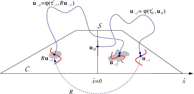
Figure 2. In proximity of a non-sticky state $\mathbf{u}_{0}$ that evolves backward in time into a state $\mathbf{u}_{-1}\notin\mathcal{S}$, a subset of $\mathcal{S}$ (the thick segment) is mapped into a subset of $\mathcal{C}$ of zero measure (the thick wiggly line). Furthermore, if $\mathbf{u}_{-1}$ evolves backward into $\mathbf{u}_{-2}\notin\mathcal{S}$ then $\mathcal{T}^{-}$ is a diffeomorphism between a neighborhood of $\mathbf{u}_{-1}$ and a neighborhood of $\mathbf{u}_{-2}$.

2.

Let us assume that a given pair $(\tau_{0}^{-},\mathbf{u}_{0})$ satisfies (89) with $\tau_{0}^{-}\neq 0$. If $\varphi(\tau_{0}^{-},\mathbf{u}_{0})\notin\mathcal{S}$, then

$$0\neq\left.\frac{\partial}{\partial\tau^{-}}\left(\varphi(\tau^{-},\mathbf{u})\cdot\mathbf{e}_{1}\right)\right|_{\tau_{0}^{-},\mathbf{u}_{0}}=\chi\left(\varphi(\tau_{0}^{-},\mathbf{u}_{0})\right)\cdot\mathbf{e}_{1}$$

and the implicit function theorem yields a smooth mapping $\tau^{-}$ in an open neighborhood of $(\tau_{0}^{-},\mathbf{u}_{0})$. However this map need not coincide with our inverse time of flight in the whole neighborhood, since it depends on the free flow $\varphi$ which does not take into account the presence of the floor. To overcome the problem, we argue as follows. If $\mathbf{u}_{0}\in\mathcal{S}$ we may not apply the transformation (90) to an entire open neighborhood of $\mathbf{u}_{0}$ in $\mathcal{C}$, because that neighborhood would necessarily contain points of $\mathcal{C}^{-}$, where (90) is not defined. Then, if $\mathbf{u}_{0}$ is a grazing, we consider a small open neighborhood $\mathcal{U}\subset\mathcal{S}$ of $\mathbf{u}_{0}$ in $\mathcal{S}$ containing only grazing states and satisfying $\mathcal{T}^{-}(\mathcal{U})\cap\mathcal{S}=\emptyset$. Since $R\mathbf{u}=\mathbf{u}$ if $\mathbf{u}\in\mathcal{S},$ we deduce that the restriction of $\mathcal{T}^{-}$ on $\mathcal{U}$ is as smooth as $\varphi$. If $\mathbf{u}_{0}$ is the beginning of a sticky event, then we can not consider an open neighborhood of $\mathbf{u}_{0}$ in $\mathcal{S}$ because it would contain states having $\tau^{-}=0$, and for those the transformation (90) is not defined. Then we consider open intervals $\tilde{\mathcal{U}}$ along the straight line defined by $\dot{x}=0$, $F=0$. If $\tilde{\mathcal{U}}$ is small enough, then it does not contain states for which $\dot{F}\geq 0$ and moreover $\mathcal{T}^{-}(\tilde{\mathcal{U}})\cap\mathcal{S}=\emptyset$. Then the restriction of $\mathcal{T}^{-}$ on $\tilde{\mathcal{U}}$ is as smooth as $\varphi$.

The union of all the above sets $\mathcal{U}$, $\tilde{\mathcal{U}}$ is

$$\bar{\mathcal{S}}=\left\{\mathbf{u}\in\mathcal{S}\left|\mathcal{T}^{-}(\mathbf{u})\,\mathrm{is\,defined\,and\,}\mathcal{T}^{-}(\mathbf{u})\notin\mathcal{S}\right.\right\}.$$

The set $\bar{\mathcal{S}}$ is contained in a two-dimensional plane and has zero measure in $\mathcal{C}^{+}$, which is three-dimensional, and the previous discussion proves that $\mathcal{T}^{-}$ is as smooth as $\varphi$ on $\bar{\mathcal{S}}$. Then the image of $\bar{\mathcal{S}}$ in $\mathcal{C}^{+}$ through $\mathcal{T}^{-}$, namely $\mathcal{T}^{-}(\bar{\mathcal{S}})$, is also a set of zero measure in $\mathcal{C}^{+}$, see e.g. [14, Chapter 2, Proposition 1.6]. By analogy, for $n\geq 2$, we define

$$\bar{\mathcal{S}}^{n}=\left\{\mathbf{u}\in\mathcal{T}^{-}(\bar{\mathcal{S}}^{n-1})\left|\mathcal{T}^{-}(\mathbf{u})\notin\mathcal{S}\right.\right\}$$

and we set $\bar{\mathcal{S}}^{1}=\bar{\mathcal{S}}$, $\bar{\mathcal{S}}^{0}=\mathcal{S}$. As before, $\mathcal{T}^{-}$ is smooth on $\bar{\mathcal{S}}^{n}$ and then, by induction, $\bar{\mathcal{S}}^{n+1}\subset\mathcal{T}^{-}(\bar{\mathcal{S}}^{n})$ has zero measure in $\mathcal{C}^{+}$ for every $n$. By the sigma-additivity of the Lebesgue measure, it follows that

$$\Sigma=\cup_{n=0}^{\infty}\bar{\mathcal{S}}^{n}$$

has zero measure, too.

The bouncing ball starting from an initial condition $\mathbf{u}\in\mathbb{R}^{4}$, with $\mathbf{u}\cdot\mathbf{e}_{1}>0$, will experience a grazing or a sticky event if its first contact state $\varphi(\tau(\mathbf{u}),\mathbf{u})$ satisfies

$$\varphi(\tau(\mathbf{u}),\mathbf{u})\in\Sigma.$$

So, the set $\mathcal{A}$ of anomalous initial conditions that reach $\mathcal{S}$ after a finite number of contacts is contained in

$$\cup_{t\leq 0}\varphi(t,\Sigma)=\varphi\left((-\infty,0]\times\Sigma\right)$$

which has zero measure in $\mathbb{R}^{4}$, by the smoothness of $\varphi$ with respect to all its variables.

We now prove that $\mathcal{A}$ is nowhere dense in $\mathbb{R}^{4}$. Because $\mathcal{A}$ has zero measure, no sphere centered in a point belonging to $\mathcal{A}$ is a subset of $\mathcal{A}$. Then we need to show that around each non-anomalous points there is a neighborhood that does not intersect $\mathcal{A}$.

Let us assume that $\mathbf{u}\notin\mathcal{A}$ . Let us call $\mathbf{u}(t)$ the state of the system at the time $t$, starting from the initial condition $\mathbf{u}$. From the results of section 3 it follows that after $N$ contacts it is $E(\mathbf{u}(t_{N}))<E_{min}$, where $E_{min}$ is the minimal energy required to have an anomalous contact (see Lemma (3.1)). Since the mechanical energy is a continous function of the state of the system, there is a neighborhood $\mathcal{V}$ of $\mathbf{u}(t_{N})$ such that $\mathcal{V}\cap\mathcal{S}=\emptyset$ and $E(\mathbf{v})<E_{min}$ if $\mathbf{v}\in\mathcal{V}$. Furthermore, $\mathcal{V}$ may be taken small enough to ensure that $\mathcal{T}^{-n}(\mathcal{V})\cap\mathcal{S}=\emptyset$ for $n=1,\cdots,N$. Finally, we observe that any neighborhood $\mathcal{U}$ of $\mathbf{u}$ such that $\varphi(\tau(\mathcal{U}),\mathcal{U})\subset\mathcal{T}^{-N}(\mathcal{V})$ does not intersect $\mathcal{A}$.

7. Numerical Results

7.1. On the Nature of the Restitution Coefficient

The dynamics of the mechanical system described in section (2) may be easily simulated on a digital computer, finding the instants of impact of the lower point mass with the floor with an accuracy as high as the machine precision.

If the mechanical system is left free to fall with its internal degree of freedom not excited (that is with initial conditions $\xi(0)=\dot{\xi}(0)=0$, $\psi(0)>0,$ and arbitrary $\dot{\psi}(0)$) the resulting dynamics may, initially, approximate that of the rigid ball model with constant restitution coefficient (eq. (1)), provided that the spring is weakly dissipative and sufficiently rigid, and that the energy of the initial condition is sufficiently high. An example is illustrated in figure

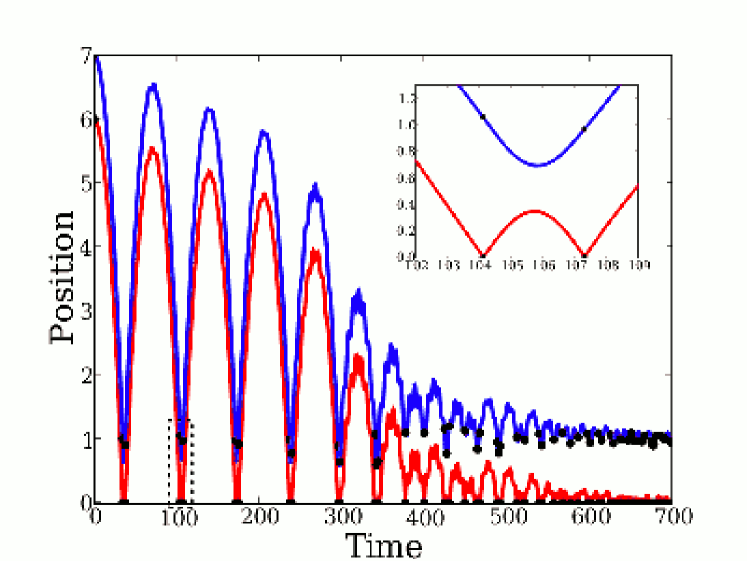
Figure 3. Numerical simulation with initial conditions $\xi(0)=\dot{\xi}(0)=\dot{\psi}(0)=0$, $\psi(0)=6$, and $\gamma=\mu=0.01$. The upper curve is $y(t)$, the lower curve is $x(t)$. The solid dots show the instants when there is an impact. The inset magnifies the region within the dashed rectangle.

(3), where the mechanical system is left free to fall from an height of six non-dimensional units.

This fact is explained by observing that, upon an impact, the vibrational and translational velocities exchange with each other (eq. (12)), so the center of mass of the ball has zero velocity just after the impact. In this situation we recognize three characteristic times

(91) $$T_{\psi}=\sqrt{\frac{1}{2\gamma}},\qquad T_{\xi}=\frac{\pi}{\sqrt{1-\mu^{2}}},\qquad T_{d}=\frac{1}{\mu}.$$

$T_{\psi}$ is the free-fall time of the center of mass, $T_{\xi}$ is half the proper period of the spring, and $T_{d}$ is the e-folding time associated with energy dissipation from the spring. If $T_{\psi}$ is much larger than $T_{\xi}$ then the center of mass does not have enough time to gain any appreciable speed before the expanding spring causes a second impact, which exchanges vibrational and translational velocities again. After this second impact the mechanical system is again propelled upward, with a very small vibrational energy left in the spring. At this point, if the kinetic energy of the center of mass is high enough to cause a time of flight to be of the order of $T_{d}$ or larger, then any residual vibrational energy will be dissipated to negligible levels during the flight, and the mechanical system will present itself to a third impact with the spring essential at rest, causing the double-impact dynamics described here to repeat itself.

In the limit $\gamma\rightarrow 0$ the residual vibrational energy tends to zero, and all dissipation happens during the double impact. Then it is appropriate to introduce the restitution coefficient

(92) $$r=\dot{\Psi}_{n}/\dot{\Psi}_{n+2}$$

where $\dot{\Psi}_{n}$ and $\dot{\Psi}_{n+2}$ are, respectively, the velocity of the center of mass before and after one of these double-impact events. It can be shown (see [15] for details) that it is

(93) $$r=e^{-\mu T_{\xi}}.$$

If we take our mechanical system as model of a bouncing ball, we are lead to say that during a double-impact event the ball is in contact with the floor: it takes this finite amount of time for the center of mass of the ball to exchange momentum with the floor and revert upward its velocity. Only flights longer than $T_{\xi}$ are to be taken as macroscopic flights. In the regime discussed here, our model may be seen as a version of the rigid ball model of eq. (1) in which the contacts have a finite, rather than infinitesimal, duration.

When, after a number of double-impact events, the time of flight becomes shorter than the characteristic dissipation time $T_{d}$, subsequent impacts will be able to store a significant amount of energy into the vibrational mode, subtracting it from the energy of the center of mass. This can be seen clearly in figure (3) where there is a sudden drop of the maximum height reached by the mechanical system between the fourth and the sixth macroscopic flight, and, at the same time, the trajectories of the two point masses become rather complicated and far from parabolic.

It is interesting a comparison between experiments in which a spherical bead is free to bounce repeatedly upon a rigid surface until it comes to rest, and our numerical simulations. Because the velocities of the center of mass of a bead are difficult to measure, it is customary in this kind of experiment to measure the time of flight, which is more accessible to the observer. In the experiments reported in [13] the coefficient of restitution is expressed as

(94) $$r_{n}=\frac{f_{n+1}}{f_{n}}$$

where $f_{n}$ is the time of flight of the bead, (which does not include the time of contact of the bead with the rigid surface). If the rigid ball model of eq. (1) is valid, then (94) is equivalent to the standard definition of restitution coefficient as ratio of velocities before and after the impact. If the bead is not rigid, then (94) must be taken as an alternate definition of restitution coefficient. In our numerical simulations, taking into account the interpretation of double-impacts as contact time with the floor, it is natural to define

(95) $$f_{n}=\tau_{2n}.$$

To simulate the very rigid tungsten carbide bead used in [13] we set $\gamma=10^{-5}$, while $\mu=0.01$ leads, according to the approximation (93), to the restitution coefficient $r=0.969\cdots$, which is about the same as what is measured in [13] for relatively high-velocity impacts. The simulated mechanical system, as the experimental bead, is left free-falling from a height equal to one quarter of its length. The restitution coefficient computed from the simulation, according to the definition (94), is shown in figure

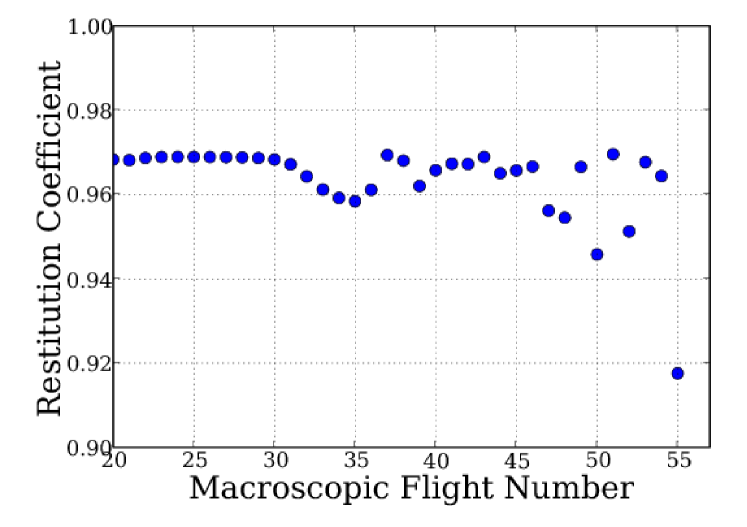
Figure 4. Restitution coefficient computed using the definition (94) from a simulation with $\gamma=10^{-5}$, $\mu=10^{-2}$, and initial conditions $\xi(0)=\dot{\xi}(0)=\dot{\psi}(0)=0,$ $\psi(0)=0.25$.

(4). Initially the value of $r$ is constant, and it is in excellent agreement with (93). Then $r$ declines, and finally it begins to fluctuate without a clear pattern. At even later times (not pictured in figure) the double-impact dynamics is completely disrupted, as in the case of figure (3), and the definition (95) ceases to be meaningful. This kind of behavior is qualitatively the same as that of the bead observed in [13] (see their figure (7)). In their case, after fluctuations in the value of $r$ of the same order of magnitude as those of figure (4), the bead is observed to vibrate while maintaining contact with the floor. We stress that the behavior of figure (4) remains qualitatively the same for any choice of parameters corresponding to slightly damped, very rigid springs.

A different way to look at the same dynamics is pictured in figure

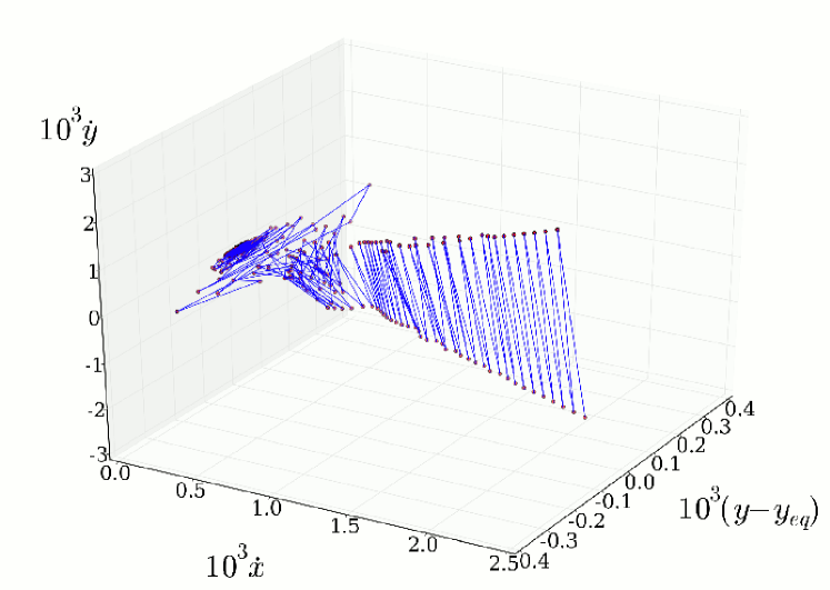
Figure 5. The dots represent the state of the system immediately after a contact with the floor (that is, $x=0$) for the simulation of figure (4). The equilibrium position of the upper point mass is $y_{eq}=1-2\gamma$. The thin lines have the sole purpose of making evident the temporal sequence of states.

(5) where we show the sequence of states belonging to the set $\mathcal{C}$ of contact configurations (87) for the same simulation that generated figure (4). Initially, the dynamics is clearly dominated by double-impacts, whose signature is the alternation of negative and positive values of $\dot{y}$, which gives a characteristic zig-zag look at the early part of the sequence. At later times the sequence of states becomes very disordered, and lacks any easily recognizable pattern, except a tendency to move towards the equilibrium point. Figure

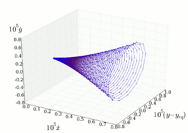
Figure 6. Magnification of the figure (5), close to $(0,0,0)$.

(6) is a magnification of figure (5) close to the equilibrium point. At these even later stages, the dynamics is well approximated by the map (85). The length of the spring and the velocity of the upper point mass are both subject to damped oscillations around the equilibrium position, and this gives a spiraling appearance to the sequence of states.

The reader may have noticed that the asymptotics of Theorem (2.1) are independent of the particular value of the damping parameter $\mu$. In particular, the results of the theorem apply equally to under-damped and over-damped oscillations. In figures

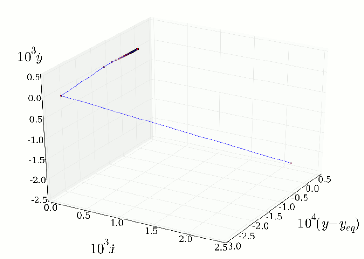
Figure 7. Same as figure (5), but with $\mu=2$.

(7) and

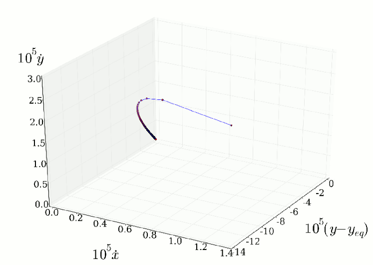
Figure 8. Magnification of figure (7), close to $(0,0,0)$.

(8) we show a simulation that uses $\gamma=10^{-5}$, $\mu=2$ and the same initial conditions as the simulation of figure (5). The length of the overdamped spring shrinks for the first few impacts, then slowly expands, approaching the equilibrium value monotonically from below. The system enters immediately the asymptotic regime, and the is no disordered transient. From a macroscopic point of view, the idealized ball may be taken as performing a single, totally inelastic impact with the floor.

7.2. Sticky Solutions

We have performed several numerical simulations using the following initial conditions

(96) $$\left\{\begin{array}[]{l}X_{0}=0\\ \dot{X}_{0}=\epsilon\\ Y_{0}=1+2\gamma-2\mu\dot{Y}_{0}\\ \dot{Y}_{0}=-0.1\end{array}\right..$$

For $\epsilon=0$ they obey the conditions (22), leading to a sticky event which lasts for $t_{c}=5.23\cdots$ non-dimensional time units. In figure

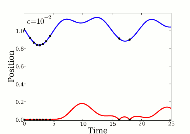
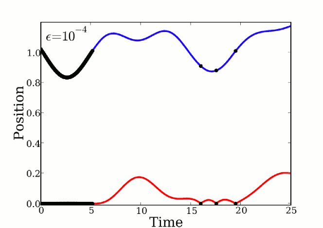
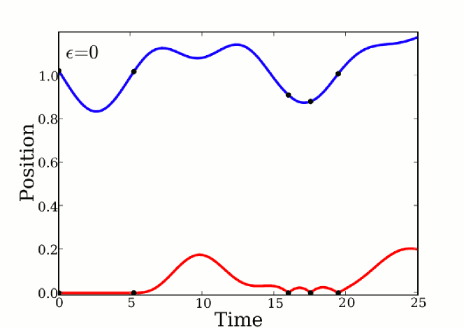
Figure 9. Simulations using the initial conditions (96) for three different values of $\epsilon$. Solid dots mark the times of impact. In the panel $\epsilon=0$, in the interval between the first two solid dots, the lower point mass is in contact with the floor.

(9) some sample trajectories are shown. It appears that, as $\epsilon$ decreases, the solutions tend to the solution with $\epsilon=0$. To quantify the convergence, we have computed the norm

(97) $$\left\|y_{\epsilon}-y_{s}\right\|=\sqrt{\frac{1}{t_{c}}\int_{0}^{t_{c}}(y_{\epsilon}(t)-y_{s}(t))^{2}dt}$$

where $y_{\epsilon}$ and $y_{s}$ are, respectively, the position of the upper point mass with $\epsilon\neq 0$, and with $\epsilon=0$. The results are shown in figure

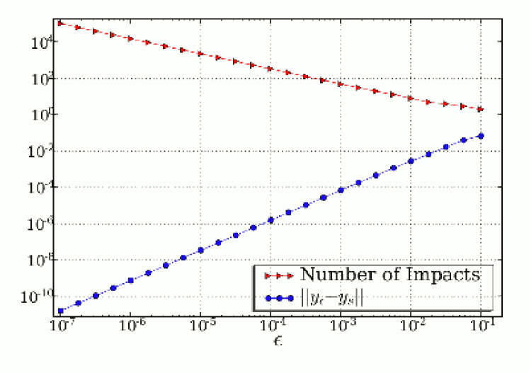
Figure 10. Number of impacts performed by the lower point mass in the interval $(0,t_{c})$ and root mean squared difference (97) as function of $\epsilon$.

(10). The root-mean-squared difference (97) falls to zero faster than linearly with $\epsilon$.

The numerical evidence supports the idea that the dynamics during a sticky event may be approximated up to any degree of accuracy by a non-sticky dynamics.

8. Discussion and Conclusions

Our simple model shows that taking into account explicitly the deformability of a bouncing body avoids the pathology of the inelastic collapse. Of course this comes at a price: our description of the bouncing ball, in spite of its simplicity, is considerably more complicated than a restitution-coefficient based model. This is affordable for one, or maybe a few, particles, but it is unbearable for systems with a very large number of bodies, even resorting to numerical simulation.

One may be tempted to overcome this difficulty by returning to a description based upon a restitution coefficient of the form

(98) $$r(u)=\left\{\begin{array}[]{lr}\exp\left(-\frac{\mu\pi}{\sqrt{1-\mu^{2}}}\right),&u>u_{c}\\ 1-\frac{\mu}{3\gamma}u,&u\leq u_{c}\end{array}\right.$$

where $u_{c}=3\gamma\mu^{-1}\left(1-\exp(-\mu\pi/\sqrt{1-\mu^{2}})\right)$. This is obtained by stitching the expression (93), which is valid for times of flight larger than the characteristic damping time of internal vibrations, and the coefficient in expression (86), which is the map that approximates the asymptotic vibrations of a ball close to equilibrium.

Although (98) is very accurate for large and for small values of $u$, a glance at the figures of section 7 shows that (for underdamped springs) there is an intermediate range of impact speeds where (98) simply fails. When the internal vibrational mode is excited, but the times of flight are not yet infinitesimal, the dynamics is too irregular to be parameterized with a velocity-dependent restitution coefficient.

We may hint that a satisfactory parameterization will need some form of bookkeeping of the energy stored in the internal vibrations, and some rule to determine the exchanges between that and the energy of the center of mass. At this stage, we are unable to suggest anything more specific than these vague considerations. In particular, it is not at all clear if accounting for internal vibrations will help the ongoing search for some sort of hydrodynamic limit for systems with a large number of dissipative particles.

We remark that the behavior of the bouncing ball, close to equilibrium, does not depend crucially on the linearity of the spring. A nonlinear variant of the model described in section (2) is embodied by the equations

(99) $$\left\{\begin{array}[]{c}\ddot{\psi}=-\gamma\\ \ddot{\xi}=-\rho\xi\left|\xi\right|^{a}-2\mu\dot{\xi}\left|\xi\right|^{b}\end{array}\right.$$

with $\rho,\mu>0$, $a,b\geq 0$. The impact times $t_{n}$ are determined by condition (11), where the collision rule (12) must be applied. The constraint $\psi(t)>\xi(t)$ holds at all times. We recover the linear model for $a=b=0$. It has been argued, on the basis of Hertz’s contact law, that the correct choice for modeling homogeneous spheres is $a=b=1/2$, and that the restitution coefficient (3) may be justified, for vanishing speeds of impact, by computing the energy dissipated by (99) in a single compression-expansion cycle (see [3] chap. 3 and references therein). Although some of the claims in the literature appear to be questionable in their generality, because the vector field defining (99) is non-Lipschitz for $\xi=0$ and $0<b<1$, the problem is well-posed close to the position of static equilibrium, which is

(100) $$\psi=\dot{\psi}=\dot{\xi}=0,\quad\xi=-\left(\frac{\gamma}{\rho}\right)^{\frac{1}{a+1}}.$$

That corresponds to the minimum of the energy

(101) $$E=\frac{\dot{\psi}^{2}}{2}+\frac{\dot{\xi}^{2}}{2}+\frac{\rho}{a+2}\left|\xi\right|^{a+2}+\gamma\psi$$

which is a non-increasing function of time:

$$\frac{dE}{dt}=-\mu\dot{\xi}^{2}\left|\xi\right|^{b}.$$

If we take a contact configuration $(0,\dot{X}_{0},Y_{0},\dot{Y}_{0})$ close enough to the static equilibrium (100) the system remains close to the minimum of the energy at all later times. As a consequence, we are guaranteed that $\ddot{X}_{n}$ and $\dddot{X}_{n}$ are in a neighborhood of $-2\gamma$ and $2\mu\gamma(\gamma/\rho)^{b/(a+1)}$, respectively. Then we follow the steps (48) through (51), using (57) as the time of flight, and we find that the asymptotic dynamics follows the map (85) with $\alpha_{n}\rightarrow\mu(3\gamma)^{-1}(\gamma/\rho)^{b/(a+1)}$ for $n\rightarrow\infty$. Then we conclude that a sequence of repeated impacts, because of the deformability of the body, follows the same asymptotic law as the linear case. As a consequence, the restitution coefficient (3) may be accurate only in the case of well-separated impacts, that is, when the time of flight between consecutive impacts is large enough to allow for dissipation of internal vibrations.

9. Appendix

Lemma 9.1.

Given the map

$$x_{n+1}=x_{n}-\alpha_{n}x_{n}^{2}+o(x_{n}^{2})$$

with $0<x_{0}\ll 1$ and $\lim_{n\rightarrow\infty}\alpha_{n}=\alpha>0$, then

$$\lim_{n\to\infty}x_{n}=0\quad and\quad\lim_{n\to\infty}nx_{n}=\frac{1}{\alpha}.$$

Proof.

Since $(\alpha_{n}-\alpha)x_{n}^{2}=o(x_{n}^{2})$, we may write

(102) $$x_{n+1}=x_{n}-\alpha x_{n}^{2}+o(x_{n}^{2}).$$

For small $x_{0}$, the sequence generated by (102) is positive, decreasing and $\lim_{n\to\infty}x_{n}=0$. For a given $\epsilon$, let us take $N$ such that for any $n>N$

(103) $$1-(a+\epsilon)x_{n}\leq\frac{x_{n+1}}{x_{n}}\leq 1-(a-\epsilon)x_{n}$$

We may assume $x_{N}<1/(\alpha-\epsilon)$ , then $x_{N+k}<1/(\alpha-\epsilon)$; we prove that $x_{N+k}\leq 1/k(\alpha-\epsilon)$ implies $x_{N+k+1}\leq 1/(k+1)(\alpha-\epsilon)$ and apply induction. Multiplying the right inequality in (103) by $1+(a-\epsilon)x_{n}$, we have

$$\frac{x_{n+1}}{x_{n}}(1+(a-\epsilon)x_{n})\leq 1$$

Then

$$x_{N+k+1}\leq\frac{x_{N+k}}{1+(a-\epsilon)x_{N+k}}$$

where $x/1+(a-\epsilon)x$ is an increasing function of $x$ and $x_{N+k}\leq 1/k(\alpha-\epsilon)$, then

$$x_{N+k+1}\leq\frac{\frac{1}{k(\alpha-\epsilon)}}{1+(a-\epsilon)\frac{1}{k(\alpha-\epsilon)}}=\frac{1}{(k+1)(\alpha-\epsilon)}.$$

By induction

$$x_{n}\leq\frac{1}{(n-N)(\alpha-\epsilon)}\quad\forall n>N$$

then

$$\limsup_{n\rightarrow\infty}nx_{n}\leq\frac{1}{\alpha-\epsilon}\qquad\forall\varepsilon>0$$

i.e.

$$\limsup_{n\to\infty}nx_{n}\leq\frac{1}{\alpha}.$$

By a similar argument we get

$$\liminf_{n\to\infty}nx_{n}\geq\frac{1}{\alpha}$$

which proves the proposition. ∎

Remark 9.2.

It follows that for a map $x_{n+1}=x_{n}-\alpha x_{n}^{\beta}+o(x_{n}^{\beta})$ , with $\beta>1$,

(104) $$\lim_{n\to\infty}x_{n}=0\quad{\mathrm{and}}\quad\lim_{n\to\infty}n^{\frac{1}{\beta-1}}x_{n}>0.$$

This can be seen by using the transformation $z_{n}=x_{n}^{\beta-1}$. We have

$$\frac{z_{n+1}}{z_{n}}=\left(1-\alpha x_{n}^{\beta-1}+o(x_{n}^{\beta-1})\right)^{\beta-1}=1-\alpha(\beta-1)x_{n}^{\beta-1}+o(x_{n}^{\beta-1})$$

We then apply Lemma 9.1 to

$$z_{n+1}=z_{n}-\alpha(\beta-1)z_{n}^{2}+o(z_{n}^{2})$$

which gives (104).

Lemma 9.3.

If $x_{n}>0$ and $x_{n+1}=x_{n}+O(x_{n}^{2})$ then $\sum_{n}x_{n}=+\infty$.

Proof.

We have $x_{n+1}\geq x_{n}-cx_{n}^{2}$ for a suitable $c>0$. Hence, if we define

$$\left\{\begin{array}[]{ccc}z_{n+1}&=&z_{n}-cz_{n}^{2}\\ z_{0}&=&x_{0}\end{array}\right.$$

we have $x_{n}\geq z_{n}$ for all $n\geq 0$. Applying Lemma (9.1) to this map, the thesis follows. ∎

Lemma 9.4.

If there exists a sequence $\left\{\alpha_{n}\right\}_{n\in\mathbb{N}}$ with $\alpha_{n}\in(0,1)$ that satisfies (67), then $\lim_{n\rightarrow\infty}\alpha_{n}=0$.

Proof.

Let us define the functions $f$ and $g$ as

(105) $$f(x)=6x-4x^{2}+x^{3},$$

(106) $$g(x)=\frac{6x-8x^{2}+3x^{3}}{\left(1-x\right)^{3}}.$$

The map (67) is then written as

(107) $$f(\alpha_{n+1})=g(\alpha_{n})+b_{n},$$

with $b_{n}\to 0$. Since $f$ is bounded in $[0,1]$ and $g$ tends to $\infty$ as $x\to 1$, it is easy to see that there exists $\delta>0$ such that $\alpha_{n}\leq 1-\delta$. We observe, that $f^{\prime}(x)>0$. With some algebra, we also find, for $x\in[0,1)$,

(108) $$f(x)-g(x)\leq-\frac{x^{2}}{(1-x)^{3}}.$$

In particular, the map (67) has no fixed point in $(0,1)$. Let us assume that $\{\alpha_{n}\}$ does not converge to zero. This means $\alpha_{n}\geq\epsilon$ for infinitely many values of $n$ and some $\epsilon>0$. Inequality (108) implies that $g(x)-f(x)\leq-\epsilon^{2}$ for $x\geq\epsilon$. Let us fix $m$ such that $|b_{n}|\leq\epsilon^{2}/2$ for $n\geq m$ and take any $\alpha_{n}\geq\epsilon$ with $n\geq m$. Then the inequality $\alpha_{n+1}\leq\alpha_{n}$ would give, since $f$ is increasing,

$$b_{n}=f(\alpha_{n+1})-g(\alpha_{n})\leq f(\alpha_{n})-g(\alpha_{n})\leq-\epsilon^{2}$$

which contradicts the choice of $b_{n}$. Therefore $\alpha_{n+1}>\alpha_{n}\geq\epsilon$ and, iterating this argument, the sequence $\alpha$ is eventually increasing and convergent to a number $0<\alpha<1$ satisfying $f(\alpha)=g(\alpha)$. Since this contradicts (108), the proof is complete. ∎

References

- [1] R. Cross, The Coefficient of Restitution for Collisions of Happy Balls, Unhappy Balls, and Tennis Balls, Am. J. Phys., 68, 1025-1031 (2000).
- [2] J. Guckenheimer, P. Holmes, Nonlinear Oscillations, Dynamical Systems and Bifurcations of Vector Fields, Springer, Berlin/Heidelberg (1983).
- [3] N. V. Brilliantov, T. Pöschel, Kinetic Theory of Granular Gases, Oxford University Press, Oxford, (2004).
- [4] S. McNamara and W. R. Young, Inelastic Collapse and Clumping in a One-Dimensional Granular Medium, Phys. Fluids A, 4, 496-504, (1992).
- [5] N. Schörghofer and T. Zhou, Inelastic Collapse of Rotating Spheres, Phys. Rev. E, 54, 5511-5515, (1996).
- [6] R. Ramírez, T. Pöschel, N. V. Brilliantov, and T. Schwager, Coefficient of restitution of colliding viscoelastic spheres, Phys. Rev. E, 60, 4465-4472, (1999).
- [7] F. G. Bridges, A. Hatzes, and D. N. Lin, Structure, Stability and Evolution of Saturn’s Rings, Nature, 309, 333-335, (1984).
- [8] D. Goldman, M. D. Shattuck, C. Bizon, W. D. McCormick, J. B. Swift, and H. L. Swinney, Absence of Inelastic Collapse in a Realistic Three Ball Model, Phys. Rev. E, 57, 4831-4833, (1998).
- [9] J. Duran, Sands, Powders, and Grains: An Introduction to the Physics of Granular Materials, Springer, Berlin/Heidelberg (1999).
- [10] S. Luding, S. McNamara, How to Handle the Inelastic Collapse of a Dissipative Hard-Sphere Gas with the TC Model, Granular Matter, 1, 113-128, (1998).
- [11] T. Aspelmeier, A. Zippelius, Dynamics of a One-Dimensional Granular Gas with a Stochastic Coefficient of Restitution, Physica A, 282, 450-474, (2000).
- [12] M. di Bernardo, C. Budd, A. Champneys, P. Kowalczyk, Piecewise-smooth Dynamical Systems: Theory and Applications, Springer, Berlin/Heidelberg, 2007.
- [13] E. Falcon et al., Behavior of one inelastic ball bouncing repeatedly off the ground; Eur. Phys. J. B, 3, 45-57, (1998).
- [14] M. Golubitsky, V. Guillemin, Stable Mappings and Their Singularities, Springer, Berlin/Heidelberg, 1973.
- [15] F. Paparella and G. Passoni, Absence of inelastic collapse for a one-dimensional gas of grains with an internal degree of freedom; Comp. Math. App. (2007), in press.