Towards a microscopic theory of toroidal moments in bulk periodic crystals

Abstract

We present a theoretical analysis of magnetic toroidal moments in periodic systems, in the limit in which the toroidal moments are caused by a time and space reversal symmetry breaking arrangement of localized magnetic dipole moments. We summarize the basic definitions for finite systems and address the question of how to generalize these definitions to the bulk periodic case. We define the toroidization as the toroidal moment per unit cell volume, and we show that periodic boundary conditions lead to a multivaluedness of the toroidization, which suggests that only differences in toroidization are meaningful observable quantities. Our analysis bears strong analogy to the “modern theory of electric polarization” in bulk periodic systems, but we also point out some important differences between the two cases. We then discuss the instructive example of a one-dimensional chain of magnetic moments, and we show how to properly calculate changes of the toroidization for this system. Finally, we evaluate and discuss the toroidization (in the local dipole limit) of four important example materials: BaNiF₄, LiCoPO₄, GaFeO₃, and BiFeO₃.

I Introduction

The recent resurgence of interest in magneto-electric multiferroics has prompted discussion of the relevance of the concept of magnetic toroidal moments in such systems (see e.g. Refs. Schmid, 2001, 2003, 2004; Fiebig, 2005; Arima et al., 2005; Sawada and Nagaosa, 2005; Van Aken et al., 2007). A magnetic toroidal moment is represented by a time-odd polar (or “axio-polar”, see Ref. Ascher, 1974) vector, which changes sign under both time inversion and space inversion, and is generally associated with a “circular” or “ring-like” arrangement of spins (see Fig. 1 for some examples).Dubovik and Tugushev (1990) Materials in which the toroidal moments are aligned cooperatively – so-called ferrotoroidics – have been proposed to complete the group of primary ferroics.Schmid (2003, 2004); Van Aken et al. (2007) Further interest stems from the fact that the toroidal moment is related to the antisymmetric part of the linear magneto-electric tensor;Gorbatsevich et al. (1983); Sannikov (1997) this points to an important role played by the magnetic toroidal moment for magneto-electric coupling phenomena.

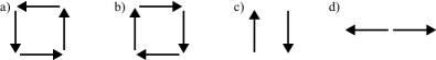
Figure 1: Simple arrangements of magnetic moments which can lead to toroidal moments. (a) and (b) have equal and opposite toroidal moments. The antiferromagnetic arrangement in (c) has a toroidal moment, whereas that in (d) does not.

Magnetic toroidal moments in condensed matter systems were first studied in the former Soviet Union during the 1980s, mostly in the context of the so-called “excitonic insulator” model (see Refs. Dubovik and Tugushev, 1990; Gorbatsevich and Kopaev, 1994 for reviews of this work). At about the same time, Sannikov and Zheludov proposed the toroidal moment as the primary order parameter for the low temperature phase transition in multiferroic nickel iodine boracite.Sannikov and Zheludov (1985) Since in these early studies the toroidal moment was mostly treated as a macroscopic order parameter, no particular attention was paid to the peculiarities arising from the microscopic definition of the toroidal moment. It is therefore the purpose of the present paper to give a detailed analysis of the properties of toroidal moments starting from the microscopic definition and focusing especially on effects resulting from the periodic boundary condition in crystalline solids. In particular, we address the following questions:

1. How should the toroidal moment density, or toroidization, of a bulk periodic solid be formally defined?

2. Is there a consistent way to treat the origin dependence of the toroidal moment?

3. What are the consequences of the periodic boundary conditions within a bulk crystalline solid?

In addition, we apply our newly developed concepts to evaluate and analyze the toroidization of four example materials: the antiferromagnetic ferroelectrics BaNiF₄ and BiFeO₃, the polar ferrimagnet GaFeO₃, and the strongly magneto-electric material LiCoPO₄.

To avoid confusion, we point out that there also has been some recent discussion about electric toroidal moments $\bm{g}$, defined as $\bm{g}=\frac{1}{2}\sum_{i}\bm{r}_{i}\times\bm{p}_{i}$ where $\bm{p}_{i}$ is the local electric dipole moment at position $\bm{r}_{i}$ and the summation extends over all dipole moments in the system.Dubovik and Tugushev (1990); Naumov et al. (2004); Prosandeev et al. (2006) The vector $\bm{g}$ is fundamentally different from the magnetic toroidal moment, since it is both time- and space-inversion symmetric. It has been used to characterize circular domains in nano-scale ferroelectric materials.Naumov et al. (2004); Prosandeev et al. (2006) In the following we exclusively discuss the case of magnetic toroidal moments, i.e. the term “toroidal moment” is always used in the sense of “magnetic toroidal moment”. We point out, however, that some of our general considerations regarding origin-dependence and the effect of periodic boundary conditions are applicable to the case of electric toroidal moments as well.

This paper is organized as follows. We begin by summarizing some of the basic definitions and then discuss the limit where the toroidal moment is caused by a time and space reversal symmetry breaking arrangement of localized magnetic moments (Sec. II). In Sec. III we then analyze the origin dependence of the toroidal moment by decomposing the magnetic moment distribution into a fully compensated, generally non-collinear, antiferromagnetic part and a non-compensated, collinear, ferromagnetic part. In Sec. IV we define the toroidization as the toroidal moment per unit cell volume, and we show that the periodic boundary conditions lead to a multivaluedness of the toroidization, similar to the case of the electric polarization in bulk periodic solids (see Refs. King-Smith and Vanderbilt, 1993; Vanderbilt and King-Smith, 1993; Resta, 1994). This multivaluedness suggests that, as in the case of the electric polarization, only differences in toroidization can be physically observable quantities. In Sec. V we illustrate some consequences of the periodicity by using the example of a one-dimensional antiferromagnetic chain of magnetic moments. In Sec. VI we evaluate the toroidizations of four example materials: BaNiF₄, LiCoPO₄, GaFeO₃, and BiFeO₃. Finally, in Sec. VII we summarize our main conclusions and discuss the correspondence between the microscopic toroidal moment described in this paper and some phenomenological quantities with the same symmetry, that have recently appeared in the multiferroics literature.

II Definitions

The toroidal moment $\bm{t}$ corresponding to a current density distribution $\bm{j}(\bm{r})$ is defined as (see Ref. Dubovik and Tugushev, 1990):

$$\bm{t}=\frac{1}{10c}\int\left(\bm{r}(\bm{r}\cdot\bm{j})-2r^{2}\bm{j}\right)d^{3}r\quad,$$ (1)

where $c$ indicates the speed of light in vacuum. The toroidal moment in the form of Eq. (1) emerges from the multipole expansion of an arbitrary localized current distribution.Dubovik and Tugushev (1990) Its physical significance can be seen by noting that Eq. (1) is identically satisfied by the current distribution

$$\bm{j}(\bm{r})=c\nabla\times\nabla\times\delta(\bm{r})\bm{t}\quad,$$ (2)

which represents an elemental toroidal moment centered at the origin. Evaluating the interaction energy $E$ of this current density with the electromagnetic field $\bm{A}(\bm{r})$ yields (after partial integration):

$$E=-\frac{1}{c}\int\bm{j}(\bm{r})\cdot\bm{A}(\bm{r})\,d^{3}r=-\bm{t}\cdot\nabla\times\bm{B}(0)\quad,$$ (3)

where $\bm{B}(0)=\nabla\times\bm{A}(\bm{r})|_{\bm{r}=0}$ is the magnetic field at the site of the toroidal moment. From Eq. (3) it can be seen that the toroidal moment couples to the curl of the magnetic field such that a toroidal system in a magnetic field has lowest energy when its toroidal moment is aligned parallel to the curl of the magnetic field.

The definition of the toroidal moment can be re-cast into a more convenient form, by noting that the current vector can be decomposed into longitudinal ($\nabla\times\bm{j}_{\parallel}=0$) and transversal ($\nabla\cdot\bm{j}_{\perp}=0$) parts. The longitudinal part of $\bm{j}(\bm{r})$ is related to time derivatives of the charge multipole moments through the continuity equation $\dot{\rho}+\nabla\cdot\bm{j}=0$, and does not contribute to the toroidal moment.Dubovik and Tugushev (1990) The transverse part of the current density $\bm{j}_{\perp}(\bm{r})$ can be written as the curl of the magnetization density $\bm{\mu}(\bm{r})$:foo (a)

$$\bm{j}_{\perp}(\bm{r})=c\nabla\times\bm{\mu}(\bm{r})\quad.$$ (4)

Inserting Eq. (4) in Eq. (1) gives the toroidal moment in terms of $\bm{\mu}(\bm{r})$:foo (b)

$$\bm{t}=\frac{1}{2}\int\bm{r}\times\bm{\mu}(\bm{r})\,d^{3}r\quad.$$ (5)

While in principle, for a finite system with known magnetization density, this expression can be used to evaluate the toroidal moment, it is not directly applicable to extended systems where periodic boundary conditions are employed. The difficulties resemble those encountered in early attempts to calculate the electric polarization (see Ref. Resta, 1994): for a general continuous magnetization density $\bm{\mu}(\bm{r})$, Eq. (5) evaluated over one unit cell will lead to arbitrary values, depending on the special choice of unit cell used in the calculation.

In the case of the electric polarization, a general solution to this problem is achieved by evaluating the electric polarization directly from the electronic wave-function using Wannier representations.King-Smith and Vanderbilt (1993); Vanderbilt and King-Smith (1993); Resta (1994) In principle, a similar approach seems appropriate for the case of the toroidal moment. In the present paper, we pursue a somewhat simpler yet rather instructive approach by assuming that the magnetization density can be well represented by a distribution of localized magnetic moments $\{\bm{m}_{\alpha}\}$ at sites $\bm{r}_{\alpha}$:

$$\bm{\mu}_{\text{loc}}(\bm{r})=\sum_{\alpha}\bm{m}_{\alpha}\delta(\bm{r}-\bm{r}_{\alpha})\quad.$$ (6)

This results in the toroidal moment:

$$\bm{t}=\frac{1}{2}\sum_{\alpha}\bm{r}_{\alpha}\times\bm{m}_{\alpha}\quad.$$ (7)

The simplification to localized magnetic moments avoids the technical difficulties of a full gauge invariant wave-function formulation but retains all the peculiarities resulting from the periodic boundary conditions within bulk systems. It also allows a more intuitive analysis of several important prototype systems. Our study thus represents a first step towards a full microscopic theory of toroidal moments in crystalline solids and can be used as the basis for future developments.

We note however, that in some cases the restriction to localized magnetic moments can represent a severe simplification. Obviously, the local moment picture neglects the possibility of toroidal moments arising from non-localized magnetization densities, but in addition the symmetry of the magnetic moment distribution in Eq. (6) can eventually be higher than the full magnetic space group symmetry represented by the original magnetization density $\bm{\mu}(\bm{r})$. This can occur even in systems that are usually well described in terms of localized magnetic moments (see for example our discussion of BiFeO₃ in Sec. VI.4). The localized moment approach also neglects the possibility that the localized current distribution around the atomic site, which gives rise to the local magnetic dipole moment, simultaneously gives rise to a localized toroidal dipole moment. Such “atomic” toroidal moments have been discussed in the context of atomic multipole moments and can in principle be measured by resonant x-ray spectroscopy.Di Matteo et al. (2005) Here, we restrict our discussion to the case of toroidal moments “on the unit cell scale” and disregard the possibility of toroidal contributions “on the atomic scale”.

Using Eq. (7) we can straightforwardly evaluate the toroidal moments of the arrangements shown in Fig. 1. Taking the horizontal magnetic moments to be spaced a distance $a$ apart along the $y$ direction, and the vertical moments a distance $a$ apart along $x$, the toroidal moments of arrangements a) and b) in Fig. 1 are $\bm{t}=\pm as\hat{\bm{z}}$, where $s$ is the magnitude of the individual magnetic moments. The toroidal moment of Fig. 1c is $\bm{t}=-\frac{1}{2}as\hat{\bm{z}}$, whereas it is zero for the arrangement shown in Fig. 1d, since in this case the moment vectors are aligned parallel to the vector connecting the two sites.

III Origin dependence

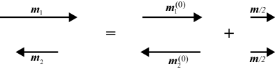
Figure 2: Decomposition of a ferrimagnetic arrangement of two localized moments (left) into its fully compensated component (middle) and its uncompensated “ferromagnetic” component (right). The ferromagnetic component at each site is the total magnetic moment divided by the total number of moments, $\tilde{\bm{m}}_{\alpha}=\frac{1}{2}(\bm{m}_{1}+\bm{m}_{2})$, and the compensated part is the difference between the magnitude of the original local moment and the uncompensated contribution.

It can easily be seen that for systems with non-vanishing magnetic dipole moment,

$$\bm{m}=\frac{1}{2c}\int\bm{r}\times\bm{j}(\bm{r})d^{3}r=\int\bm{\mu}(\bm{r})d^{3}r=\sum_{\alpha}\bm{m}_{\alpha}\quad,$$ (8)

the toroidal moment in Eqs. (1), (5), and (7) depends on the choice of origin. In particular, for a change of origin defined by $\bm{r}\rightarrow\bm{r}^{\prime}=\bm{r}+\bm{R}_{0}$ the toroidal moment changes as $\bm{t}\rightarrow\bm{t}^{\prime}=\bm{t}+1/2\bm{R}_{0}\times\bm{m}$.

To further analyze this origin dependence, we decompose the original magnetic moment distribution $\{\bm{m}_{\alpha}\}$ into two parts: a totally compensated part $\{\bm{m}_{\alpha}^{(0)}=\bm{m}_{\alpha}-\bm{m}/N\}$, with no net magnetization, $\sum_{\alpha}\bm{m}_{\alpha}^{(0)}=0$, and an uncompensated “ferromagnetic” part $\{\tilde{\bm{m}}_{\alpha}=\bm{m}/N\}$, where $\bm{m}=\sum_{\alpha}\bm{m}_{\alpha}$ is the total magnetic moment and $N$ is the total number of localized moments (see Fig. 2 for a simple example). This results in a corresponding decomposition of the toroidal moment into:

$$\bm{t}^{(0)}=\frac{1}{2}\sum_{\alpha}\bm{r}_{\alpha}\times\bm{m}_{\alpha}^{(0)}\quad,$$ (9)

and

$$\tilde{\bm{t}}=\frac{1}{2}\,\bar{\bm{R}}\times\bm{m}\quad,$$ (10)

where $\bar{\bm{R}}=1/N\sum_{\alpha}\bm{r}_{\alpha}$ is the average magnetic moment position. By construction, only the toroidal moment $\tilde{\bm{t}}$ depends on the choice of origin, whereas the part $\bm{t}^{(0)}$ is origin independent.

For a macroscopic toroidal moment to occur, the magnetic moment distribution has to break both time and space reversal symmetries. In the compensated moment distribution $\{\bm{m}^{(0)}_{\alpha}\}$ this can happen in several ways, depending both on how the magnetic moments are oriented and on how they are positioned. On the other hand the uncompensated distribution $\{\tilde{\bm{m}}_{\alpha}\}$ provides less freedom. Due to the non-vanishing magnetic dipole moment, the configuration $\{\tilde{\bm{m}}_{\alpha}\}$ always breaks time reversal symmetry. However, the only possibility for such a “ferromagnetic” moment distribution to simultaneously break space inversion symmetry is that the magnetic moments are positioned in a non-centrosymmetric way. A nonzero toroidal moment of the uncompensated part of any moment distribution is therefore always related to an inversion symmetry-breaking arrangement of the underlying ionic lattice, whereas this does not necessarily have to be the case for the compensated moment distribution $\{\bm{m}_{\alpha}^{(0)}\}$, where the inversion symmetry can also be lifted by the orientation of the various magnetic moments.foo (c)

It will become clear in the following section, that only differences in toroidal moment should have any physical significance. In the case of the origin-dependent part $\tilde{\bm{t}}$, such differences in toroidal moment must be related to corresponding displacements of the moment positions, and the change in the toroidal moment is then given by $\Delta\tilde{\bm{t}}=1/2\Delta\bar{\bm{R}}\times\bm{m}$, with $\Delta\bar{\bm{R}}=1/N\sum_{\alpha}\Delta\bm{r}_{\alpha}$ and $\Delta\bm{r}_{\alpha}$ being the displacements of the individual magnetic moments. Thus, if a consistent choice of origin is used for the initial and final configuration, the corresponding change in the toroidal moment is a well-defined physical quantity. For example, if the initial reference configuration is centrosymmetric, then the change in toroidal moment resulting from a symmetry-breaking structural distortion can be interpreted as the spontaneous toroidal moment of the system.

Earlier applications of Eq. (7) did not perform the explicit decomposition described above, but instead evaluated the toroidal moment with respect to the “center of the unit cell”,Popov et al. (1998) without specifying exactly how this center of the unit cell is defined. We point out that the origin dependent contribution to the toroidal moment $\tilde{\bm{t}}$ vanishes, if the “center of the unit cell” defined by $\bar{\bm{R}}$ is taken as the origin.foo (d) However, it is important to realize that for cases where the toroidal moment changes as a result of a structural distortion, $\bar{\bm{R}}$ in general also changes (see the discussion in the previous paragraph). In such cases the origin should be taken to be the same for both structural modifications.

Finally, we note that in the case of a non-localized magnetization density, the “uncompensated” part of $\bm{\mu}(\bm{r})$ would correspond to a uniform, i.e. perfectly homogeneous ($\bm{r}$-independent), magnetization density $\tilde{\bm{\mu}}=\bm{m}/V$, where $V$ is the total volume of the system. Since such a perfectly homogeneous magnetization density $\tilde{\bm{\mu}}$ can never break space-reversal symmetry, it does not contribute at all to the toroidal moment of the system. Thus, in a non-localized description, the decomposition into compensated and uncompensated parts results in a perfect separation between dipolar and toroidal contributions to the magnetization density. Due to the “inhomogeneity” that is intrinsic to the localized moment description, the decomposition is not fully complete in this case, and the toroidal contribution of the “ferromagnetic” part has to be analyzed separately.

In our explicit examples in Secs. V and VI we will only consider systems with fully compensated moment configurations and postpone the further analysis of toroidal moments resulting from “ferromagnetic” configurations to future work.

IV The case of a periodic bulk system

We now proceed to the case of bulk periodic crystals with an infinite periodic arrangement of magnetic moments. We begin by defining the toroidal moment per unit volume or toroidization $\bm{T}=\bm{t}/V$, where $V$ is the volume of the system with toroidal moment $\bm{t}$. Then, for a large finite system containing $N$ identical unit cells each of volume $\Omega$:

$$\bm{T} =\frac{1}{2N\Omega}\sum_{\alpha}\bm{r}_{\alpha}\times\bm{m}_{\alpha}$$ (11)

$$=\frac{1}{2N\Omega}\sum_{n,i}(\bm{r}_{i}+\bm{R}_{n})\times\bm{m}_{i}\quad.$$ (12)

Here, $\bm{r}_{i}$ are the positions of the magnetic moments $\bm{m}_{i}$ relative to the same (arbitrary) point within each unit cell, $\bm{R}_{n}$ is a “lattice vector” with index $n$, and we have used the fact that the orientation of the magnetic moments is the same in each unit cell. The summation over $i$ indicates the summation over all moments within a unit cell, and that over $n$ indicates the summation over all unit cells. Expanding the cross product, we obtain:

$$\bm{T} =\frac{1}{2\Omega}\sum_{i}\bm{r}_{i}\times\bm{m}_{i}+\frac{1}{2N\Omega}\sum_{n}\bm{R}_{n}\times\sum_{i}\bm{m}_{i}$$ (13)

$$=\frac{1}{2\Omega}\sum_{i}\bm{r}_{i}\times\bm{m}_{i}+\frac{1}{2N^{2}\Omega}\sum_{n}\bm{R}_{n}\times\bm{m}$$ (14)

$$=\frac{1}{2\Omega}\sum_{i}\bm{r}_{i}\times\bm{m}_{i}\quad,$$ (15)

where in the last step we have assumed that the sum over all lattice vectors contains both $\bm{R}_{n}$ and $-\bm{R}_{n}$, so that $\sum_{n}\bm{R}_{n}=0$. This is true for any infinite Bravais lattice. Thus, the toroidal moment of a system of $N$ unit cells is just $N$ times the toroidal moment evaluated for one unit cell, and the corresponding toroidizations are identical.

In an infinite periodic solid, we have a freedom in choosing the basis corresponding to the primitive unit cell of the crystal. In particular, we can translate any spin of the basis by a lattice vector $\bm{R}_{n}$ without changing the overall periodic arrangement. However, such a translation of magnetic moment $\bm{m}_{i}$ by $\bm{R}_{n}$ leads to a change in the toroidization as follows:

$$\Delta\bm{T}_{ni}=\frac{1}{2\Omega}\bm{R}_{n}\times\bm{m}_{i}\quad.$$ (16)

The freedom in choosing the basis corresponding to the primitive unit cell thus leads to a multivaluedness of the toroidization with respect to certain “increments” (defined by Eq. (16)) for each magnetic sub-lattice $i$ and lattice vector $\bm{R}_{n}$.

This multivaluedness of the toroidization is in strong analogy to the modern theory of electric polarization,King-Smith and Vanderbilt (1993); Vanderbilt and King-Smith (1993); Resta (1994) where the polarization changes by $e\bm{R}_{n}/\Omega$ if one translates an elementary charge $e$ by a multiple of a lattice vector $\bm{R}_{n}$. The resulting multivaluedness has led to the concept of the “polarization lattice” corresponding to a bulk periodic solid,Vanderbilt and King-Smith (1993) with $e\bm{R}_{n}/\Omega$ called the “polarization quantum” if $\bm{R}_{n}$ is one of the three primitive lattice vectors. Eq. (16) suggests the existence of an analogous “toroidization lattice”. However, the vector product in Eq. (16) and our classical treatment of magnetic moments can lead to arbitrary projections of $\bm{m}_{i}$ on a certain axis, and therefore the structure of the “toroidization lattice” is quite different from that of the polarization lattice. In the most general case, if there are $r$ magnetic basis atoms in the primitive unit cell, there can be 3$r$ linearly independent toroidization increments. This can lead to cases, where multiple incommensurate increments exist along certain crystallographic directions. In addition, for a collinear moment configuration no toroidization component is allowed parallel to the global magnetic axis. Thus, the set of allowed toroidization values does not necessarily have the same translation symmetry as the corresponding crystal structure and does not necessarily form a Bravais lattice, whereas this is always true in the case of the electric polarization. In practice, the magnetic symmetry of the system can significantly reduce the number of linearly independent toroidization increments (see Sec. VI for some realistic examples.

In spite of the difficulties associated with the multivaluedness of the polarization, it is now recognized that only differences in the polarization lattices between different ionic configurations are in fact measurable quantities, such as for example the difference between two oppositely polarized states of a ferroelectric crystal or between a centrosymmetric non-polar reference structure and the actual polar crystal. These differences are the same for each point of the polarization lattice and are thus well-defined quantities. In analogy with the case of the electric polarization we suggest that only differences in the set of allowed toroidization values, corresponding to two different bulk configurations, are physically observable quantities, such as the difference in toroidizations between two domain states of a ferrotoroidic, or the difference between a ferrotoroidic state and its non-toroidic paraphase. Such quantities can be obtained by monitoring the change in toroidal moment on one arbitrarily chosen branch within the allowed set of values, when transforming the system from the initial to the final state along a well-defined path.

Finally, we emphasize that the multivaluedness of the toroidization and the possible origin dependence of the toroidization are two independent features with different origins. Both features are rooted in the fundamental definition of the toroidal moment in terms of the position operator $\bm{r}$, but whereas the origin dependence appears in both finite and infinite systems if there is a non-vanishing magnetic dipole moment, the multivaluedness is caused by the periodic boundary conditions in a bulk solid, and is independent of an eventually non-vanishing magnetic dipole moment.

V A one-dimensional example

V.1 The periodic non-toroidal state

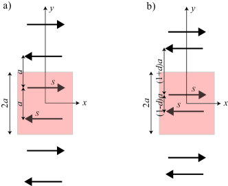
Figure 3: Calculation of the toroidization for two different one-dimensional antiferromagnetic periodic arrangements of magnetic moments. Our choice of unit cell is indicated by the shaded area in each case. a) shows a non-toroidal state, which is space-inversion symmetric with respect to each moment site. b) is a toroidal state.

To illustrate some consequences of the multivaluedness of the toroidization in periodic systems described in the previous section, we now consider the example of a one-dimensional antiferromagnetic chain of equally spaced magnetic moments as shown in Fig. 3a. The moments, with magnitude $s$, are spaced a distance $a$ apart from each other along the $y$ axis, and are alternating in orientation along $\pm x$. Thus, the unit cell length is $2a$ and there are two oppositely oriented magnetic moments in each unit cell. Since this configuration does not possess a macroscopic magnetic dipole moment, the corresponding toroidal moment is origin-independent, and a decomposition into compensated and uncompensated parts is not required.

The arrangement of magnetic moments in Fig. 3a is space-inversion symmetric with respect to each moment site and thus cannot exhibit a macroscopic toroidal moment. Furthermore, even though the arrangement in Fig. 3a breaks time reversal symmetry microscopically, there exists a symmetry transformation which combines time inversion with a translation of all moments by the distance $a$ along the $y$ direction. According to Neumann’s principle (see e.g. Ref. Birss, 1966), the macroscopic properties of a system cannot depend on such microscopic translations, i.e the macroscopic properties are determined by the point group of the system and not by its space group. Therefore, time reversal symmetry is not broken macroscopically for the moment configuration in Fig. 3a and its point group contains time inversion as a symmetry element. No macroscopic toroidal moment can thus result from this configuration, in spite of the fact that an isolated unit cell would exhibit a toroidal moment.

The toroidal moment of the single unit cell highlighted in Fig. 3a, calculated using Eq. (7), is identical to that calculated for the finite spin configuration in Fig. 1c, i.e. $\bm{t}=-\frac{1}{2}sa\hat{\bm{z}}$, and the corresponding toroidization, $\bm{T}=\bm{t}/\Omega=-\frac{s}{4}\hat{\bm{z}}$ (since the “volume” $\Omega$ of the one-dimensional unit cell is just its length, $2a$). The elementary toroidization increment in this case is $\Delta\bm{T}=\pm\frac{s}{2}\hat{\bm{z}}$, which means that the toroidization of the unit cell is exactly equal to one half of the toroidization increment, and the allowed toroidization values for the periodic arrangement are $\bm{T}_{n}=(\frac{1}{2}+n)\frac{s}{2}\hat{\bm{z}}$, where $n$ can be any integer number.

We see that in our example the allowed toroidization values form a one-dimensional lattice of values, centrosymmetric around the origin. This is analogous to the case of the electric polarization, where the polarization lattice is invariant under all symmetry transformations of the underlying crystal structure. In particular, the polarization lattice corresponding to a centrosymmetric crystal structure has to be inversion symmetric. This can be achieved either by a lattice that includes the point $\bm{P}=0$, or by the same lattice but shifted from the origin by exactly half a polarization quantum. We see that the same holds true for the toroidization of our one-dimensional example, so that a centrosymmetric set of toroidization values can be understood as representing a non-toroidal state of the corresponding system.

We emphasize again, however, that the toroidization case is slightly more involved than the case of the electric polarization. In particular, due to the fact that several incommensurate toroidization increments can exist along the same crystallographic direction, there are many more allowed values of the toroidization in the non-toroidal state than for the polarization in the non-polar state, as can be seen for the system BaNiF₄ discussed in Sec. VI.1.

V.2 Toroidal state and changes in toroidization

In order to obtain a nontrivial “macroscopic” toroidization the system has to break both space and time inversion symmetry. In the case of the one-dimensional antiferromagnetic chain this can be achieved by “spin pairing”, i.e. if the distances between neighboring magnetic moments alternate as shown in Fig. 3b. Here the magnetic moments of magnitude $s$ are spaced alternately a distance of $(1-d)a$ and $(1+d)a$ apart from each other along the $y$ axis ($-1<d<1$), and again are alternating in orientation along $\pm x$. The non-toroidal example above corresponds to $d=0$. Since the unit cell size is the same as in the non-toroidal case, the elementary toroidization increment is again $\Delta\bm{T}=\pm\frac{s}{2}\hat{\bm{z}}$. The toroidization of the unit cell indicated in Fig. 3b is $\bm{T}=-(1-d)\frac{s}{4}\hat{\bm{z}}$, so that the allowed values of $\bm{T}$ for the full periodic arrangement are:

$$\bm{T}_{n}(d)=\left(n-\frac{1-d}{2}\right)\frac{s}{2}\hat{\bm{z}}\quad.$$ (17)

Fig. 4 shows the allowed toroidization values as a function of the displacement $d$ of the spins from their positions in the centrosymmetric, non-toroidal state.

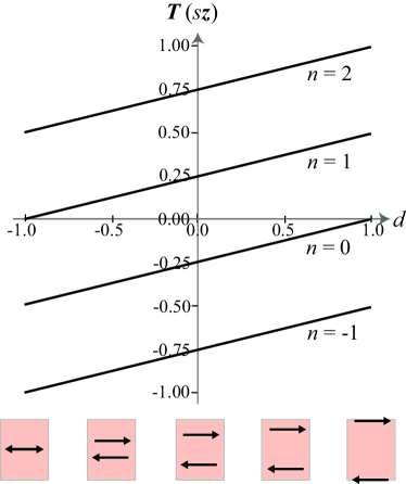
Figure 4: Allowed values of the toroidization for the antiferromagnetic chain of Fig. 3 as a function of displacement $d$ from the non-toroidal case ($d=0$). The cartoons at the bottom indicate the corresponding positions of the magnetic moments within the unit cell.

The change in toroidization between two configurations with $d=d_{1}$ and $d=d_{2}$ for a certain branch $n$ is given by:

$$\bm{T}_{n}(d_{2})-\bm{T}_{n}(d_{1})=\frac{s}{4}\left(d_{2}-d_{1}\right)\hat{\bm{z}}\quad,$$ (18)

i.e. it is independent of the branch index $n$. In particular, if the non-centrosymmetric distortion is inverted ($d_{1}=d_{0}$, $d_{2}=-d_{0})$, the change in toroidization is $2T_{\text{s}}=\frac{sd_{0}}{2}$ so that $T_{\text{s}}=\frac{sd_{0}}{4}$ can be interpreted as the spontaneous toroidization, again in analogy to the case of the electric polarization, where the spontaneous polarization is given by the branch-independent change in polarization compared to a centrosymmetric reference structure.

Another possible way to alter the toroidization is by changing the orientation of the magnetic moments instead of changing their positions. In particular, we expect that a full 180^∘ rotation of all magnetic moments, which is equivalent to the operation of time reversal, should invert the macroscopic “spontaneous toroidization”, and should therefore lead to the same change $2T_{\text{s}}$ as discussed above. If we allow the magnetic moments to rotate out of the $x$ direction, while preserving the antiparallel alignment of the two basis moments, the toroidization along the $z$ direction is given by

$$T^{z}_{n}(d,\alpha)=\left(n-\frac{1-d}{2}\right)\frac{s}{2}\cos\alpha\quad,$$ (19)

where $\alpha$ is the angle between the magnetic moments and the $x$ direction. The change in toroidization for a full 180^∘ rotation of the moments is thus:

$$T^{z}_{n}(d_{0},180^{\circ})-T^{z}_{n}(d_{0},0^{\circ})=-\frac{sd_{0}}{2}+s(2n+1)\quad,$$ (20)

and apparently depends on the branch index $n$. However, if one calculates the same change in toroidization for the non-toroidal state with $d=0$, one obtains:

$$T^{z}_{n}(0,180^{\circ})-T^{z}_{n}(0,0^{\circ})=s(2n+1)\quad.$$ (21)

Obviously, in this case the corresponding change in macroscopic toroidization should be zero, since both the initial and final states (and all intermediate states) correspond to a non-toroidal configuration and thus $T_{\text{s}}=0$. If one subtracts the improper change in $T^{z}$, Eq. (21), from the change in toroidization calculated in Eq. (20), one obtains the proper change in toroidization $2T_{\text{s}}=\frac{sd_{0}}{2}$, which is identical to one obtained by inverting the non-centrosymmetric distortion $d$. Here, we use the terminology “proper” and “improper” in analogy to the case of the proper and improper piezoelectric response, Vanderbilt (2000) where a similar branch dependence is caused by volume changes of the unit cell, and the improper piezoelectric response has to be subtracted appropriately.

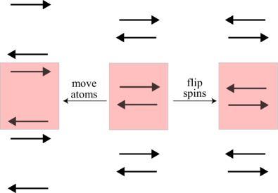
Figure 5: Effect on the magnetic moment configuration of Fig. 3b (center) of a reversal of all magnetic moments (right) and of a reversal of the non-centrosymmetric distortion $d$ (left). Note that the right and left final states are identical, with the moments on the left translated by half a unit cell compared to those on the right.

Fig. 5 shows the initial and final states for the two cases where either the moment displacements or the magnetic moment directions are inverted. The two final states are equivalent except for a translation of all moments by half a unit cell along $y$, which, again due to Neumann’s principle, is irrelevant for the macroscopic properties. The spontaneous toroidization of the state on the left in Fig. 5 is therefore the same as for the state on the right side of Fig. 5.

VI Toroidizations for some example materials

To further illustrate the concept of toroidal moments in crystalline solids and to investigate the consequences of the definitions and simplifications outlined in the preceding sections for real systems, we now evaluate the toroidizations of four example materials: BaNiF₄, LiCoPO₄, GaFeO₃, and BiFeO₃. All these materials have been discussed recently in the context of multiferroics, magneto-electric coupling, or ferrotoroidics. BaNiF₄ and BiFeO₃ are both antiferromagnetic ferroelectrics, with additional weak ferromagnetism in the case of BiFeO₃, and the possible coupling between the various order parameters in these systems has recently been studied using first principles techniques.Ederer and Spaldin (2006, 2005) LiCoPO₄, which is not ferroelectric, exhibits a rather large linear magneto-electric effect,Rivera (1994) and the observation of ferrotoroidic domains in this material using nonlinear optical techniques has been reported.Van Aken et al. (2007) GaFeO₃ is a magnetic piezoelectric which exhibits a strong asymmetry in the magneto-electric tensor. This asymmetry has been interpreted to result from a non-vanishing toroidal moment in this material.Popov et al. (1998)

VI.1 BaNiF₄

BaNiF₄ belongs to an isostructural family of antiferromagnetic ferroelectrics with composition Ba$M$F₄, where $M$ can be Mn, Fe, Co, or Ni.v. Schnering and Bleckmann (1968); Eibschütz et al. (1969) It was recently shown that BaNiF₄ exhibits two distinct antiferromagnetic order parameters and that the order parameter corresponding to the “weak” (secondary) antiferromagnetic order can be reversed by using an electric field.Ederer and Spaldin (2005) The crystallographic structure of BaNiF₄ is orthorhombic corresponding to space group $Cmc2_{1}$.v. Schnering and Bleckmann (1968); Eibschütz et al. (1969) The magnetic space group is $P_{a}2_{1}$,Cox et al. (1970) which contains a non-primitive translation along the $a$ direction combined with time inversion.Bradley and Cracknell (1972) This reflects the fact that the antiferromagnetic ordering in BaNiF₄ leads to a unit cell doubling compared to the paramagnetic phase. The corresponding (macroscopic) magnetic point group is thus $21^{\prime}$, which does not break time inversion, similar to the case of the one-dimensional antiferromagnetic chain discussed in Sec. V.1. Therefore, neither a macroscopic magnetization nor a macroscopic toroidal moment is allowed in this symmetry. We note that, in general, when the magnetic ordering leads to a unit cell doubling compared to the paramagnetic phase, then the system is always macroscopically time reversal symmetric and therefore non-toroidal.

Table 1: Positions $\bm{r}_{i}$ and moment directions $\bm{m}_{i}$ of the magnetic Ni cations in BaNiF₄. $a$, $b$ and $c$ are the orthorhombic lattice constants, $\delta$ represents an internal structural parameter, $\theta$ is the angle between the magnetic moments and the orthorhombic $b$ axis, and $S$ is the magnitude of the Ni magnetic moment. The corresponding lattice vectors are: $\bm{a}_{1}=(a,b,0)$, $\bm{a}_{2}=(a/2,-b/2,0)$, and $\bm{a}_{3}=(0,0,c)$.

site	$r^{x}_{i}/a$	$r^{y}_{i}/b$	$r^{z}_{i}/c$	$m^{x}_{i}$	$m^{y}_{i}$	$m^{z}_{i}$
Ni	0	$\delta$	0	0	$S\cos\theta$	$S\sin\theta$
Ni	0	$-\delta$	$\tfrac{1}{2}$	0	$-S\cos\theta$	$S\sin\theta$
Ni	1	$\delta$	0	0	$-S\cos\theta$	$-S\sin\theta$
Ni	1	$-\delta$	$\tfrac{1}{2}$	0	$S\cos\theta$	$-S\sin\theta$

Nevertheless it is instructive to examine the effect of the periodic boundary conditions and the resulting multivaluedness of the toroidization for this trivial case. The magnetic unit cell of BaNiF₄ contains 4 magnetic Ni ions, whose positions and spin directions are listed in Table 1. A decomposition into fully compensated and uncompensated components is not necessary, since there is no macroscopic magnetization in this system. Application of Eqs. (7) and (16) leads to a “toroidization lattice” of the form:

$$\bm{T}_{klmn}=\frac{S}{2\Omega}\left\{\cos\theta\left(\begin{array}[]{c}ck\\ 0\\ \frac{a}{2}(l-m+2n)\end{array}\right)\right.\\ \left.+\sin\theta\left(\begin{array}[]{c}\frac{b}{2}(l+m-2n)\\ \frac{b}{2}(l+m+2n+4)\\ 0\end{array}\right)\right\}\quad,$$ (22)

where $\theta$ is the canting angle of the magnetic moments (of magnitude $S$) relative to the orthorhombic $b$ direction, and $a$, $b$, $c$ are the orthorhombic lattice parameters. $k$, $l$, $m$, and $n$ are arbitrary integer numbers corresponding to four different independent toroidization increments in this system. Due to the pairwise collinear spin structure in BaNiF₄ the original $4\times 3=12$ increments according to Eq. (16) are reduced to $2\times 3=6$. Additional symmetries reduce the number of independent increments to 4. Due to the base-centered orthorhombic Bravais lattice of BaNiF₄, these toroidization increments are in general neither parallel to the cartesian coordinate directions nor perpendicular to each other. It can be seen from Eq. (22) that for a general value of the angle $\theta$, the allowed values of $\bm{T}$ do not form a Bravais lattice, and the multivaluedness of $\bm{T}$ is more complex than in the case of the electric polarization. Nevertheless, the set of allowed toroidization values in BaNiF₄ is inversion symmetric as required by the time-symmetric point group. In the absence of canting ($\theta=0^{\circ}$), the toroidization and the toroidization increment along the $b$ direction would be zero; however we see that for small $\theta$ there is a small non-zero increment of the toroidization along this direction, reflecting the small component of the magnetic moments perpendicular to $b$. Thus, the example of BaNiF₄ shows that the structure of the set of allowed toroidization values is in general more complex than the “polarization lattice” in the modern theory of electric polarization in crystalline solids.

VI.2 LiCoPO₄

The observation of ferrotoroidic domains in LiCoPO₄ using nonlinear optical techniques has been reported in Ref. Van Aken et al., 2007. LiCoPO₄ crystallizes in the olivine structure with the orthorhombic space group $Pnma$,Newnham and Redman (1965) and originally it was believed that the magnetic moments of the four Co ions in the unit cell are antiferromagnetically aligned along the orthorhombic $b$ direction.Santoro et al. (1966) This moment configuration corresponds to the magnetic space group $Pnma^{\prime}$, which contains the operation of simultaneous time and space inversion, but not the pure time and space inversion separately, and thus allows the existence of a macroscopic toroidal moment. Furthermore, the toroidal moment is required to be aligned parallel to the $c$ axis. Recently, it was found that the magnetic moments in LiCoPO₄ are rotated slightly away from the $b$ direction by an angle $\theta\approx 4.6^{\circ}$, while preserving the overall collinear magnetic structure.Vaknin et al. (2002) For a moment rotation within the $b$-$c$ plane, the rotated moment configuration corresponds to a lower symmetry with the magnetic point group $2^{\prime}/m$, which allows a toroidal moment also along the orthorhombic $b$ direction. At the moment, it is not clear what the primary order parameter for this additional symmetry lowering is, although since it does not change the relative antiferromagnetic arrangement of the spins a toroidal origin has been proposed.Van Aken et al. (2007) Furthermore, a weak magnetization has been measured along the $b$ direction,Kharchenko et al. (2001) which indicates an even lower point group symmetry of $2^{\prime}$. Since the small magnetization occurs along the $b$ direction, i.e. parallel to the direction of the antiferromagnetic alignment, it has been described as weak ferrimagnetism.

Table 2: Positions $\bm{r}_{i}$ and magnetic moment directions $\bm{m}_{i}$ of the Co cations in LiCoPO₄, according to Ref. Vaknin et al., 2002 and assuming a moment rotation towards the $c$ direction. $\epsilon$ and $\delta$ are internal structural parameters corresponding to Wyckoff positions 4$c$ of the $Pnma$ space group. $\theta$ is the angle between the magnetic moments and the $b$ axis and $S$ is the magnitude of the Co magnetic moment. Experimental values are $\epsilon=0.0286$, $\delta=0.0207$, and $\theta\approx 4.6^{\circ}$.Vaknin et al. (2002) The orthorhombic lattice parameters are $a=10.20$ Å, $b=5.92$ Å, and $c=4.70$ Å.Newnham and Redman (1965)

site	$r^{x}_{i}/a$	$r^{y}_{i}/b$	$r^{z}_{i}/c$	$m^{x}_{i}$	$m^{y}_{i}$	$m^{z}_{i}$
Co	$1/4+\epsilon$	$1/4$	$-\delta$	0	$-S\cos\theta$	$-S\sin\theta$
Co	$1/4-\epsilon$	$-1/4$	$1/2-\delta$	0	$S\cos\theta$	$S\sin\theta$
Co	$-1/4-\epsilon$	$-1/4$	$\delta$	0	$S\cos\theta$	$S\sin\theta$
Co	$-1/4+\epsilon$	$1/4$	$1/2+\delta$	0	$-S\cos\theta$	$-S\sin\theta$

Here we calculate the toroidization corresponding to the fully compensated antiferromagnetic configuration with magnetic point group $2^{\prime}/m$, where all spins are rotated from the $b$ direction towards the $c$ direction by an angle $\theta$. The corresponding positions and spin directions of the four magnetic Co cations within the unit cell are listed in Table 2. The toroidization resulting from Eqs. (7) and (16) is:

$$\bm{T}_{nml}=\frac{S}{2\Omega}\left\{\cos\theta\left(\begin{array}[]{c}cm\\ 0\\ (4\epsilon\mp l)a\end{array}\right)+\sin\theta\left(\begin{array}[]{c}bn\\ (4\epsilon\pm l)a\\ 0\end{array}\right)\right\}\quad.$$ (23)

Here, $a$, $b$ and $c$ are the orthorhombic lattice constants and $n$, $m$, and $l$ are arbitrary integer numbers. It can be seen that there is only a trivial component of $\bm{T}$ along the $a$ direction and that there is a nontrivial part of the toroidal moment proportional to $\epsilon$, which rotates from the $c$ direction for $\theta=0^{\circ}$ towards the $b$ direction for $\theta=90^{\circ}$. For $\epsilon=0$ the system is centrosymmetric and thus non-toroidal. The spontaneous toroidization is given by $T_{s}=\frac{2S\epsilon a}{\Omega}$. For the experimentally reported parameters listed in Table 2 and using the formal magnetic moment $S=3\mu_{\text{B}}$ of Co²⁺, the corresponding value is $\bm{T}_{s}=6.17\cdot 10^{-3}\mu_{\text{B}}/\textrm{\AA}^{2}(\hat{\bm{z}}\cos\theta+\hat{\bm{y}}\sin\theta)$, corresponding to a spontaneous toroidal moment per unit cell of $\bm{t}_{\text{s}}=1.75\mu_{\text{B}}\textrm{\AA}\,(\hat{\bm{z}}\cos\theta+\hat{\bm{y}}\sin\theta)$. Thus, the magnetic moment rotation described by $\theta$ results in a corresponding rigid rotation of the toroidization.

VI.3 GaFeO₃

Ga_2-xFe_xO₃ was the first material that was found to exhibit both piezoelectricity and a macroscopic magnetization.Remeika (1960) It was also the first known material with a spontaneous magnetization that simultaneously exhibits a linear magneto-electric effect.Rado (1964) The system Ga_2-xFe_xO₃ has been studied recently because of its interesting optical properties, which result from the simultaneous breaking of both space and time inversion symmetries in this material.Kubota et al. (2004); Jung et al. (2004) In addition, an asymmetry of the magneto-electric tensor has been measured and was attributed to the existence of a toroidal moment in this system.Popov et al. (1998)

The crystal structure (space group $Pc2_{1}n$) of Ga_2-xFe_xO₃ contains four inequivalent cation sites, one with tetrahedral oxygen coordination and three different octahedrally coordinated sites.Abrahams et al. (1965) The Fe cations occupy predominantly two of the octahedral sites (called Fe1 and Fe2), but there is also a sizable Fe occupation on the third octahedral site (Ga2), whereas the tetrahedral site (Ga1) is occupied mainly by Ga. The exact occupation of the various cation sites depends on the composition $x$ as well as on the preparation technique and sample history.Arima et al. (2004)

Two different magnetic structures have been proposed for this system, both of which are consistent with the magnetic space group $Pc^{\prime}2_{1}^{\prime}n$, which allows for a macroscopic magnetization along the crystallographic $c$ direction. Abrahams and Reddy originally proposed a canted antiferromagnetic structure with compensating magnetic moments within the $a$-$b$ plane and a net magnetization along $c$.Abrahams and Reddy (1964) On the other hand Arima et al. (Ref. Arima et al., 2004) recently interpreted their data in terms of a collinear ferrimagnetic configuration suggested in Ref. Delapalme, 1967, where all spins are oriented either parallel or antiparallel to the $c$ direction. In both cases, the relative orientation of the four symmetry-related magnetic moments on the Fe1 sites or the Fe2 sites, respectively, is dictated by the magnetic space group $Pc^{\prime}2_{1}^{\prime}n$.

We note that in the magnetic configuration used by Arima et al. (Ref. Arima et al., 2004) the net magnetization stems mainly from the intersite disorder; the system is a perfectly compensated antiferromagnet if (i) all Fe1 and Fe2 sites are occupied by Fe cations, (ii) there is no Fe occupation of the Ga1 and Ga2 sites, and (iii) the magnetic moments on the two Fe sites are the same. Here, we consider only this perfectly compensated configuration with no site disorder and composition $x=1$, i.e. all Fe1 and Fe2 sites are occupied by Fe³⁺ cations and all Ga1 and Ga2 sites are occupied by Ga³⁺ cations. Thus, the magnetic configuration discussed in the following does not have a net magnetization. We point out that in general the magnetic and toroidal properties will depend on the exact occupation numbers of the various cation sites. The positions of the Fe sites as well as the corresponding moment directions are listed in Table 3.

Table 3: Positions $\bm{r}_{i}$ and magnetic moment directions $\bm{m}_{i}$ of the Fe sites in GaFeO₃ with magnetic space group $Pc^{\prime}2_{1}^{\prime}n$. Both Fe sites correspond to Wyckoff positions 4$a$. The magnetic configuration is that discussed in Ref. Arima et al., 2004. $S$ is the magnitude of the Fe magnetic moment, which is assumed to be identical on both sites and $a$, $b$, $c$ are the usual orthorhombic lattice parameters.

site	$r^{x}/a$	$r^{y}/b$	$r^{z}/c$	$m_{i}^{x}$	$m_{i}^{y}$	$m_{i}^{z}$
Fe1	$x_{1}$	$y_{1}$	$z_{1}$	0	0	$S$
Fe1	$\tfrac{1}{2}-x_{1}$	$y_{1}$	$\tfrac{1}{2}+z_{1}$	0	0	$S$
Fe1	$\tfrac{1}{2}+x_{1}$	$y_{1}-\tfrac{1}{2}$	$\tfrac{1}{2}-z_{1}$	0	0	$S$
Fe1	$1-x_{1}$	$y_{1}-\tfrac{1}{2}$	$1-z_{1}$	0	0	$S$
Fe2	$x_{2}$	$y_{2}$	$z_{2}$	0	0	$-S$
Fe2	$\tfrac{1}{2}-x_{2}$	$y_{2}$	$\tfrac{1}{2}+z_{2}$	0	0	$-S$
Fe2	$\tfrac{1}{2}+x_{2}$	$y_{2}-\tfrac{1}{2}$	$\tfrac{1}{2}-z_{2}$	0	0	$-S$
Fe2	$1-x_{2}$	$y_{2}-\tfrac{1}{2}$	$1-z_{2}$	0	0	$-S$

The magnetic space group $Pc^{\prime}2_{1}^{\prime}n$ breaks both space and time reversal symmetries and thus allows the existence of a macroscopic toroidal moment. Evaluation of Eqs. (7) and (16) for the positions and moment directions listed in Table 3 leads to the toroidization:

$$\bm{T}_{nm}=\frac{S}{2\Omega}\left(\begin{array}[]{c}4(y_{1}-y_{2})b+nb\\ ma\\ 0\end{array}\right)\quad.$$ (24)

It can be seen that there is a nontrivial toroidization along the $a$ direction, as dictated by the magnetic space group symmetry, whereas the component along the $b$ direction represents only the trivial increment resulting from the periodic boundary conditions, and the component along $c$ is zero. The macroscopic toroidization along $a$ depends on the difference of the coordinates $y_{1}$ and $y_{2}$ of the two different Fe sites along $b$.

One can verify that for $y_{1}-y_{2}=\frac{1}{4}l$ (for any integer $l$) the “magnetic lattice”, i.e. the spatial arrangement of magnetic moments on the Fe1 and Fe2 sites, is centrosymmetric, and thus the system is non-toroidic in the localized moment limit (see also Ref. Arima et al., 2004). This is consistent with Eq. (24), which for $y_{1}-y_{2}=\frac{1}{4}l$ results only in a trivial non-toroidal component of $\bm{T}$ along the $a$ direction. We point out that the non-toroidicity for $y_{1}-y_{2}=\frac{1}{4}l$ holds true only for the case of localized magnetic moments, where the presence of all nonmagnetic ions is neglected. The full crystallographic symmetry of this system (given by both magnetic and nonmagnetic ions) is non-centrosymmetric even for $y_{1}-y_{2}=\frac{1}{4}l$. In fact, GaFeO₃ is an example of a pyroelectric crystal that is polar but not ferroelectric, i.e. the polarization cannot be switched, since it does not result from a small distortion of a centrosymmetric reference structure. However, in the localized moment picture the system is non-toroidal for $y_{1}-y_{2}=\frac{1}{4}l$ and we can evaluate the spontaneous toroidization with respect to this reference configuration. The relevant structural parameters determined experimentally in Ref. Arima et al., 2004 at 4 K are: $a=8.719$ Å, $b=9.368$ Å, $c=5.067$ Å, $y_{1}=0.5831$, and $y_{2}=0.7998$. This gives a spontaneous toroidization of $T_{s}=\frac{2Sb}{\Omega}(0.25-0.2167)=7.5\cdot 10^{-3}\mu_{\text{B}}/\textrm{\AA}^{2}$, corresponding to a spontaneous toroidal moment per unit cell of $3.1\mu_{\text{B}}\textrm{\AA}$. Here, we used the formal magnetic moment $S=5\mu_{\text{B}}$ of Fe³⁺.

It can be seen from Eq. (24) that the set of toroidization values is also centrosymmetric around the origin if $y_{1}-y_{2}$ is equal to any integer multiple of $\frac{1}{8}$, even though only for $y_{1}-y_{2}=\frac{1}{4}l$ the corresponding magnetic moment configuration is non-toroidal as discussed in the previous paragraph. This shows that even though the set of toroidization values of a non-toroidal structure is always centrosymmetric, the converse is not necessarily true. A centrosymmetric set of toroidization values does not necessarily correspond to a non-toroidal state. Thus, for $y_{1}-y_{2}=(2k+1)\cdot\frac{1}{8}$ the higher symmetry of the toroidization values is accidental and does not correspond to a vanishing macroscopic toroidization.

The toroidal moment of a single unit cell of GaFeO₃ was also evaluated in Ref. Popov et al., 1998, without taking into account the multivaluedness of the toroidization due to the periodic boundary conditions. A value of $t_{0}=24.155\,\mu_{B}$Å along the $a$ direction was reported for the centrosymmetric reference structure with $y_{1}-y_{2}=-0.25$, and the spontaneous toroidal moment was specified as 0.03 $t_{0}$. It is unclear from Ref. Popov et al., 1998 whether mixing of Fe ions onto the Ga sites was included in the calculation and therefore a direct comparison with our calculation is not possible.

VI.4 BiFeO₃

BiFeO₃ is a multiferroic material of high practical interest since it combines both magnetic and ferroelectric order above room temperature (see Ref. Wang et al., 2003). It exhibits a rhombohedrally distorted perovskite structure (space group $R3c$) involving both polar displacements of the ions along the [111] direction and counter-rotations of oxygen octahedra around this direction.Michel et al. (1969); Kubel and Schmid (1990); Neaton et al. (2005) The spin structure of BiFeO₃ is a superposition of various components. In a first approximation, the spins order in a G-type antiferromagnetic structure, where all neighboring magnetic moments are oriented antiparallel to each other.Fischer et al. (1980) In addition, in bulk BiFeO₃ the axis along which the spins are aligned rotates throughout the crystal, leading to an additional spiral spin structure with a large period of $\sim$620 Å.Sosnowska et al. (1982) However, this spiral component is absent in thin film samples,Bea et al. (2007) where instead a weak ferromagnetic moment, resulting from a small canting of the magnetic moments, has been reported.Wang et al. (2003); Ederer and Spaldin (2006) Here, we exclude the bulk spiral component as well as the small weakly ferromagnetic component from the discussion. Depending on the direction of the antiparallel Fe moments, the magnetic point group is either $3m$ (if the moments are aligned along the polar $z$ axis), $m$ (if the moments are oriented perpendicular to the polar axis and parallel to the glide plane), or $m^{\prime}$ (with the moments perpendicular to the glide plane); all of these symmetries allow for a macroscopic toroidization. First-principles calculations showed that $3m$ symmetry, which would not allow for a macroscopic magnetization, is energetically unfavorable.Ederer and Spaldin (2005)

BiFeO₃ provides an instructive example to illustrate the limitations of the localized moment approach to toroidal moments based on Eq. (7). Both space and time-inversion symmetries are broken in BiFeO₃, so that in principle a toroidal moment is symmetry-allowed for this system. Indeed, an antisymmetric component of the magneto-electric tensor, indicating a non-vanishing toroidal moment, has been measured at high magnetic fields where the bulk spiral spin structure is destroyed.Popov et al. (2001) However, if we consider only the localized spins on the Fe sites, the magnetic lattice is centrosymmetric, i.e. it has a higher symmetry than the full magnetization density $\bm{\mu}(\bm{r})$ (see the discussion towards the end of Sec. II), and thus the corresponding toroidal moment vanishes. In the $R3c$ crystal structure of BiFeO₃ the inversion symmetry is lifted by displacements of the different ionic sub-lattices relative to each other. Since the local moment picture neglects the presence of all nonmagnetic ions, this inversion symmetry-breaking is not present in the purely magnetic lattice.

If we take the rhombohedral axis of BiFeO₃ as the $z$-direction (hexagonal setup of the rhombohedral unit cell) and consider a perfect G-type ordering with the magnetic moments of the Fe cations along $\pm\hat{\bm{x}}$, then the calculated toroidization is:

$$\bm{T}_{n}=\frac{S}{2\Omega}\left(\begin{array}[]{c}0\\ \frac{c}{6}+n\frac{c}{3}\\ 0\end{array}\right)\quad.$$ (25)

Here, $c$ is the lattice constant of BiFeO₃ along $z$ within the hexagonal setup. The first term along the $y$ direction in Eq. (25) is the trivial half-toroidization increment, and the whole set of toroidization values is centrosymmetric, i.e. non-toroidal. This shows that it is not always sufficient to consider magnetic dipole moments localized at the sites of the magnetic cations, but that the spatial moment distribution can be very important. The exact magnetic moment density $\bm{\mu}(\bm{r})$ always reflects the full magnetic space group symmetry of the system, whereas the reduction to localized magnetic moments can result in a higher symmetry than that of the full system.

VII Summary, conclusions, and outlook

In summary we have presented a detailed study of magnetic toroidal moments in bulk periodic solids in the limit where the toroidal moment is caused by a time and space reversal symmetry breaking arrangement of localized magnetic moments. We have reviewed the basic microscopic definitions and showed that the periodic boundary conditions lead to a multivaluedness of the toroidization, which suggests that only differences in toroidization are well-defined observable quantities. We suggest that the origin dependence of the toroidal moment should be treated by decomposing the magnetic moment arrangement into a fully compensated antiferromagnetic and an uncompensated ferromagnetic component, so that only the ferromagnetic component depends on the origin. Differences in toroidization resulting from the compensated part of the moment configuration can be evaluated rather straightforwardly, if one keeps in mind the macroscopic symmetry properties of the system. We have illustrated the main concepts and difficulties in evaluating magnetic toroidization in periodic systems by first discussing the simple example of a one-dimensional antiferromagnetic chain, and we have then analyzed the toroidization for four example materials.

In addition to illustrating the general consequences of the origin dependence and the multivaluedness of the toroidal moment in periodic systems in the localized moment limit, our main conclusion is that it is important to be aware of the macroscopic symmetry properties when evaluating toroidization changes. This is particularly striking in the example of the distorted one-dimensional antiferromagnetic chain discussed in Sec.V, where the change in polarization due to a structural distortion can be calculated straightforwardly, whereas in the case of a magnetic moment reversal one has to subtract the improper toroidization change that is caused by the corresponding change in the toroidization increment. We have also shown the limitations of the local moment picture in evaluating toroidal moments in cases where the reduction to localized moments changes the symmetry of the system.

An open question, which we have not addressed in our theoretical analysis, is how the spontaneous toroidization can be measured experimentally. According to the fundamental definition of the toroidal moment, this is in principle possible by measuring the torque on a sample that is placed in an inhomogeneous magnetic field. However, either a field with a constant curl over the whole dimension of the sample has to be generated, or the effects of other multipole moments that couple to other field components have to be subtracted appropriately. To our knowledge such a measurement has not been attempted as of yet. So far, experimental evidence for toroidal moments has been based mostly on the detection of an asymmetric component of the magneto-electric tensor, but since the corresponding prefactors are not known, an absolute quantitative determination of $\bm{T}$ is not possible. Similarly, the nonlinear optical techniques used in Ref. Van Aken et al., 2007 are mostly sensitive to symmetry breaking, but are at best semi-quantitative. Overall it appears that quantitative measurements of toroidal moments are a challenging task, but in principle possible.

Finally, we comment on some aspects of toroidal moments that have been discussed in a sometimes confusing way in the literature. First, the relation between the toroidal moment and the asymmetric component of the linear magneto-electric effect, and second the outer product of the polarization with the magnetization, which has sometimes been interpreted as a toroidal moment.

From a macroscopic symmetry point of view, the symmetries which allow for a macroscopic toroidal moment are identical with that allowing for an antisymmetric component of the linear magneto-electric effect tensor. The relation between these two quantities can be seen by analyzing the following free energy expression (see also Ref. Sannikov, 1997):

$$U=\frac{1}{2}\kappa P^{2}-\bm{P}\cdot\bm{E}+\frac{1}{2}BM^{2}-\bm{M}\cdot\bm{H}\\ +\frac{1}{2}AT^{2}+\frac{1}{4}CT^{4}+a\bm{T}\cdot\left(\bm{P}\times\bm{M}\right)\quad.$$ (26)

This is the simplest possible free energy expression that can simultaneously describe (i) a phase transition from a para-toroidic ($T=|\bm{T}|=0$) into a ferrotoroidic phase ($T\neq 0$), (ii) the coupling of the electric polarization $\bm{P}$ and the magnetization $\bm{M}$ to the electric field $\bm{E}$ and the magnetic field $\bm{H}$, respectively, and (iii) a coupling between the electric polarization, the magnetization, and the toroidization. In Eq. (26) $\kappa$ and $B$ are the inverse electric and magnetic susceptibilities, $A$ and $C$ are temperature dependent coefficients, and $a$ determines the strength of the magneto-electric coupling. The trilinear form of the coupling term in Eq. (26) is the lowest possible order that is compatible with the overall space and time reversal symmetries. The equilibrium values for $\bm{P}$ and $\bm{M}$ can be obtained by minimizing Eq. (26). This leads to:

$$\bm{P}=\frac{1}{\kappa}\left\{\bm{E}-a(\bm{M}\times\bm{T})\right\}$$ (27)

and

$$\bm{M}=\frac{1}{B}\left\{\bm{H}-a(\bm{T}\times\bm{P})\right\}\quad.$$ (28)

If one inserts Eq. (28) into Eq. (27) one obtains (to leading order in $\bm{T}$):

$$\bm{P}=\frac{1}{\kappa}\bm{E}-\frac{a}{\kappa B}(\bm{H}\times\bm{T})\quad.$$ (29)

The last term in Eq. (29) represents an antisymmetric linear magneto-electric effect proportional to the toroidization. Thus, the presence of the trilinear coupling term between toroidization, magnetization, and polarization in Eq. (26) gives rise to an antisymmetric magneto-electric effect $\bm{P}=\alpha\bm{H}$ in the ferrotoroidic phase, with $\alpha_{ij}=-\frac{a}{\kappa B}\sum_{k}\epsilon_{ijk}T_{k}$. Note that in general other terms in the free-energy expansion can give rise to additional symmetric contributions to the magneto-electric tensor, which are not proportional to the toroidal moment.

In Eq. (26) only the magnetization and the polarization couple to $\bm{H}$ and $\bm{E}$, the toroidization in general does not couple to any homogeneous external fields, in agreement with the fundamental definitions discussed in Sec. II (in particular Eq. (3)). The effective coupling represented by the invariant $E_{\text{ME}}\sim\bm{T}\cdot(\bm{E}\times\bm{H})$ (discussed in Refs. Dubovik and Tugushev, 1990; Gorbatsevich and Kopaev, 1994; Schmid, 2003) arises from the trilinear coupling term in Eq. (26) if $\bm{P}$ and $\bm{M}$ are substituted by their corresponding fields, by inserting Eqs. (27) and (28) into Eq. (26). Of course it depends on the problem at hand whether it is more convenient to use the fields $\bm{E}$ and $\bm{H}$ or the magnetization $\bm{M}$ and polarization $\bm{P}$ as free variables. It is worth pointing out, though, that the two cases should be carefully distinguished. One can either use a description where $\bm{P}$, $\bm{T}$, and $\bm{M}$ are the free variables, $\bm{P}$ and $\bm{M}$ couple linearly to their corresponding fields, and there is a trilinear coupling term of the form $\bm{T}\cdot(\bm{P}\times\bm{M})$, or one can alternatively use a picture where the variables $\bm{P}$ and $\bm{M}$ are eliminated altogether and are replaced by the field variables $\bm{E}$ and $\bm{H}$. In this case the trilinear coupling term leads to an effective coupling of $\bm{T}$ to $\bm{E}\times\bm{H}$.

Another source of confusion is the relation of the toroidization to the cross product $\bm{P}\times\bm{M}$, which has the same time and space reversal symmetry as $\bm{T}$. This has led to a number of instances in the literature in which $\bm{P}\times\bm{M}$ itself has been described as a “toroidal moment”.Arima et al. (2005); Sawada and Nagaosa (2005); Yamasaki et al. (2006) We point out that this is generally not correct. From our discussion in Sec. III it becomes clear that $\bm{P}\times\bm{M}$ can never describe a toroidal moment resulting from the compensated part of a magnetic moment configuration (for which $\bm{M}=0$). We have also shown in Sec. III that the change in toroidal moment resulting from the uncompensated part of the magnetic moment configuration can be expressed as $\Delta\tilde{\bm{t}}=1/2\Delta\bar{\bm{R}}\times\bm{m}$, where $\Delta\bar{\bm{R}}$ is the average (non-centrosymmetric) displacement of the magnetic moments. We point out that, at least in the localized moment picture, $\Delta\bar{\bm{R}}$ is in general not proportional to $\bm{P}$, and therefore the toroidal moment is in general not proportional to $\bm{P}\times\bm{M}$. In most magnetic ferroelectrics, the polarization is related to a rigid shift of the magnetic cations relative to the non-magnetic ions, which does not affect the average position $\bar{\bm{R}}$ of the magnetic cations. It is therefore not clear whether the conditions for $\bm{T}\sim\bm{P}\times\bm{M}$ are fulfilled in any currently known material.

It has been argued that ferrotoroidicity is a key concept for fitting all forms of ferroic order in a simple fundamental scheme based on the different transformation properties of the corresponding order parameters with respect to time and space inversion (see Refs. Schmid, 2003, 2004; Van Aken et al., 2007, in particular Fig. 2 in Ref. Van Aken et al., 2007). The four fundamental forms of ferroic order listed in these references are ferroelasticity, ferroelectricity, ferromagnetism, and ferrotoroidicity, with order parameters transforming according to the four different representations of the “parity group”, which is generated by the two operations of time and space reversal.Ascher (1974) A similar scheme has also been proposed in Ref. Dubovik and Tugushev, 1990, but with the electric toroidal moment $\bm{g}$ (see Sec. I and also Refs. Naumov et al., 2004; Prosandeev et al., 2006) as the time and space symmetric order parameter instead of the ferroelastic strain tensor. The latter classification scheme seems more natural to us, since in this case all ferroic order parameters are vector quantities. It is thus very important to clearly distinguish between magnetic ferrotoroidicity and electric ferrotoroidicity, which correspond to different representations of the parity group. On the other hand, the existence of ferroelasticity, with the second-rank strain tensor as time and space invariant order parameter, raises the question, whether other ferroic second-rank tensor order parameters, corresponding to different representations of the parity group, can be identified in the future.