Energy Density-Flux Correlations
in an Unusual Quantum State and in the Vacuum

Abstract

In this paper we consider the question of the degree to which negative and positive energy are intertwined. We examine in more detail a previously studied quantum state of the massless minimally coupled scalar field, which we call a “Helfer state”. This is a state in which the energy density can be made arbitrarily negative over an arbitrarily large region of space, but only at one instant in time. In the Helfer state, the negative energy density is accompanied by rapidly time-varying energy fluxes. It is the latter feature which allows the quantum inequalities, bounds which restrict the magnitude and duration of negative energy, to hold for this class of states. An observer who initially passes through the negative energy region will quickly encounter fluxes of positive energy which subsequently enter the region. We examine in detail the correlation between the energy density and flux in the Helfer state in terms of their expectation values. We then study the correlation function between energy density and flux in the Minkowski vacuum state, for a massless minimally coupled scalar field in both two and four dimensions. In this latter analysis we examine correlation functions rather than expectation values. Remarkably, we see qualitatively similar behavior to that in the Helfer state. More specifically, an initial negative energy vacuum fluctuation in some region of space is correlated with a subsequent flux fluctuation of positive energy into the region. We speculate that the mechanism which ensures that the quantum inequalities hold in the Helfer state, as well as in other quantum states associated with negative energy, is, at least in some sense, already “encoded” in the fluctuations of the vacuum.

I Introduction

It has been known for quite some time that quantum field theories generically contain states associated with negative energy EGJ . Indeed, negative energy seems to be required by the laws of physics for such effects as Hawking evaporation (which allows the unification of black holes with the laws of thermodynamics) H75 , and for the stability of the Minkowski vacuum. In the former case, the positive Hawking radiation observed at infinity is paid for by a flux of negative energy down the horizon of the black hole DFUC . In the latter case, since the vacuum is not an eigenstate of energy density, there will be energy density fluctuations in the vacuum. In order for the averaged energy density to be zero, there must exist negative, as well as positive, energy density vacuum fluctuations. States associated with negative energy are now routinely produced in the laboratory, e.g, squeezed vacuum states and the Casimir effect SY ; C . However, the energy density itself is too small to be directly measurable.

On the other hand, unrestricted amounts of negative energy could result in gross macroscopic effects such as violation of the second law of thermodynamics F78 ; F91 , and exotic spacetime geometries such as wormholes MT ; MTY , warp drives A ; PFWD ; ER ; K98 , and time machines H92 . However, the laws of quantum field theory contain restrictions on negative energy in the form of “quantum inequalities”. These involve bounds on the magnitude of negative energy and on its temporal or spatial extent. There has been much progress in this area in the last 15 years (for some recent reviews see Refs. TR-MGM10 ; CJF-Rev ; LF100 ).

Some years ago, Helfer Helfer96 suggested the existence of a class of quantum states in which one could make the energy density arbitrarily negative in an arbitrarily large region of space, even in Minkowski spacetime. We call these “Helfer states.” The present authors, together with Helfer, verified this claim in an earlier paper FHR , which we will refer to as FHR. In that paper the characteristics of the energy density were analyzed. We argued that a crucial feature of these states is the fact that although the energy density can be made arbitrarily negative over an arbitrarily large region of space, this can be done only at one instant of time. The worldline quantum inequalities must hold for these states as well, since they have been proven to hold for all quantum states. Therefore, for this to be true, there must be rapidly time-varying fluxes which accompany the negative energy density. In the current paper, we show that this is indeed the case. The expectation values of the energy density and flux in a particular Helfer state are calculated and graphed, and their correlations are studied. An inertial observer who initially passes through the negative energy region must quickly encounter fluxes of positive energy which subsequently enter the region, thus ensuring that the time-averaged sampled energy density along the observer’s worldline is non-negative, in accordance with the quantum inequalities.

These fascinating correlations of flux and energy density are by no means unique to the Helfer states. In the second part of the paper we calculate the energy density-flux correlation function for the Minkowski vacuum state, in both two and four-dimensional spacetime. Although here we analyze correlation functions, as opposed to expectation values, nonetheless, we find remarkably similar behavior for the fluctuations of energy density and flux in the vacuum to their expectation values in the Helfer states. An initial negative energy vacuum fluctuation in some region of space is correlated with a subsequent flux fluctuation of positive energy into the region. We speculate that the mechanism which ensures that the quantum inequalities hold in the Helfer state, as well as in other quantum states associated with negative energy, is, at least in some sense, already “encoded” in the fluctuations of the vacuum.

II The Helfer State

Here we briefly summarize the results of FHR, and refer the reader to that paper for more details. The quantum state used in FHR is a superposition of two-particle states, which can be expressed as

$$|\psi\rangle=N\left[|0\rangle+\int d^{3}k_{1}\,d^{3}k_{2}\,b({\bf k}_{1},{\bf k}_{2})\,|{{\bf k}_{1},{\bf k}_{2}}\rangle\right]\,,$$ (1)

where the two-particle state, $|{{\bf k}_{1},{\bf k}_{2}}\rangle$, contains particles with three-momenta ${\bf k}_{1}$ and ${\bf k}_{2}$. The normalization factor $N$ is given by

$$N=\left[1+2\int d^{3}k_{1}\,d^{3}k_{2}\,|b({\bf k}_{1},{\bf k}_{2})|^{2}\right]^{-\frac{1}{2}}\,.$$ (2)

We consider the case where

$$b({\bf k}_{1},{\bf k}_{2})=\chi({\bf k}_{1}+{\bf k}_{2})\,(|{\bf k}_{1}||{\bf k}_{2}|)^{-1}\,,$$ (3)

and

$$\chi({\bf p})=\left\{\begin{array}[]{ll}\chi_{0}\,,&\mbox{if $|{\bf p}|\leq p_{0}$}\\ 0\,,&\mbox{otherwise}\end{array}\right.$$ (4)

where $\chi_{0}$ and $p_{0}$ are arbitrary constants, and ${\bf p}={\bf k}_{1}+{\bf k}_{2}$. (This is the $\nu=-1/2$ limit of the state discussed in FHR.) In addition, we require that the magnitudes of the momenta of the particles be less than a cutoff parameter, $\Lambda$, so that $|{\bf k}_{1}|,|{\bf k}_{2}|<\Lambda$. Thus, the state is described by the three parameters, $\Lambda$, $\chi_{0}$, and $p_{0}$. In the limit that $\Lambda$ becomes large, with $\chi_{0}$ and $p_{0}$ fixed, the two members of the pair of particles have nearly opposite momenta. This is the limit of particular interest.

II.1 Energy Density in the Helfer State

The energy density of a massless, minimally coupled scalar field may be obtained from the renormalized two-point function using

$$\rho=\frac{1}{2}\lim_{{{\bf x^{\prime}}\rightarrow{\bf x}}\atop{t^{\prime}\rightarrow t}}\left[(\partial_{t}\partial_{t^{\prime}}+\mbox{\boldmath$\nabla\cdot\nabla^{\prime}$})\,\langle:\varphi(x)\,\varphi(x^{\prime}):\rangle\right]\,.$$ (5)

Units in which $\hbar=c=1$ are used throughout this paper. In our case, this two-point function may be shown to be

$$\langle:\varphi(x)\,\varphi(x^{\prime}):\rangle = \frac{2N^{2}}{(2\pi)^{3}}\,{\rm Re}\int d^{3}k\,d^{3}k^{\prime}\,\frac{1}{\sqrt{\omega\omega^{\prime}}}\,$$ (6)

$$\times \Bigl{[}2{\rm e}^{i({\bf k^{\prime}}\cdot{\bf x^{\prime}}-{\bf k}\cdot{\bf x})}{\rm e}^{i(\omega\,t-\omega^{\prime}\,t^{\prime})}\,\int d^{3}k_{1}b^{*}({\bf k}_{1},{\bf k})b({\bf k}_{1},{\bf k^{\prime}})$$

$$+ {\rm e}^{i({\bf k}\cdot{\bf x}+{\bf k^{\prime}}\cdot{\bf x^{\prime}})}{\rm e}^{-i(\omega\,t+\omega^{\prime}\,t^{\prime})}\,b({\bf k},{\bf k^{\prime}})\Bigr{]}\,.$$

The resulting energy density is

$$\rho = \frac{N^{2}}{(2\pi)^{3}}\,{\rm Re}\int d^{3}k\,d^{3}k^{\prime}\,\sqrt{\omega\omega^{\prime}}\,(1+\hat{{\bf k}}\cdot\hat{{\bf k}}^{\prime})\,\Bigl{[}2{\rm e}^{i({\bf k^{\prime}}-{\bf k})\cdot{\bf x}}{\rm e}^{i(\omega-\omega^{\prime})t}\,\int d^{3}k_{1}b^{*}({\bf k}_{1},{\bf k})b({\bf k}_{1},{\bf k^{\prime}})$$ (7)

$$\,\,\,\,-{\rm e}^{i({\bf k}+{\bf k^{\prime}})\cdot{\bf x}}{\rm e}^{-i(\omega+\omega^{\prime})t}\,b({\bf k},{\bf k^{\prime}})\Bigr{]}\,,$$

where $\hat{{\bf k}}$ and $\hat{{\bf k}}^{\prime}$ are unit vectors in the directions of ${\bf k}$ and ${\bf k^{\prime}}$, respectively. It is convenient to write $\rho=\rho_{1}+\rho_{2}$, where $\rho_{1}$ is the contribution quadratic in $b$, and $\rho_{2}$ is that linear in $b$.

In general, it is difficult to evaluate $\rho$ explicitly for the choice of $b({\bf k}_{1},{\bf k}_{2})$ given by Eqs. (3) and (4). However, in FHR approximate forms were derived in the limit that the dominant contribution comes from modes whose frequency is large compared to $p_{0}$, which is expected to be the case when $\Lambda\gg p_{0}$. These approximate forms contain an undetermined constant $q\gg 1$ which is introduced by making a lower cutoff in the $\omega$-integrals of $qp_{0}$. The result for $\rho_{2}$ is

$$\rho_{2}\approx-\frac{\chi_{0}N^{2}}{6\pi^{2}}\,f_{2}(p_{0},r)\,\int_{qp_{0}}^{\Lambda}d\omega\,\omega^{-1}\,\cos(2\omega t)\,,$$ (8)

where

$$f_{2}(p_{0},r)=\frac{4\pi}{r^{5}}\,[3(p_{0}^{2}r^{2}-2)\sin(p_{0}r)-p_{0}r(p_{0}^{2}r^{2}-6)\cos(p_{0}r)]\,.$$ (9)

The function $f_{2}(p_{0},r)$ has the following behavior:

$$f_{2}(p_{0},r)\sim\left\{\begin{array}[]{ll}-(4\pi/r^{2})\,{p_{0}}^{3}\,{\rm cos}\,p_{0}r\,,&\mbox{$r\gg{p_{0}}^{-1}$}\\ (4\pi/5)\,p_{0}^{5}\,,&\mbox{$r\ll{p_{0}}^{-1}$}\end{array}\right.\,.$$ (10)

At $t=0$, Eq. (8) becomes

$$\rho_{2}\approx-\frac{\chi_{0}N^{2}}{6\pi^{2}}\,f_{2}(p_{0},r)\,\ln\left(\frac{\Lambda}{qp_{0}}\right)\,.$$ (11)

Let us now examine the behavior of $\rho_{1}$. From Eq. (33) of FHR, we have that

$$\rho_{1} = \frac{2\,{\chi_{0}}^{2}\,N^{2}}{(2\pi)^{3}}\,{\rm Re}\int d^{3}k_{1}\,{|k_{1}|}^{-2}\,\int_{|{\bf p}|\leq p_{0}}d^{3}p\,\int_{|{\bf p}^{\prime}|\leq p_{0}}d^{3}p^{\prime}\,(1+\hat{{\bf k}}\cdot\hat{{\bf k}}^{\prime})\,$$

$$\times{|{\bf p}-{\bf k}_{1}|}^{-1/2}\,{|{\bf p}^{\prime}-{\bf k}_{1}|}^{-1/2}\,{\rm e}^{-i({\bf p}-{\bf p}^{\prime})\cdot{\bf x}}\,{\rm e}^{i[(|{\bf p}-{\bf k}_{1}|-|{\bf p}^{\prime}-{\bf k}_{1}|)t]}\,,$$ (12)

where ${\bf p}={\bf k}_{1}+{\bf k}$ and ${\bf p}^{\prime}={\bf k}_{1}+{\bf k}^{\prime}$. In the high frequency limit, $\rho_{1}$ at $t=0$ is given by

$$\rho_{1}\approx\frac{2\,{\chi_{0}}^{2}N^{2}}{\pi^{2}}\,f_{1}(p_{0},r)\,\ln\left(\frac{\Lambda}{qp_{0}}\right)\,,$$ (13)

where

$$f_{1}(p_{0},r)\equiv\frac{{(4\pi)}^{2}}{r^{6}}\,{[\sin(p_{0}r)-p_{0}r\,\cos(p_{0}r)]}^{2}\,,$$ (14)

and

$$f_{1}(p_{0},r)\sim\left\{\begin{array}[]{ll}{(4\pi p_{0})}^{2}/r^{4}\,{\rm cos}^{2}\,(p_{0}r)\,,&\mbox{$r\gg{p_{0}}^{-1}$}\\ {(4\pi/3)}^{2}\,p_{0}^{6}\,,&\mbox{$r\ll{p_{0}}^{-1}$}\end{array}\right.\,.$$ (15)

The time dependence of $\rho_{1}$ is given by the factor of ${\rm e}^{i[(|{\bf p}-{\bf k}_{1}|-|{\bf p}^{\prime}-{\bf k}_{1}|)t]}$ in Eq. (12). In the high frequency limit,

$$|{\bf p}-{\bf k}_{1}|=k_{1}\,\sqrt{1-2\frac{{\bf p}\cdot{\bf\hat{k}}_{1}}{k_{1}}+\frac{p^{2}}{k_{1}^{2}}}\approx k_{1}-{\bf p}\cdot{\bf\hat{k}}_{1}\,,$$ (16)

where $k_{1}=|{\bf k}_{1}|$. As a result,

$$\omega-\omega^{\prime}=|{\bf p}-{\bf k}_{1}|-|{\bf p}^{\prime}-{\bf k}_{1}|\approx{\bf\hat{k}}_{1}\cdot({\bf p}^{\prime}-{\bf p})\,.$$ (17)

Because $|{\bf p}|,|{\bf p}^{\prime}|\leq p_{0}$, the time dependence of $\rho_{1}$ is on a time scale of order $1/p_{0}$, and can be neglected if we are interested only in times for which $|t|\ll 1/p_{0}$. The time variation of the regions of negative energy is governed by the rapid time dependence of $\rho_{2}$ coming from the $\cos(2\omega t)$ factor in Eq. (8). This is the time variation which allows the quantum inequalities to be satisfied in this case.

The integral in the normalization factor, Eq. (2), is

$$I=\chi_{0}^{2}\,\int d^{3}k\,\int_{|{\bf p}|\leq p_{0}}d^{3}p\,(|{\bf k}||{\bf k-p}|)^{-2}\,,$$ (18)

where ${\bf k}={\bf k}_{1}$ and ${\bf p}={\bf k}_{1}+{\bf k}_{2}$. In the limit where $|{\bf k}_{1}|\gg p_{0}$, $(|{\bf k}||{\bf k-p}|)^{-2}\approx|{\bf k}|^{-4}$, so we can write

$$I\approx\chi_{0}^{2}\,\int d^{3}k\,|{\bf k}|^{-4}\,\int_{|{\bf p}|\leq p_{0}}d^{3}p\,=4\pi\chi_{0}^{2}\int_{qp_{0}}^{\Lambda}\,\omega^{-2}\,d\omega\,\int_{|{\bf p}|\leq p_{0}}d^{3}p=\frac{16\pi^{2}}{3}\chi_{0}^{2}\,\biggl{(}\frac{{p_{0}}^{2}}{q}-\frac{{p_{0}}^{3}}{\Lambda}\biggr{)}\,.$$ (19)

When $\Lambda\gg qp_{0}$, this becomes

$$I\approx\frac{16\pi^{2}}{3}\chi_{0}^{2}\,\frac{{p_{0}}^{2}}{q}\,,$$ (20)

which leads to

$$N\approx{\biggr{(}1+\frac{32\pi^{2}}{3}\chi_{0}^{2}\,\frac{{p_{0}}^{2}}{q}\biggr{)}}^{-1/2}\,.$$ (21)

For any value of $p_{0}$, the energy density is approximately constant in space over a region of size, $r\lesssim{p_{0}}^{-1}$. In this region, $(f_{2}/f_{1})\approx 9/(20\,\pi\,p_{0})$. If we choose

$$\chi_{0}<\frac{3}{80\,\pi\,p_{0}}\,,$$ (22)

then $|\rho_{2}|/\rho_{1}>1$ and hence $\rho<0$ in this region. In the limit that $\Lambda\rightarrow\infty$, we can make $\rho$ arbitrarily negative in this region. Furthermore, by making $p_{0}$ small, we can make this region arbitrarily large. Note that if Eq. (22) is satisfied, and if $q\gg 1$, then $N\approx 1$. In this case, the unknown parameter $q$ and the cutoff parameter $\Lambda$ only appear in the energy density in the ratio $\Lambda/q$. Thus we can now take this ratio to be the effective cutoff.

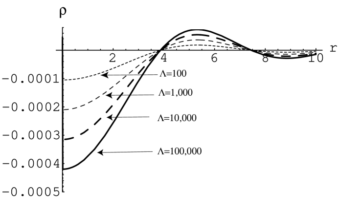
Figure 1: The total energy density $\rho=\rho_{1}+\rho_{2}$, is plotted as a function of $r$, at $t=0$, for varying $\Lambda$. We have chosen $p_{0}=1$ and $q=10$. The energy density becomes more negative with increasing $\Lambda$. Note that on scales where $r\lesssim{p_{0}}^{-1}=1$, the energy density is approximately constant and negative. Such a region may be made as large as one likes by decreasing $p_{0}$.

For the purpose of plotting the energy density, we let $q=10$ and set

$$\chi_{0}=\frac{3}{800\,\pi\,p_{0}}\,,$$ (23)

which ensures that there is a region of negative energy about $r=0$. In Fig. 1, we show the energy density as a function of $r$ at $t=0$ for several values of $\Lambda$. In Fig. 2, we illustrate the energy density for one choice of $\Lambda$ at several values of $t$ as functions of $r$. The special feature of this quantum state is that it exhibits large negative energy density at $t=0$, but this negative energy rapidly disappears, as required by the quantum inequalities. The time scale for this change is small compared to the light travel time across the negative energy region. This will be discussed in more detail in the next subsection, where we show that this rapid change in $\rho$ is associated with large energy fluxes.

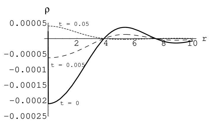
Figure 2: The total energy density $\rho=\rho_{1}+\rho_{2}$, as a function of $r$, for varying $t$. We have chosen $\Lambda=1000$, $p_{0}=1$ and $q=10$. At $t=0$ the energy density in the region near $r=0$ is negative. By $t=0.005$, it has become substantially less negative, and by $t=0.05$ it has already become positive.

II.2 The Energy Flux in the Helfer State

Let us temporarily switch to Cartesian coordinates. Then in the $z$-direction we have

$$\langle T_{0z}\rangle=-\langle T^{0z}\rangle=\frac{1}{2}\,\lim_{{{\bf x^{\prime}}\rightarrow{\bf x}}\atop{t^{\prime}\rightarrow t}}\left[(\partial_{t}\partial_{z^{\prime}}+\partial_{t^{\prime}}\partial_{z})\,\langle:\varphi(x)\,\varphi(x^{\prime}):\rangle\right]\,.$$ (24)

Using Eq. (6), we obtain

$$\langle T_{0z}\rangle=I_{1}+I_{2}\,,$$ (25)

where

$$I_{2}=\frac{N^{2}}{(2\pi)^{3}}\,{\rm Re}\int d^{3}k\,\int d^{3}k^{\prime}_{1}\,\frac{(\omega{k^{\prime}}_{z}+\omega^{\prime}{k}_{z})}{\sqrt{\omega\omega^{\prime}}}\,{\rm e}^{i({\bf k^{\prime}}+{\bf k})\cdot{\bf x}}{\rm e}^{-i(\omega+\omega^{\prime})t}\,b({\bf k},{\bf k^{\prime}})\,,$$ (26)

and

$$I_{1} = -\frac{2N^{2}}{(2\pi)^{3}}\,{\rm Re}\int d^{3}k\,\int d^{3}k^{\prime}\,\frac{(\omega{k^{\prime}}_{z}+\omega^{\prime}{k}_{z})}{\sqrt{\omega\omega^{\prime}}}\,{\rm e}^{i({\bf k^{\prime}}-{\bf k})\cdot{\bf x}}{\rm e}^{i(\omega-\omega^{\prime})t}\,$$ (27)

$$\times \,\int d^{3}k_{1}b({\bf k}_{1},{\bf k})b({\bf k}_{1},{\bf k^{\prime}})\,.$$

In the last expression, we use the fact that $b({\bf k},{\bf k^{\prime}})$ is real. At $t=0$, we have

$$I_{1}(t=0) = -\frac{2N^{2}}{(2\pi)^{3}}\,\int d^{3}k\,\int d^{3}k^{\prime}\,\frac{(\omega{k^{\prime}}_{z}+\omega^{\prime}{k}_{z})}{\sqrt{\omega\omega^{\prime}}}\,\cos[({\bf k^{\prime}}-{\bf k})\cdot{\bf x}]\,$$ (28)

$$\times \,\int d^{3}k_{1}b({\bf k}_{1},{\bf k})b({\bf k}_{1},{\bf k^{\prime}})\,.$$

However, $I_{1}(t=0)=0$, as may be seen by making the replacements ${\bf k}\rightarrow-{\bf k}$, ${\bf k}^{\prime}\rightarrow-{\bf k}^{\prime}$, and ${\bf k}_{1}\rightarrow-{\bf k}_{1}$ and using the fact that $b({\bf k}_{1},{\bf k})=b(-{\bf k}_{1},-{\bf k})$. We can see from Eq. (17) that $I_{1}$ will only vary on a time scale of order $1/p_{0}$, as does $\rho_{1}$. Thus, if we are interested in times close to $t=0$, we may set $I_{1}\approx 0$.

Next we proceed as in FHR and examine $I_{2}$. Using ${\bf p}={\bf k}+{\bf k^{\prime}}$, and taking the limit in which $\omega$ becomes large compared to $p_{0}$, we can expand the prefactor in $I_{2}$ as follows:

$$\frac{(\omega{k^{\prime}}_{z}+\omega^{\prime}{k}_{z})}{\sqrt{\omega\omega^{\prime}}} = \sqrt{|{\bf k}|\,|{\bf p}-{\bf k}|}\,\left[\frac{({\bf p}-{\bf k})\cdot\hat{\bf z}}{\sqrt{({\bf p}-{\bf k})\cdot({\bf p}-{\bf k})}}+\hat{\bf k}\cdot\hat{\bf z}\right]$$ (29)

$$= \sqrt{|{\bf k}|\,|{\bf p}-{\bf k}|}\,\left[\left(\frac{p_{z}}{\omega}-\hat{\bf k}\cdot\hat{\bf z}\right)\left(1-\frac{2\,\hat{{\bf k}}\cdot{\bf p}}{\omega}+\frac{p^{2}}{\omega^{2}}\right)^{-\frac{1}{2}}+\hat{\bf k}\cdot\hat{\bf z}\right]$$

$$\approx p_{z}-(\hat{\bf k}\cdot{\bf p})\hat{k}_{z}+\cdots\,,$$

where $\hat{k}_{z}\equiv\hat{\bf k}\cdot\hat{\bf z}$. So we can now write the integral $I_{2}$ as

$$I_{2}\approx\frac{\chi_{0}N^{2}}{(2\pi)^{3}}\,{\rm Re}\int d^{3}k\,\int_{|{\bf p}|\leq p_{0}}d^{3}p\,[p_{z}-(\hat{\bf k}\cdot{\bf p})\hat{k}_{z}]\,{\rm e}^{i{\bf p}\cdot{\bf x}}\,\,\omega^{-2}\,{\rm e}^{-2i\omega t}\,.$$ (30)

Now let

$$I_{2}=I_{2a}+I_{2b}\,,$$ (31)

where

$$I_{2a}\equiv\frac{\chi_{0}N^{2}}{(2\pi)^{3}}\,{\rm Re}\int d^{3}k\,\int_{|{\bf p}|\leq p_{0}}d^{3}p\,\,p_{z}\,{\rm e}^{i{\bf p}\cdot{\bf x}}\,\,\omega^{-2}\,{\rm e}^{-2i\omega t}$$ (32)

and

$$I_{2b}\equiv-\frac{\chi_{0}N^{2}}{(2\pi)^{3}}\,{\rm Re}\int d^{3}k\,\int_{|{\bf p}|\leq p_{0}}d^{3}p\,\,(\hat{\bf k}\cdot{\bf p})\hat{k}_{z}\,{\rm e}^{i{\bf p}\cdot{\bf x}}\,\,\omega^{-2}\,{\rm e}^{-2i\omega t}\,.$$ (33)

First let us evaluate $I_{2a}$. Performing the angular integrations, we have

$$\int d^{3}k=4\pi\int d\omega\,\omega^{2}$$ (34)

and

$$I^{\prime}_{2a}\equiv\int_{|{\bf p}|\leq p_{0}}d^{3}p\,\,p_{z}\,{\rm e}^{i{\bf p}\cdot{\bf x}}=\int_{|{\bf p}|\leq p_{0}}d^{3}p\,\,p_{z}\,{\rm e}^{ipr{\rm cos}\theta}\,,$$ (35)

where $r=|{\bf x}|$ and $\theta$ is the angle between $\bf x$ and $\bf p$.

We are assuming spherical symmetry, so let us choose, without loss of generality, $\bf x$ to point along the $z$-axis. Then $p_{z}={\bf p}\cdot{\hat{\bf z}}=p\,{\rm cos}\theta$, where $p=|{\bf p}|$. We can now write

$$I^{\prime}_{2a}=\int_{|{\bf p}|\leq p_{0}}d^{3}p\,\,p_{z}\,{\rm e}^{ipr{\rm cos}\theta}\ =2\pi\int_{0}^{p_{0}}dp\,p^{3}\int_{-1}^{1}dc\,c\,{\rm e}^{iprc}=-i\,g_{2}(p_{0},r)\,,$$ (36)

where $c=\cos\theta$ and

$$g_{2}(p_{0},r)=\frac{4\pi}{r^{4}}\,[3p_{0}r\,{\rm cos}(p_{0}r)+({p_{0}}^{2}r^{2}-3)\,{\rm sin}(p_{0}r)]\,.$$ (37)

Therefore $I_{2a}$ becomes

$$I_{2a}=-\frac{\chi_{0}N^{2}}{(2\pi)^{2}}\,g_{2}(p_{0},r)\int_{qp_{0}}^{\Lambda}d\omega\,\sin(2\omega t)\,,$$ (38)

where as before, $q$ is a constant chosen so that the approximations made in finding the integrand ($\omega\gg p_{0}$) are valid throughout the range of integration. Evaluating the integral we have

$$I_{2a}=\frac{\chi_{0}N^{2}}{4\pi^{2}}\,g_{2}(p_{0},r)\left[\frac{{\rm cos}(2\Lambda t)-{\rm cos}(2qp_{0}t)}{t}\right]\,.$$ (39)

We now turn our attention to $I_{2b}$. First fix the direction of ${\bf p}$ and integrate over the directions of ${\bf k}$. In a right-handed $x,y,z$ coordinate system, define: $\theta^{\prime}$ to be the angle between $\bf k$ and the $z$-axis, $\theta$ to be the angle between $\bf p$ and the $z$-axis, $\phi^{\prime}$ to be the azimuthal angle in the $x,y$ plane for $\bf k$, $\phi$ to be the azimuthal angle in the $x,y$ plane for $\bf p$, and $\gamma$ to be the angle between $\bf k$ and $\bf p$. Then we have that ${\hat{k}}_{z}={\bf\hat{k}}\cdot{\bf\hat{z}}={\rm cos}\theta^{\prime},{\bf\hat{k}}\cdot{\bf p}=|{\bf p}|\,{\rm cos}\gamma$, and ${\bf p}\cdot{\bf x}=p\,r\,{\rm cos}\theta$. Making use of the fact that Jackson

$${\rm cos}\gamma={\rm cos}\theta\,{\rm cos}\theta^{\prime}+{\rm sin}\theta\,{\rm sin}\theta^{\prime}\,{\rm cos}(\varphi-\varphi^{\prime})\,,$$ (40)

we can write

$$I_{2b} = -\frac{\chi_{0}N^{2}}{(2\pi)^{3}}\,{\rm Re}\int_{|{\bf p}|\leq p_{0}}d^{3}p\,\,{\rm e}^{i{\bf p}\cdot{\bf x}}\,\int d^{3}k\,p\,{\rm cos}\gamma\,{\rm cos}\theta^{\prime}\,\,\omega^{-2}\,{\rm e}^{-2i\omega t}$$ (41)

$$= -\frac{\chi_{0}N^{2}}{(2\pi)^{3}}\,{\rm Re}\int_{|{\bf p}|\leq p_{0}}d^{3}p\,\,{\rm e}^{i{\bf p}\cdot{\bf x}}\,\frac{4\pi}{3}p\,{\rm cos}\theta\,\int\,d\omega\,{\rm e}^{-2i\omega t}$$

$$= -\frac{1}{3}\left[\frac{4\pi\,\chi_{0}N^{2}}{(2\pi)^{3}}\,{\rm Re}\int_{|{\bf p}|\leq p_{0}}d^{3}p\,\,p_{z}\,{\rm e}^{i{\bf p}\cdot{\bf x}}\,\int\,d\omega\,{\rm e}^{-2i\omega t}\right]$$

$$= -\frac{1}{3}I_{2a}\,.$$

Therefore our result for $I_{2}$ is

$$I_{2}=I_{2a}+I_{2b}=\frac{2}{3}I_{2a}\,,$$ (42)

and so

$$I_{2}\approx\frac{\chi_{0}N^{2}}{6\pi^{2}}\,g_{2}(p_{0},r)\left[\frac{{\rm cos}(2\Lambda t)-{\rm cos}(2qp_{0}t)}{t}\right]\,,$$ (43)

where $g_{2}(p_{0},r)$ is given by Eq. (37).

It is instructive to plot the energy density and flux at constant $r$ as a function of time. The flux $F$ is given by

$$F=\langle T^{0z}\rangle=-\langle T_{0z}\rangle=-I_{2}\,.$$ (44)

In Figs. 3 and  4, we plot the energy density and flux at fixed $r=2$ as a function of time. In both plots, we have taken $p_{0}=1$ and $q=10$. Figure 3 has $\Lambda=100$, while Fig. 4 uses $\Lambda=1000$, resulting in a more rapid variation in time.

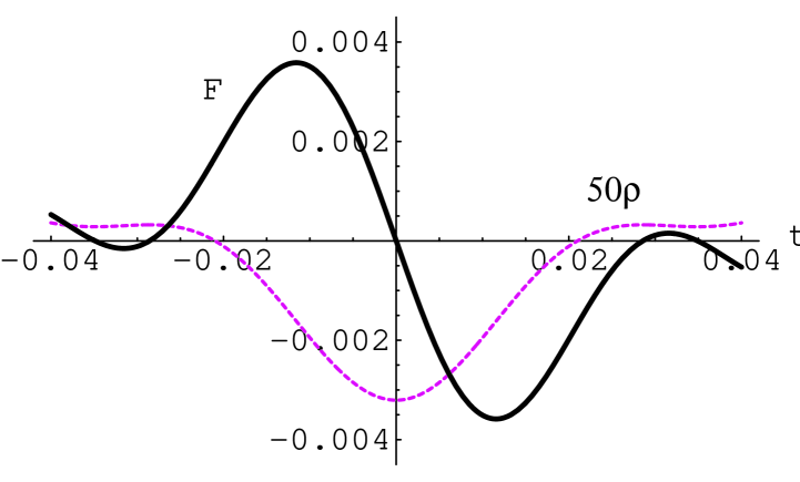
Figure 3: The energy density, $\rho$, and flux, $F$, at $r=2$ are plotted as functions of time. Here we have chosen $p_{0}=1$, $q=10$, and $\Lambda=100$. In order to be visible on this graph, the energy density has been multiplied by a factor of $50$. Our plot is over a timescale small compared to $1/p_{0}=1$, hence we can ignore the long-timescale dependence of $F$ and $\rho$. Note that the sign of the flux changes when the energy density reaches its maximum negative value.

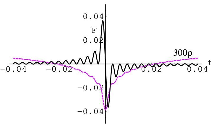
Figure 4: The energy density and flux at $r=2$ are plotted as functions of time, with $p_{0}=1$, $q=10$, and $\Lambda=1000$. In this graph the energy density is multiplied by a factor of $300$ in order to be easily visible. Our plot is over the same timescale as in Fig. 3. The increase in $\Lambda$ results in a higher frequency of oscillation for the flux, $F$. This in turn results in the very short timescale fluctuations of the energy density seen in the figure.

In Fig. 3, as we proceed from negative to positive values of $t$, we see that the energy density starts out approximately constant and positive. It then dips and eventually becomes negative, and afterwards becomes positive and constant again at large $t$. Note that the dip in the energy density is accompanied by a large positive outward flux away from $r=2$, or equivalently a large negative inward flux towards $r=2$. The flux goes through zero when the energy density reaches its minimum value at $t=0$. It then becomes a large and negative outward flux, or equivalently a large and positive inward flux towards $r=2$ as the energy density rises and becomes positive again. Figure 4 shows the more rapid oscillations of the flux when $\Lambda$ is increased. Note that in this case, the energy density undergoes small oscillations superposed upon its approach to a large negative value at $t=0$. As originally discussed in FHR, the energy density may be made arbitrarily negative over an arbitrarily large region at one instant of time. We see here that the accompanying rapidly oscillating fluxes will ensure that the quantum inequalities are not violated, by quickly “pumping” enough positive energy into the region such that the time integral of the energy density over any observer’s worldline will always be positive.

Recall that the spatial region over which the negative energy density appears can be arbitrarily large. In particular, the light travel time over this region can be large compared to the time scale on which the energy density changes sign. One can see this in our plots by comparing Fig. 1 with Fig. 4. The time scale for the variation of the energy density is about two orders of magnitude smaller that the size of the negative energy region. Thus one cannot think of the flow of positive energy into the region as beginning at the boundary and moving inward in a causal way. Rather, the energy density and flux are correlated over spacelike intervals. The energy fluxes depicted in Figs. 3 and 4 are coherent over the entire region. A related example of spacelike correlations in quantum states with negative energy density was discussed in Ref. BFR02 .

III Energy-Flux Correlations in the Vacuum

In this section we discuss a different but related issue - the energy density-flux correlations in the Minkowski vacuum state. We saw in the previous section that, in the Helfer state, the regions of negative energy on a $t=$constant surface were correlated with a rapidly time-varying energy flux. Indeed it is this correlation which ensures that the worldline quantum inequalities are satisfied. As the energy density in a spatial region became negative, there was an accompanying positive energy outflow from (or equivalently, a negative energy inflow into) the region. When the energy density in the region began to rise and become positive again, this was correlated with a positive energy inflow to (or equivalently, a negative energy outflow from) the region.

Does this behavior represent the general case? One might think that the answer is no. The emission of spatially and temporally separated pulses of negative and positive energy by moving mirrors would not appear to fit this profile FD76 ; FD77 ; FR-QIC . However, the moving mirror example is two-dimensional. It has been argued elsewhere that, in four-dimensions, the emission of two separated plane sheets of negative and positive energy would violate the quantum inequalities, unless the positive sheet were infinite in extent BFR02 . So the spatial isolation of negative and positive energy in the moving mirror case may well be an artifact of two-dimensions sphere comment .

So far all of the scenarios we have discussed involved expectation values of the energy density and flux. In this section, we analyze energy density-flux correlation functions in the Minkowski vacuum state, in both two and four dimensions. We find an analogous correlation between energy density and flux here as well. That is, if an energy density fluctuation in a region of the vacuum is initially negative, it is likely to be followed by a flux fluctuation of positive energy into the region. The fact that we see this behavior in the vacuum state as well suggests that it may represent the generic case. The correlations already seem to be “coded” in the vacuum state.

III.1 Two Dimensions

We begin with the calculation of the energy density-flux correlation function for a massless scalar field in the Minkowski vacuum state in two dimensions. The relevant components of the stress-tensor are

$$T^{xt}=-T_{xt}=-\phi,_{x}\phi,_{t}\,,$$ (45)

and

$$T_{tt}=T^{tt}=\frac{1}{2}[{(\phi,_{t})}^{2}+{(\phi,_{x})}^{2}]\,.$$ (46)

Renormalized operators, such as $:{(\phi,_{t})}^{2}:$, can be written as

$$:{(\phi,_{t})}^{2}:={(\phi,_{t})}^{2}-{\langle{(\phi,_{t})}^{2}\rangle}_{0}\,$$ (47)

where ${\langle\rangle}_{0}$ denotes the vacuum expectation value (VEV).

First use Wick’s theorem to write the operator $\phi,_{x}\phi,_{t}:{(\phi,_{t^{\prime}})}^{2}:$ as a sum of normal-ordered products and VEVs:

$$\phi,_{x}\phi,_{t}:{(\phi,_{t^{\prime}})}^{2}: = :\phi,_{x}\phi,_{t}{(\phi,_{t^{\prime}})}^{2}:+2:\phi,_{t}\phi,_{t^{\prime}}:{\langle\phi,_{x}\phi,_{t^{\prime}}\rangle}_{0}$$ (48)

$$+ 2:\phi,_{x}\phi,_{t^{\prime}}:{\langle\phi,_{t}\phi,_{t^{\prime}}\rangle}_{0}+2{\langle\phi,_{x}\phi,_{t^{\prime}}\rangle}_{0}{\langle\phi,_{t}\phi,_{t^{\prime}}\rangle}_{0}\,,$$

where we have also used the fact that $\phi,_{x}\phi,_{t}=:\phi,_{x}\phi,_{t}:$. We can get $\phi,_{x}\phi,_{t}:{(\phi,_{x^{\prime}})}^{2}:$ by letting $t^{\prime}\rightarrow x^{\prime}$.

The flux-energy density correlation function in an arbitrary state is given by

$$C = \langle:T^{xt}(x)::T^{t^{\prime}t^{\prime}}(x^{\prime}):\rangle=\langle T^{xt}(x):T^{t^{\prime}t^{\prime}}(x^{\prime}):\rangle$$ (49)

$$= -\frac{1}{2}\Biggl{[}\langle\phi,_{x}\phi,_{t}:{(\phi,_{t^{\prime}})}^{2}:\rangle+\phi,_{x}\phi,_{t}:{(\phi,_{x^{\prime}})}^{2}:\rangle\Biggr{]}$$

$$= -\frac{1}{2}\Biggl{[}\langle:\phi,_{x}\phi,_{t}{(\phi,_{t^{\prime}})}^{2}:\rangle+\langle:\phi,_{x}\phi,_{t}{(\phi,_{x^{\prime}})}^{2}:\rangle$$

$$+ 2\langle:\phi,_{t}\phi,_{t^{\prime}}:\rangle{\langle\phi,_{x}\phi,_{t^{\prime}}\rangle}_{0}+2\langle:\phi,_{t}\phi,_{x^{\prime}}:\rangle{\langle\phi,_{x}\phi,_{x^{\prime}}\rangle}_{0}$$

$$+ 2\langle:\phi,_{x}\phi,_{t^{\prime}}:\rangle{\langle\phi,_{t}\phi,_{t^{\prime}}\rangle}_{0}+2\langle:\phi,_{x}\phi,_{x^{\prime}}:\rangle{\langle\phi,_{t}\phi,_{x^{\prime}}\rangle}_{0}$$

$$+ 2{\langle\phi,_{x}\phi,_{t^{\prime}}\rangle}_{0}{\langle\phi,_{t}\phi,_{t^{\prime}}\rangle}_{0}+2{\langle\phi,_{x}\phi,_{x^{\prime}}\rangle}_{0}{\langle\phi,_{t}\phi,_{x^{\prime}}\rangle}_{0}\Biggr{]}\,.$$

Now consider the case where the given state is the vacuum. Then all of the VEVs of normal-ordered products vanish and we have

$${\langle T^{xt}(x):T^{t^{\prime}t^{\prime}}(x^{\prime}):\rangle}_{0}=-\left[{\langle\phi,_{x}\phi,_{t^{\prime}}\rangle}_{0}{\langle\phi,_{t}\phi,_{t^{\prime}}\rangle}_{0}+{\langle\phi,_{x}\phi,_{x^{\prime}}\rangle}_{0}{\langle\phi,_{t}\phi,_{x^{\prime}}\rangle}_{0}\right]\,,$$ (50)

with

$${\langle\phi,_{x}\phi,_{t^{\prime}}\rangle}_{0}=\partial_{x}\partial_{t^{\prime}}G=\partial_{x^{\prime}}\partial_{t}G={\langle\phi,_{t}\phi,_{x^{\prime}}\rangle}_{0}\,,$$ (51)

where $G$ is the vacuum two-point function in two-dimensional Minkowski space. Therefore our correlation function becomes

$${\langle T^{xt}(x):T^{t^{\prime}t^{\prime}}(x^{\prime}):\rangle}_{0}=-{\langle\phi,_{x}\phi,_{t^{\prime}}\rangle}_{0}\left({\langle\phi,_{t}\phi,_{t^{\prime}}\rangle}_{0}+{\langle\phi,_{x}\phi,_{x^{\prime}}\rangle}_{0}\right)\,.$$ (52)

In two-dimensional Minkowski space we have that $G=G(\sigma)=-(4\pi)^{-1}\,{\rm ln}\,\sigma$, where $\sigma=(1/2){(x^{\mu}-x^{\prime\mu})}^{2}=(1/2)[{(x-x^{\prime})}^{2}-{(t-t^{\prime})}^{2}]$, and $\partial_{x}G(\sigma)=(x-x^{\prime})G^{\prime}(\sigma)$, where $G^{\prime}=\partial G/\partial\sigma$. Therefore we have that

$${\langle\phi,_{x}\phi,_{t^{\prime}}\rangle}_{0} = \partial_{x}\partial_{t^{\prime}}G(\sigma)=(x-x^{\prime})(t-t^{\prime})G^{\prime\prime}(\sigma)$$

$${\langle\phi,_{t}\phi,_{t^{\prime}}\rangle}_{0} = \partial_{t^{\prime}}[-(t-t^{\prime})G^{\prime}(\sigma)]=G^{\prime}(\sigma)-{(t-t^{\prime})}^{2}\,G^{\prime\prime}(\sigma)$$

$${\langle\phi,_{x}\phi,_{x^{\prime}}\rangle}_{0} = \partial_{x^{\prime}}[(x-x^{\prime})G^{\prime}(\sigma)]=-G^{\prime}(\sigma)-{(x-x^{\prime})}^{2}\,G^{\prime\prime}(\sigma)\,,$$ (53)

and so

$${\langle\phi,_{t}\phi,_{t^{\prime}}\rangle}_{0}+{\langle\phi,_{x}\phi,_{x^{\prime}}\rangle}_{0}=-[{(x-x^{\prime})}^{2}+{(t-t^{\prime})}^{2}]\,G^{\prime\prime}(\sigma)\,.$$ (54)

The flux-energy density correlation function in the vacuum then becomes

$$C=\langle T^{xt}(x):T^{t^{\prime}t^{\prime}}(x^{\prime}):\rangle=(x-x^{\prime})(t-t^{\prime})[{(x-x^{\prime})}^{2}+{(t-t^{\prime})}^{2}]\,{[G^{\prime\prime}(\sigma)]}^{2}$$ (55)

Let $t=0$ and $x^{\prime}=0$, i.e., we look at the correlation between the flux on the $t=0$ surface and the energy density on the $x^{\prime}=0$ worldline. With these choices, our correlation function becomes

$$C=-xt^{\prime}[x^{2}+{t^{\prime}}^{2}]\,{[G^{\prime\prime}(\sigma)]}^{2}\,.$$ (56)

The sign of $C$ in different regions of the $x,t^{\prime}$ plane are shown in Fig. 5.

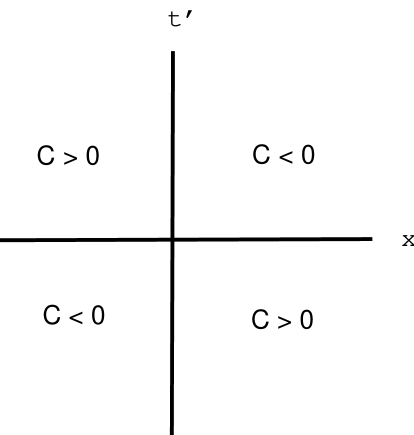
Figure 5: The sign of $C$ in two dimensions is shown in different regions of the $x,t^{\prime}$ plane.

The correlation of the signs of the energy density, $\rho$, and flux, $F=T^{xt}$, is shown in different regions of the $x,t^{\prime}$ plane in Fig. 6.

Case A. For $t^{\prime}<0$ and $x>0$, then $C>0$ and for $t^{\prime}<0$ and $x<0$, then $C<0$. Therefore in Fig. 6(a), we see that if $\rho>0$ initially, then $F(x<0)<0$ and $F(x>0)>0$ subsequently, on average. In Fig. 6(b), if $\rho<0$ initially, then $F(x<0)>0$ and $F(x>0)<0$ subsequently, on average.

Case B. For $t^{\prime}>0$ and $x>0$, then $C<0$ and for $t^{\prime}>0$ and $x<0$, then $C>0$. Therefore in Fig. 6(c), we see that if $F(x<0)>0$ and $F(x>0)<0$ initially, then $\rho>0$ subsequently, on average. In Fig. 6(d), if $F(x<0)<0$ and $F(x>0)>0$ initially, then $\rho<0$ subsequently, on average. Thus in all cases, the sign of the energy density at $x^{\prime}=0$ and the fluxes at $t=0$ are correlated as we would expect.

Figure 6: The correlation of the signs of the energy density and flux in two dimensions is shown in different regions of the $x,t^{\prime}$ plane.

III.2 Four Dimensions

We now compute the vacuum energy density-flux correlation function in four-dimensional Minkowski space. The radial flux is given by

$$F=T^{rt}=\phi^{,r}\phi^{,t}=-T_{rt}=-\phi,_{r}\phi,_{t}\,,$$ (57)

and the energy density by

$$\rho=T^{tt}=\frac{1}{2}(\phi,_{t}\phi,_{t}+\phi,_{i}\phi^{,i})\,.$$ (58)

For the correlation function we have

$$C=\langle:T^{rt}(x)::T^{t^{\prime}t^{\prime}}(x^{\prime}):\rangle=\langle T^{rt}(x):T^{t^{\prime}t^{\prime}}(x^{\prime}):\rangle\,.$$ (59)

A calculation analogous to the one given for two dimensions yields

$$C = -\frac{1}{2}{\langle:\phi,_{r}\phi,_{t}::(\phi,_{t}\phi,_{t}+\phi,_{i}\phi^{,i}):\rangle}_{0}$$ (60)

$$= -{\langle\phi,_{r}\phi,_{t^{\prime}}\rangle}_{0}{\langle\phi,_{t}\phi,_{t^{\prime}}\rangle}_{0}-{\langle\phi,_{r}\phi,_{i^{\prime}}\rangle}_{0}{\langle\phi,_{t}\phi^{,i^{\prime}})\rangle}_{0}\,.$$

Here the vacuum two-point function is $\langle\phi(x)\phi(x^{\prime})\rangle=G(\sigma)=1/(8\pi^{2}\sigma)$, where $\sigma=(1/2)[-{\Delta t}^{2}+{|\Delta{\bf x}|}^{2}]$, and $\Delta t=t-t^{\prime}$, $\Delta{\bf x}={\bf x}-{\bf x^{\prime}}$. So we have that

$${\langle\phi,_{t}\phi,_{t^{\prime}}\rangle}_{0}=\partial_{t}\partial_{t^{\prime}}G(\sigma)=\sigma,_{tt^{\prime}}G^{\prime}(\sigma)+G^{\prime\prime}(\sigma)\sigma,_{t}\sigma,_{t^{\prime}}\,=G^{\prime}(\sigma)-{(\Delta t)}^{2}\,G^{\prime\prime}(\sigma)\,,$$ (61)

and

$${\langle\phi,_{r}\phi,_{t^{\prime}}\rangle}_{0}=\partial_{r}\partial_{t^{\prime}}G(\sigma)=\sigma,_{rt^{\prime}}G^{\prime}(\sigma)+G^{\prime\prime}(\sigma)\sigma,_{r}\sigma,_{t^{\prime}}\,=\Delta t\,\sigma,_{r}\,G^{\prime\prime}(\sigma)\,.$$ (62)

Furthermore,

$${\langle\phi,_{t}\phi^{,i^{\prime}}\rangle}_{0} = -\Delta t\,\sigma^{,i^{\prime}}\,G^{\prime\prime}(\sigma)\,,$$

$${\langle\phi,_{r}\phi,_{i^{\prime}}\rangle}_{0} = \sigma,_{i^{\prime}r}\,G^{\prime}(\sigma)+\sigma,_{i^{\prime}}\sigma,_{r}\,G^{\prime\prime}(\sigma)\,,$$ (63)

so

$${\langle\phi,_{r}\phi,_{i^{\prime}}\rangle}_{0}{\langle\phi,_{t}\phi^{,i^{\prime}}\rangle}_{0}=-\Delta t\,G^{\prime\prime}(\sigma)\,\left[(\sigma^{,i^{\prime}}\,\sigma,_{i^{\prime}r})\,G^{\prime}(\sigma)+(\sigma^{,i^{\prime}}\,\sigma,_{i^{\prime}})\,\sigma,_{r}\,G^{\prime\prime}(\sigma)\,.\right]$$ (64)

We need to calculate the derivatives of $\sigma$ which appear in the above expression. The scalar quantity $\sigma^{,i^{\prime}}\,\sigma,_{i^{\prime}}$ is most easily computed in Cartesian coordinates, where $\sigma,_{i^{\prime}}=-\Delta x^{i}$ and hence $\sigma^{,i^{\prime}}\,\sigma,_{i^{\prime}}=|\Delta{\bf x}|^{2}$. We consider the case when ${\bf x^{\prime}}=0$. We then find

$$\sigma^{,i^{\prime}}\sigma,_{i^{\prime}r} = r$$

$$\sigma,_{r} = r$$

$$\sigma^{,i^{\prime}}\sigma,_{i^{\prime}} = r^{2}\,.$$ (65)

As a result our energy density-flux vacuum correlation function reduces to

$$C=r\,{\Delta t}\left[{({\Delta t})}^{2}+r^{2}\right]\,{[G^{\prime\prime}(\sigma)]}^{2}\,,$$ (66)

where $\sigma=(1/2)[r^{2}-{({\Delta t})}^{2}]$ for $r^{\prime}=0$. Note that the sign of $C$ depends only on the sign of $\Delta t$. Recall that ${\Delta t}=t-t^{\prime}$. If $t>t^{\prime}$, then $C>0$. Consequently, $\rho(t^{\prime})>0$ implies $F=T^{rt}(t)>0$ on average, as illustrated in Fig. 7, and $\rho(t^{\prime})<0$ implies $F=T^{rt}(t)<0$ on average. This is consistent with our two-dimensional results. If $\rho>0$ at the origin at one time, the flux at a later time is likely to be outgoing. Similarly, if $\rho<0$ at one time, the later flux is more likely to be ingoing. We can also reverse the time order. An outgoing flux at $t$ is correlated with $\rho<0$ at $t^{\prime}>t$, and an ingoing flux at $t$ is correlated with $\rho>0$ at $t^{\prime}>t$.

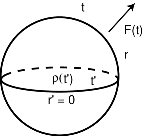
Figure 7: Here the relation between the energy density at time $t^{\prime}$ and $r^{\prime}=0$ and the flux $F$ at time $t$ and radius $r$ is sketched. A positive energy density at an earlier time $t^{\prime}$ is correlated with an outgoing flux at a later time $t$, and vice versa.

Lastly we discuss the falloff of the correlations in both two and four dimensions. In two dimensions, choosing $t=0$, we have ${\Delta t}=t-t^{\prime}=-t^{\prime}$ and so

$$C=-xt^{\prime}\,(x^{2}+{t^{\prime}}^{2})\,{[G^{\prime\prime}(\sigma)]}^{2}\,.$$ (67)

Since in two dimensions $G=-(4\pi)^{-1}\,{\rm ln}\,\sigma$, $G^{\prime\prime}=1/(4\pi\sigma^{2})\propto-1/{(x^{2}-{t^{\prime}}^{2})}^{2}$. If we let $x\rightarrow\infty$, with $t^{\prime}$ fixed, then

$$C\sim-\frac{t^{\prime}}{x^{5}}\,.$$ (68)

Alternatively, if we let $t^{\prime}\rightarrow\infty$, with $x$ fixed, then

$$C\sim-\frac{x}{{(t^{\prime})}^{5}}\,.$$ (69)

Thus the falloff is symmetrical for both spacelike and timelike separations.

In four dimensions, with $r^{\prime}=0$ and since $G=1/(8\pi^{2}\sigma)$, $G^{\prime\prime}=1/(4\pi^{2}\sigma^{3})\propto 1/{[r^{2}-{({\Delta t})}^{2}]}^{3}$, we have that for $r\rightarrow\infty$, with $\Delta t$ fixed, then

$$C\sim\frac{\Delta t}{r^{9}}\,.$$ (70)

For ${\Delta t}\rightarrow\infty$, with $r$ fixed,

$$C\sim\frac{r}{{(\Delta t)}^{9}}\,.$$ (71)

and again the falloff is symmetric between space and time. Note also that $C$ has the same form in two and four dimensions, apart from the difference in the expression for $G(\sigma)$.

IV Conclusions

In this paper we have examined in detail the behavior and correlation of energy density and flux in a “Helfer state”. This state, first suggested by Adam Helfer, is one in which the energy density can be made arbitrarily large and negative over an arbitrarily large region of space, even in Minkowski spacetime. However, this can be achieved only at one instant in time. For the quantum inequalities to hold, there must be large time-varying fluxes associated with these states. We show that this is in fact the case, and analyze the correlated behavior of the expectation values of the flux and energy density, in order to gain a deeper insight into these remarkable quantum states.

In the second part of the paper, we examine the energy density-flux correlation function in the Minkowski vacuum state. Although we now work with correlation functions, as opposed to expectation values, we find qualitatively similar behavior for energy density and flux fluctuations. An initial negative energy vacuum fluctuation in some region of space is correlated with a subsequent flux fluctuation of positive energy into the region.

The quantum inequalities place a (negative) lower bound on the distribution function for energy density vacuum fluctuations Chris_comment . Perhaps the mechanism which ensures that the quantum inequalities hold in the Helfer state, as well as in other quantum states associated with negative energy, is, at least in some sense, already “encoded” in the fluctuations of the vacuum.

- (1) H. Epstein, V. Glaser, and A. Jaffe, Nuovo Cim. 36, 1016 (1965).
- (2) S.W. Hawking, Comm. in Math. Phys. 43, 199 (1975).
- (3) P.C.W. Davies, S.A. Fulling, and W.G. Unruh, Phys. Rev. D13, 2720 (1976); P. Candelas, Phys. Rev. D21, 2185 (1980).
- (4) R.E. Slusher, L.W. Hollberg, B. Yurke, J.C. Mertz, and J. F. Valley, Phys. Rev. Lett. 55, 2409, (1985).
- (5) H.B.G. Casimir, Proc. K. Ned. Akad. Wet. 51, 793 (1948); L.S. Brown and G.J. Maclay, Phys. Rev. 184, 1272 (1969).
- (6) L.H. Ford, Proc. Roy. Soc. Lond. A364, 227 (1978).
- (7) L.H. Ford, Phys. Rev. D43, 3972 (1991).
- (8) M. Morris and K. Thorne, Am. J. Phys. 56, 395 (1988).
- (9) M. Morris, K. Thorne, and U. Yurtsever, Phys. Rev. Lett. 61, 1446 (1988).
- (10) M. Alcubierre, Class. Quantum Grav. 11, L73 (1994).
- (11) M.J. Pfenning and L.H. Ford, Class. Quantum Grav. 14, 1743 (1997), gr-qc/9702026.
- (12) A.E. Everett and T.A. Roman, Phys. Rev. D56, 2100 (1997), gr-qc/9702026.
- (13) S.V. Krasnikov, Phys. Rev. D57, 4760 (1998), gr-qc/9511068.
- (14) S.W. Hawking, Phys. Rev. D46, 603 (1992).
- (15) T.A. Roman, Proceedings of the Tenth Marcel Grossmann Meeting on General Relativity, edited by M. Novello, S. Perez Bergliaffa and R. Ruffini (World Scientific, Singapore, 2005), part C, p. 1909.
- (16) C.J. Fewster, Energy inequalities in quantum field theory, in XIVth International Congress on Mathematical Physics, edited by J.C. Zambrini (World Scientific, Singapore, 2005). Expanded and updated version: math-ph/0501073.
- (17) L.H. Ford, ”Spacetime in Semiclassical Gravity”, in 100 Years of Relativity - Space-time Structure: Einstein and Beyond, edited by A. Ashtekar, (World Scientific, Singapore, 2006), gr-qc/0504096.
- (18) A.D. Helfer, Class. Quantum Grav. 13, L129 (1996), gr-qc/9602060.
- (19) L.H. Ford, A.D. Helfer, and T.A. Roman, Phys. Rev. D66, 124012 (2002).
- (20) See J.D. Jackson, Classical Electrodynamics, 2nd Edition, John Wiley & Sons, Inc., New York (1975), p. 101, Fig. 3.7 and discussion after Eq. (3.62).
- (21) A. Borde, L.H. Ford, and T.A. Roman, Phys. Rev. D65, 084002 (2002), gr-qc/0109061.
- (22) S.A. Fulling and P.C.W. Davies, Proc. R. Soc. London A348, 393 (1976).
- (23) P.C.W. Davies and S.A. Fulling, ibid, A356, 237 (1977).
- (24) L.H. Ford and T.A. Roman, Phys. Rev. D60, 104018 (1999), gr-qc/9901074.
- (25) A more appropriate analog in four-dimensions might be two concentric shells of positive and negative energy as discussed in Ref. BFR02 .
- (26) This insight is due to Chris Fewster (unpublished).