Chemical evolution of the Small Magellanic Cloud based on planetary nebulae

Abstract

Aims. We investigate the chemical evolution of the Small Magellanic Cloud (SMC) based on abundance data of planetary nebulae (PNe). The main goal is to investigate the time evolution of the oxygen abundance in this galaxy by deriving an age-metallicity relation. Such a relation is of fundamental importance as an observational constraint of chemical evolution models of the SMC.

Methods. We have used high quality PNe data in order to derive the properties of the progenitor stars, so that the stellar ages could be estimated. We collected a large number of measured spectral fluxes for each nebula, and derived accurate physical parameters and nebular abundances. New spectral data for a sample of SMC PNe obtained between 1999 and 2002 are also presented. These data are used together with data available in the literature to improve the accuracy of the fluxes for each spectral line.

Results. We obtained accurate chemical abundances for PNe in the Small Magellanic Cloud, which can be useful as tools in the study of the chemical evolution of this galaxy and of Local Group galaxies. We present the resulting oxygen versus age diagram and a similar relation involving the [Fe/H] metallicity based on a correlation with stellar data. We discuss the implications of the derived age-metallicity relation for the SMC formation, in particular by suggesting a star formation burst in the last 2–3 Gyr.

1 Introduction

A comprehensive study of the chemical enrichment in a given stellar system involves the determination of accurate abundances and the building of several chemical diagrams showing the evolution of the abundances of different elements and their variation with time. In particular, diagrams of the abundances as a function of age are fundamental in order to decrease the number of possible solutions of chemical evolution models, working as a strong constraint to these models. The understanding of the evolutionary process of the Magellanic Clouds, and of the Small Magellanic Cloud (SMC) in particular, is important in many aspects: the metallicity of the SMC is closer to that of a primordial galaxy than the Large Magellanic Cloud (LMC) or the Galaxy, its distance is well known and the local reddening is considerably lower than that of the Galactic disk.

The star formation histories of the LMC and SMC seem to present different patterns from each other, and are in many respects still controversial (cf. Olszewski et al. olszewski (1996)). Bertelli et al. (bertelli (1992)) pointed out that the LMC experienced an episode of star formation around 3-5 Gyr ago, while the star formation history of the SMC would indicate a constant formation rate during the last 2-12 Gyr (Dolphin et al. dolphin (2001)). On the other hand, Piatti et al. (piatti2 (2005)) studied a sample of clusters in the SMC and concluded that there is a peak in their age distribution at 2.5 Gyr, which corresponds to a very close encounter between the LMC and the SMC according to dynamical models, in agreement with the results from the bursting model by Pagel and Tautvaišiene (pagel (1998)), adopting a burst that occurred 3 Gyr ago. More recent work on the SMC, especially on the basis of the age distribution of stellar clusters, is consistent with a star formation burst in the last few Gyr, as we will discuss in more detail in Section 6.

In this work, we obtain accurate chemical abundances for planetary nebulae in the SMC and use these results to study the chemical evolution of this galaxy. To do this, high quality PNe data are needed, especially to derive the properties of PNe progenitors to estimate their ages. Our first goal was to collect a large number of measured spectral fluxes for each SMC PNe, in order to derive accurate physical parameters and abundances. We also present new spectral data for a sample of SMC PNe obtained by our group between 1999 and 2002. These data are combined with data available in the literature to improve the accuracy of the fluxes for each PNe spectral line. Finally, we present an age-metallicity relationship in the form of oxygen abundances relative to the sun as a function of age and [Fe/H]–age diagrams, and discuss their implications for SMC formation.

2 The sample

2.1 Observations and data reduction

Observations were performed using telescopes at ESO La Silla (1.52 m) and at the Laboratório Nacional de Astrofísica (LNA), Brazil (1.60 m). Weather conditions are normally different in both observatories: at ESO/La Silla the average seeing is typically smaller than 1”, and for measurements at this site we used slit width of 1”. On the other hand, at LNA we adopted 1.5” slit width due to the poorer seeing conditions. All measurements were performed with airmass smaller than $X$ =1.5 in order to keep the spectrophotometric accuracy of the results. In both observatories, long east-west slits were used in all cases. Also, in both observatories, Boller & Chivens Cassegrain spectrographs were used; at ESO with CCD and grating allowing a reciprocal dispersion of about 2.5 Å/pixel, and at LNA with a CCD and grating with smaller dispersion, namely, 4.4 Å/pixel. This sample includes 36 objects, and the log of the observations is given in Table 1. In this table we also included the exposures times $t_{ex}$ in seconds and the extinction coefficient $c_{ext}$ derived from the H$\alpha$/H$\beta$ ratios assuming Case B (Osterbrock osterbrock (1989)) and adopting the extinction law by Cardelli et al. (cardelli (1989)). The PNe marked with an asterisk have been included in Costa et al. (costa (2000)), but for 8 of these objects new observations have been made.

Table 1: Log of the observations.

Object	Date	Site	$t_{ex}(s)$	$c_{ext}$	Object	Date	Site	$t_{ex}(s)$	$c_{ext}$
SMP 1*	1999 Aug 19	ESO	3600	0.18	SMP 16*	1999 Dec 29	ESO	2400	0.03
	2002 Set 25	ESO	3600	0.23	SMP 17*	1999 Aug 17	ESO	1800	0.64
SMP 2*	1999 Aug 19	ESO	2400	0.18	SMP 18*	1999 Aug 17	ESO	2400	0.28
SMP 3*	1999 Aug 19	ESO	2100	0.07		2002 Oct 11	ESO	3600	0.37
SMP 4*	1999 Aug 20	ESO	2400	0.00	SMP 19*	1999 Aug 18	ESO	3600	0.45
	2002 Oct 12	ESO	3000	0,00	SMP 20	2002 Oct 11	ESO	2400	0.00
SMP 5*	1999 Jul 18	LNA	2400	0.67	SMP 21*	1999 Dec 28	ESO	2400	0.26
SMP 6*	1999 Jul 18	LNA	2400	0.42	SMP 22*	1999 Aug 17	ESO	1800	0.39
	2002 Set 25	ESO	5400	0.45	SMP 23*	1999 Aug 20	ESO	2400	0.00
	2002 Oct 13	ESO	2400	0.61	SMP 24	2002 Oct 10	ESO	3000	0.03
SMP 7*	1999 Aug 15	ESO	3600	0.15	SMP 25*	1999 Dec 28	ESO	3000	0.00
SMP 8*	1999 Aug 20	ESO	2400	0.03	SMP 26	2002 Set 27	ESO	3600	0.00
	2002 Set 27	ESO	2400	0.55	SMP 27	2002 Set 27	ESO	2400	0.00
SMP 9*	1999 Jul 20	LNA	2400	0.95	SMP 28	2002 Oct 10	ESO	3600	0.00
	1999 Dec 28	ESO	3000	0.92	MGPN 1	2002 Oct 09	ESO	3600	2.38
SMP 10*	1999 Jul 20	LNA	2400	0.90	MGPN 2	2002 Oct 10	ESO	3600	2.87
	2002 Set 28	ESO	3600	0.07	MGPN 3	2002 Oct 11	ESO	3600	0.16
SMP 11*	1999 Dec 26	ESO	2400	0.59	MGPN 5	2002 Oct 12	ESO	3600	0.00
	2002 Oct 08	ESO	3600	0.62	MGPN 7	2002 Oct 13	ESO	3600	0.99
SMP 12*	1999 Aug 16	ESO	3600	0.00	MGPN 11	2002 Oct 09	ESO	3600	1.72
SMP 13*	1999 Dec 26	ESO	2400	0.05	MGPN 13	2002 Set 27	ESO	2400	0.39
	2002 Set 28	ESO	3600	0.64	[M95] 9*	1999 Aug 15	ESO	3600	0.24
SMP 14*	1999 Dec 27	ESO	2400	0.05
SMP 15	1999 Aug 16	ESO	3600	0.26
	2002 Oct 10	ESO	3000	0.00

Image reduction and analysis were performed using the IRAF package, including the classical procedure to reduce long slit spectra: bias, dark and flat-field corrections, spectral profile extraction, wavelength and flux calibrations. Atmospheric extinction was corrected using mean coefficients for each observatory, and flux calibration was secured by the observation of standard stars (at least three) every night. Emission line fluxes were calculated assuming Gaussian profiles, and a Gaussian de-blending routine was used when necessary. Fig. 1 presents a sample spectrum for the planetary nebula SMP 15 in the SMC, taken in October, 2002.

Figure 1: An example of a spectrum of the planetary nebula SMP 15 in the SMC.

The PNe sample given in Table 1 was observed in order to improve the measured line fluxes. In Table 2 (available in electronic form at the CDS), we report the new measured fluxes with errors including those from Costa et al. (costa (2000)) for the lines used in this work. These fluxes were corrected from reddening and are presented in the H$\beta$ = 100 scale. Typical errors at the end of the spectrophotometric calibration process depend mainly on the derived sensitivity function for each night, which is related to distinct factors like the S/N for each line, the adopted atmospheric extinction coefficient and photometric quality of the night. Uncertainties in the individual measurements of each line are estimated as about 4% for lines stronger than 100 (in the H$\beta$=100 scale), 10% for lines between 10 and 100, 15% for lines between 1 and 10, and 32% for lines weaker than 1 in the same scale. The errors quoted in Table 2 are the resulting dispersions from the average on the individual measurements. In this table, the first column gives the wavelength (in Å) and the ion responsible for the transition, while the remaining columns give the measured fluxes in the H$\beta$ = 100 scale, followed by the estimated uncertainty and the number of measurements taken. In this table, as in all remaining tables of this paper, no errors are given when only one measurement was available.

2.2 Additional objects

In order to obtain a more significant sample, we have also taken into account some SMC nebulae from the literature, as well as flux measurements of the nebulae given in Table 1 by different sources. The new objects are SMP 32, SMP 34, MGPN 6, MGPN8, MGPN 9, MGPN 10, MGPN 12, Ma01, Ma02, and [M95] 8. The total sample includes then 46 objects, and is shown in Table 3. In this table, which is also available at the CDS, the final flux data used to derive the physical parameters of the nebulae are presented in the same form as in Table 2. The line fluxes given in this table are simple averages of our data and other data compiled from the literature, taken from Webster (webster (1976)), Osmer (osmer (1976)), Dufour & Killen (dufour (1977)), Aller et al. (aller (1981)), Monk et al. (monk (1988)), Boroson & Liebert (boronson (1989)), Meatheringham & Dopita (1991a , 1991b ), Vassiliadis et al. (vassiliadis (1992)), Meyssonnier (meyssonier (1995)), and Leisy & Dennefeld (leisy1 (1996)). Too discrepant flux values were discarded.

The CIII] $\lambda$1907,1909 fluxes as given in Table 3 were measured from IUE spectra, adopting an average extinction coefficient. This coefficient was taken as a simple, unweighted average from several references, and is given in Table 4, where the original references are shown. These references include Monk et al. (monk (1988)), Boroson & Liebert (boronson (1989)), Meatheringham et al. (1991a , 1991b ), Vassiliadis et al. (vassiliadis (1992)), Meyssonier (meyssonier (1995)), Costa et al. (costa (2000)), Stanghellini et al. (stanghellini (2003)), Leisy (leisy2 (2006)), and Leisy & Dennefeld (leisy3 (2006)), apart from our own measurements.

Table 4: Average extinction coefficients and references.

Object	$\langle c_{ext}\rangle$	References∗	Object	$\langle c_{ext}\rangle$	References∗
SMP 1	$0.26\pm 0.07$	3,1,2,8,9	SMP 24	$0.03\pm 0.03$	1,2,9
SMP 2	$0.28\pm 0.09$	3,2,6,8	SMP 25	$0.19\pm 0.19$	1,2,6,9
SMP 3	$0.06\pm 0.10$	3,2,6,8	SMP 26	$0.31\pm 0.24$	1,2,6,9
SMP 4	$0.17\pm 0.25$	3,1,2	SMP 27	$0.03\pm 0.04$	3,2,6,8,9
SMP 5	$0.43\pm 0.28$	3,6,8	SMP 28	$0.15\pm 0.09$	3,2,6,8
SMP 6	$0.57\pm 0.15$	3,1,2,6,8,9	SMP 32	0.00	2
SMP 7	$0.15\pm 0.09$	3,4,2,6	SMP 34	$0.10\pm 0.09$	2,9
SMP 8	$0.27\pm 0.25$	3,1,2,8,9	MGPN 1	2.38	1
SMP 9	$0.93\pm 0.02$	3,1	MGPN 2	2.87	1
SMP 10	$0.52\pm 0.42$	1,2,8	MGPN 3	0.16	1
SMP 11	$0.56\pm 0.26$	3,1,7,2,6,8,9	MGPN 5	0.00	1
SMP 12	$0.14\pm 0.19$	3,2,9	MGPN 6	0.26	5
SMP 13	$0.30\pm 0.21$	3,1,2,6,8,9	MGPN 7	$0.99\pm 0.01$	1,2
SMP 14	$0.16\pm 0.11$	3,2,6,8,9	MGPN 8	0.00	5
SMP 15	$0.16\pm 0.12$	3,1,2	MGPN 9	1.08	2
SMP 16	$0.02\pm 0.02$	3,2	MGPN 10	0.12	5
SMP 17	$0.65\pm 0.24$	3,2,8	MGPN 11	1.72	1
SMP 18	$0.32\pm 0.16$	3,1,8,9	MGPN 12	0.56	2
SMP 19	$0.37\pm 0.23$	3,2,8,9	MGPN 13	$0.34\pm 0.08$	1,2
SMP 20	$0.03\pm 0.03$	1,2,6	Ma 01	0.00	5
SMP 21	$0.24\pm 0.18$	3,1,6	Ma 02	0.99	5
SMP 22	$0.29\pm 0.14$	3,2,6,9	[M95] 8	0.63	8
SMP 23	$0.05\pm 0.06$	3,2,6,9	[M95] 9	0.24	3

• References of individual coefficients

• (1) This work

• (2) Leisy (leisy2 (2006)), Leisy & Dennefeld (leisy3 (2006))

• (3) Costa et al. (costa (2000))

• (4) Meyssonnier (meyssonier (1995))

• (5) Vassiliadis et al. (vassiliadis (1992))

• (6) Meatheringham & Dopita (1991a , 1991b )

• (7) Boronson & Liebert (boronson (1989))

• (8) Monk et al. (monk (1988))

• (9) Stanghellini et al. (stanghellini (2003))

3 Physical parameters

Mean electron densities $N_{e}$ were estimated from the [SII] line ratio $\lambda$6716/6730. The observational dispersions in [SII] line fluxes were taken into account for $N_{e}$ calculations, giving a range of possible solutions for [SII] line ratios between 0.45 and 1.44. Mean electron temperatures $T_{e}$ were derived from the lines ratios [NII] ($\lambda$6548+6583)/5755 and [OIII] ($\lambda$4959+5007)/4363. Table 5 shows the estimated mean electron densities (cm^-3) and temperatures (K) for each PNe. Errors were estimated by using classical error propagation both for electron densities and temperatures, leading to typical uncertainties of up to a factor of 2 -3 in densities and of 10% to 30% in the temperatures. It should be noted, however, that a proper account for the true accuracy of the derived physical parameters has to consider the number of flux measurements for each line. Those with few measurements may induce artificially low dispersions in their final values. In the case of a single measurement, again no error estimates are given. When the [SII] line ratio was outside the range 0.45–1.44, upper and lower electron density limits of $N_{e}=50000\,$cm^-3 and 10 cm^-3 respectively, were considered. Fig. 2 shows the final estimated $T_{e}$ from [NII] and [OIII] lines. Error bars are plotted only for objects having more than one temperature determination. For those objects with a single measurement, an uncertainty of up to 30% was estimated, as mentioned. For most nebulae there is a general agreement between the temperatures, in the sense that they do not differ by more than about 50%, a result similar to that obtained by Kingsburgh & Barlow (kingsburgh (1994)) for Galactic PNe. However, the ratio of the [NII] to [OIII] temperatures depends on the excitation conditions, and we find that for about 1/3 of the objects in the sample, the temperatures derived from [NII] lines are appreciably higher, which probably reflects the physical conditions in different parts of the nebulae. For the estimate of abundances, we decided to use $T_{e}$ from [OIII] lines due to the larger uncertainties in the [NII] fluxes.

Figure 2: Electron temperatures $T_{e}$ of PNe estimated from [NII] and [OIII] lines. Error bars are provided only for objects having more than one temperature determination.

Table 5: Physical parameters: electron densities and temperatures.

Object	$N_{e}$[SII]	$T_{e}$[NII]	$T_{e}$[OIII]	Object	$N_{e}$[SII]	$T_{e}$[NII]	$T_{e}$[OIII]
SMP 1	$>50000$	$15720\pm 2260$	$11360\pm 1090$	SMP 24	1240	$13940\pm 2760$	$11720\pm 1030$
SMP 2	2740	$12650\pm 2500$	$14040\pm 930$	SMP 25	740	$33510\pm 12820$	$36260\pm 2400$
SMP 3	4910		$12990\pm 610$	SMP 26	840	$13330\pm 680$	$18800\pm 3200$
SMP 4	1470	$50230\pm 32120$	$15040\pm 1050$	SMP 27	11250	$18590\pm 10230$	$12250\pm 3200$
SMP 5	4630	$12600\pm 790$	$13280\pm 860$	SMP 28	2360	$18250\pm 1020$	$23250\pm 2790$
SMP 6	$>50000$	$13960\pm 1550$	$13740\pm 720$	SMP 32	1790		14760
SMP 7	1790	$49860\pm 13260$	$16950\pm 1480$	SMP 34	490	9770	12940
SMP 8	1790	$19070\pm 8380$	$12180\pm 920$	MGPN 1	460	$58890\pm 10570$	$14680\pm 330$
SMP 9	790	$36460\pm 20210$	$13850\pm 620$	MGPN 2	500		$25440\pm 2060$
SMP 10	895	$26610\pm 6620$	$11180\pm 1000$	MGPN 3	580		$17970\pm 330$
SMP 11	1190	$22290\pm 4300$	$15140\pm 1410$	MGPN 5	100		$17700\pm 6020$
SMP 12	580		$13300\pm 760$	MGPN 6	580		85370
SMP 13	1730		$12300\pm 1320$	MGPN 7	445	$23090\pm 650$	$15960\pm 740$
SMP 14	1470		$13450\pm 590$	MGPN 8	$>50000$		23900
SMP 15	3350	$18500\pm 2910$	$12440\pm 840$	MGPN 9	4010	36200	20870
SMP 16	$>50000$	$9180\pm 700$	$11000\pm 1300$	MGPN 10	580		25820
SMP 17	$>50000$	$10810\pm 2950$	$11560\pm 920$	MGPN 11	$<10$	$22290\pm 1100$	$16700\pm 5900$
SMP 18	6020	$17260\pm 7840$	$10740\pm 1900$	MGPN 12	1170	12760	22030
SMP 19	4510	$29150\pm 19590$	$13470\pm 1900$	MGPN 13	2470		$20130\pm 3620$
SMP 20	1470	$38040\pm 2870$	$13000\pm 860$	Ma 01	580		19690
SMP 21	11250	$20740\pm 12060$	$23540\pm 9120$	Ma 02	580		20990
SMP 22	1660	$12530\pm 1080$	$25720\pm 1950$	[M95] 8
SMP 23	580		$13265\pm 319$	[M95] 9	230		$12400\pm 740$

4 Abundances

4.1 Helium abundances

Helium abundances were estimated using the mean electron temperatures and densities derived in the previous section. In view of their relatively intense flux, the lines used to derive the He abundance were HeI $\lambda$5876 and HeII $\lambda$4686. The total helium abundance is then given by

$${{\rm He}\over{\rm H}}={\alpha_{5876}\ X^{2}_{5876}+\alpha_{4676}\ X^{2}_{4676}\over\alpha_{4861}\ X^{2}_{4861}}\,$$ (1)

where $\alpha_{\lambda}$ are the total recombination coefficients and $X_{\lambda}$ represent the fluxes in units of the H$\beta$ line flux. The total recombination coefficients are taken from Péquignot et al. (daniel (1991)). In the case of HeI lines, corrections of important collisional effects were made in the recombination coefficients, using the collision-to-recombination correction factors from Kingdon & Ferland (kingdon (1995)).

Table 6 shows the derived ionic and total helium abundances relative to hydrogen, by number of atoms. In this table and in the next one the notation $2\times 10^{-4}=2(-4)$ has been used. Errors were estimated by propagating the observational uncertainties in HeI and HeII line fluxes and in the $T_{e}$ and $N_{e}$ derivation. In the case of MG7 the He abundance was calculated from the $\lambda$4471 line. For MG8 and MG13 average values have been used.

Table 6: Helium ionic and total abundances.

Object	HeI	HeII	He	Object	HeI	HeII	He
SMP 1	$0.071\pm 0.012$	$1(-3)\pm 2(-4)$	$0.072\pm 0.012$	SMP 24	$0.097\pm 0.011$		$0.097\pm 0.011$
SMP 2	$0.072\pm 0.008$	$0.018\pm 0.003$	$0.090\pm 0.009$	SMP 25	$0.057\pm 0.006$	$4(-3)\pm 9(-4)$	$0.061\pm 0.006$
SMP 3	$0.114\pm 0.001$	$7(-3)\pm 8(-4)$	$0.121\pm 0.001$	SMP 26	$0.058\pm 0.017$	$0.018\pm 0.002$	$0.075\pm 0.017$
SMP 4	$0.124\pm 0.011$	$2(-4)\pm 2(-4)$	$0.125\pm 0.011$	SMP 27	$0.091\pm 0.009$	$1(-3)\pm 3(-5)$	$0.092\pm 0.009$
SMP 5	$0.069\pm 0.009$	$0.026\pm 0.002$	$0.095\pm 0.009$	SMP 28	$0.089\pm 0.009$	$12(-3)\pm 6(-4)$	$0.100\pm 0.009$
SMP 6	$0.087\pm 0.010$	$3(-4)\pm 4(-6)$	$0.088\pm 0.010$	SMP 32	$0.085\pm 0.007$	0.006	$0.091\pm 0.007$
SMP 7	$0.080\pm 0.008$	$4(-3)\pm 7(-4)$	$0.084\pm 0.008$	SMP 34	$0.079\pm 0.008$	0.006	$0.085\pm 0.008$
SMP 8	$0.099\pm 0.014$		$0.099\pm 0.014$	MGPN 1	$0.151\pm 0.023$	$11(-3)\pm 3(-4)$	$0.161\pm 0.023$
SMP 9	$0.030\pm 0.004$	$0.034\pm 0.006$	$0.064\pm 0.007$	MGPN 2	$0.067\pm 0.026$	$2(-3)\pm 1(-4)$	$0.069\pm 0.026$
SMP 10	$0.087\pm 0.011$	$6(-4)\pm 6(-4)$	$0.088\pm 0.011$	MGPN 3	$0.129\pm 0.014$	$7(-3)\pm 2(-4)$	$0.136\pm 0.014$
SMP 11	$0.085\pm 0.010$	$1(-3)\pm 8(-5)$	$0.086\pm 0.010$	MGPN 5	$0.067\pm 0.038$	$0.034\pm 0.002$	$0.101\pm 0.038$
SMP 12	$0.107\pm 0.009$	$1(-3)\pm 3(-4)$	$0.108\pm 0.009$	MGPN 6	$0.149\pm 0.012$	0.002	$0.151\pm 0.012$
SMP 13	$0.107\pm 0.015$	$2(-4)\pm 7(-6)$	$0.107\pm 0.015$	MGPN 7	$0.104\pm 0.050$	$0.013\pm 0.005$	$0.117\pm 0.050$
SMP 14	$0.062\pm 0.007$	$0.021\pm 0.004$	$0.084\pm 0.008$	MGPN 8	$0.019\pm 0.006$	$5(-3)\pm 6(-5)$	$0.024\pm 0.006$
SMP 15	$0.104\pm 0.011$	$5(-4)\pm 3(-4)$	$0.105\pm 0.011$	MGPN 9	$0.063\pm 0.007$	$1(-4)$	$0.063\pm 0.007$
SMP 16	$0.062\pm 0.008$	$6(-4)\pm 3(-4)$	$0.063\pm 0.008$	MGPN 10	$0.070\pm 0.006$	0.019	$0.089\pm 0.006$
SMP 17	$0.103\pm 0.024$	$1(-3)\pm 2(-4)$	$0.104\pm 0.024$	MGPN 11	$0.218\pm 0.036$	$0.008\pm 0.004$	$0.227\pm 0.036$
SMP 18	$0.086\pm 0.008$		$0.086\pm 0.008$	MGPN 12	$0.118\pm 0.010$	0.013	$0.131\pm 0.010$
SMP 19	$0.055\pm 0.008$	$0.026\pm 0.003$	$0.081\pm 0.009$	MGPN 13	$0.006\pm 0.002$	$0.031\pm 0.003$	$0.037\pm 0.003$
SMP 20	$0.118\pm 0.020$	$2(-4)\pm 4(-6)$	$0.119\pm 0.020$	Ma 01	$0.167\pm 0.014$	0.007	$0.174\pm 0.014$
SMP 21	$0.075\pm 0.017$	$0.007\pm 0.001$	$0.082\pm 0.017$	Ma 02	$0.049\pm 0.004$	0.011	$0.061\pm 0.004$
SMP 22	$0.062\pm 0.007$	$11(-3)\pm 9(-4)$	$0.073\pm 0.007$	[M95] 8
SMP 23	$0.095\pm 0.011$	$2(-3)\pm 2(-4)$	$0.097\pm 0.011$	[M95] 9	$0.083\pm 0.007$		$0.083\pm 0.007$

4.2 Ionic and elemental abundances

Ionic abundances were estimated for the ions present in the optical spectra by solving the statistical equilibrium equations for a three-level atom model, including radiative and collisional transitions. The resulting ionic abundances with uncertainties are given in Table 7 (available at the CDS). In this table, the first line of each nebula gives the ionic abundances by number of atoms relative to hydrogen, while the second line gives the uncertainties. The asterisks (*) indicate that the corresponding dispersion is due to different measurements in electronic temperature and/or densities, while double asterisks (**) indicate that the dispersions are due to different measurements in the ionic line only. The sign (:) indicates only one measurement of the electron temperature, density and ionic line, so that no errors are given. The elemental abundances were then derived using ionization correction factors (ICF). We adopted the same ICF given by Escudero et al. (escudero (2004)) to account for unobserved ions of each element. The corresponding elemental abundances are given in columns 2 to 7 of Table 8, in the form $\epsilon({\rm X})=\log({\rm X/H})+12$, as usual. It should be noted that the uncertainties given in Table 8 are formal uncertainties, which are essentially an estimate of the dispersion in the considered measurements, as discussed in Section 2. A more realistic estimate of the errors may be obtained from a comparison with other determinations in the literature (cf. section 4.4), and may reach about 0.1 to 0.2 dex for the best measured elements, and about 0.3 dex for those with the weakest lines.

In order to derive the carbon abundances we adopted the following procedure: ionic abundances of carbon and oxygen were derived from the ultraviolet CIII]$\lambda$1909 and OIII]$\lambda$1663 lines, according to the formulae by Aller (aller2 (1984)). Rola & Stasińska (rola (1994)) pointed out that the elemental ratio C/O can be safely approximated by the C⁺²/O⁺² ratio, except for very low excitation objects (those with [OIII]$\lambda$5007/H$\beta<3$), for which this assumption is not valid. We derived the C/O ratio, and, by taking the oxygen abundance derived from the optical data, the carbon abundances were derived for the nebulae. However, one should keep in mind that, as concluded by Rola & Stasińska (rola (1994)), the C/O ratio for a given object may present discrepancies according to the lines (in the optical and/or UV range) used. In particular, when derived only from UV lines, it tends to be underestimated when compared to values derived from optical and UV lines. We adopted the procedure described above, mainly due to the uncertainties implicit in the reddening determination that can lead to large errors when UV and optical lines are combined.

Table 8: Elemental abundances.

Object	C	N	S	Ar	Ne	O	$Z$
SMP 1	$8.11\pm 0.26$	$7.08\pm 0.12$	$6.37\pm 0.03$	$6.04\pm 0.11$	$7.57\pm 0.04$	$8.26\pm 0.11$	$0.006\pm 0.001$
SMP 2	$7.99\pm 0.25$	$7.59\pm 0.07$	$7.09\pm 0.02$	$5.62\pm 0.07$	$7.30\pm 0.02$	$8.20\pm 0.07$	$0.005\pm 0.001$
SMP 3	$7.98\pm 0.25$	$7.28\pm 0.08$	$7.13\pm 0.02$	$5.40\pm 0.08$	$7.36\pm 0.01$	$8.20\pm 0.08$	$0.005\pm 0.001$
SMP 4	$7.45\pm 0.25$	$7.48\pm 0.07$	$7.68\pm 0.02$	$5.25\pm 0.07$	$7.15\pm 0.01$	$7.91\pm 0.07$	$0.004\pm 0.001$
SMP 5	$8.36\pm 0.25$	$7.72\pm 0.07$	$7.50\pm 0.02$	$5.89\pm 0.07$	$7.48\pm 0.02$	$8.39\pm 0.07$	$0.009\pm 0.002$
SMP 6	$8.03\pm 0.25$	$7.66\pm 0.08$	$6.80\pm 0.03$	$5.81\pm 0.08$	$7.46\pm 0.02$	$8.22\pm 0.07$	$0.005\pm 0.001$
SMP 7	$7.54\pm 0.25$	$7.31\pm 0.08$	$7.00\pm 0.01$	$5.30\pm 0.09$	$7.26\pm 0.02$	$7.96\pm 0.07$	$0.003\pm 0.001$
SMP 8	$7.78\pm 0.26$	$7.04\pm 0.10$	$7.11\pm 0.02$	$5.48\pm 0.09$	$7.23\pm 0.02$	$8.09\pm 0.09$	$0.004\pm 0.001$
SMP 9	$8.58\pm 0.26$	$7.69\pm 0.09$	$6.94\pm 0.03$	$6.07\pm 0.08$	$7.51\pm 0.02$	$8.51\pm 0.08$	$0.011\pm 0.003$
SMP 10	$8.18\pm 0.25$	$7.80\pm 0.10$	$7.33\pm 0.05$	$5.66\pm 0.09$	$7.50\pm 0.03$	$8.30\pm 0.08$	$0.007\pm 0.001$
SMP 11	$7.11\pm 0.25$	$6.52\pm 0.08$	$6.42\pm 0.02$	$5.86\pm 0.08$	$6.91\pm 0.03$	$7.74\pm 0.08$	$0.001\pm 0.001$
SMP 12	$7.48\pm 0.25$	$7.29\pm 0.07$	$8.16\pm 0.04$	$5.05\pm 0.07$	$7.11\pm 0.01$	$7.93\pm 0.06$	$0.007\pm 0.001$
SMP 13	$8.03\pm 0.26$	$7.79\pm 0.10$	$7.41\pm 0.03$	$5.53\pm 0.09$	$7.36\pm 0.02$	$8.22\pm 0.09$	$0.006\pm 0.001$
SMP 14	$8.15\pm 0.25$	$7.65\pm 0.07$	$7.11\pm 0.02$	$5.64\pm 0.07$	$7.44\pm 0.01$	$8.29\pm 0.07$	$0.006\pm 0.001$
SMP 15	$7.73\pm 0.25$	$7.80\pm 0.08$	$7.37\pm 0.03$	$5.58\pm 0.07$	$7.41\pm 0.01$	$8.06\pm 0.07$	$0.005\pm 0.001$
SMP 16	$8.89\pm 0.26$	$7.11\pm 0.10$	$6.55\pm 0.02$	$6.31\pm 0.10$	$8.03\pm 0.05$	$8.67\pm 0.09$	$0.019\pm 0.006$
SMP 17	$8.63\pm 0.28$	$7.06\pm 0.15$	$6.68\pm 0.02$	$5.84\pm 0.15$	$7.73\pm 0.03$	$8.54\pm 0.14$	$0.012\pm 0.004$
SMP 18	$7.68\pm 0.25$	$7.32\pm 0.15$	$6.54\pm 0.03$	$5.82\pm 0.08$	$7.46\pm 0.05$	$8.04\pm 0.07$	$0.003\pm 0.001$
SMP 19	$8.16\pm 0.26$	$7.79\pm 0.11$	$7.16\pm 0.03$	$5.40\pm 0.09$	$7.34\pm 0.03$	$8.29\pm 0.09$	$0.007\pm 0.001$
SMP 20	$7.30\pm 0.26$	$7.44\pm 0.11$	$7.21\pm 0.02$	$5.01\pm 0.11$	$7.06\pm 0.01$	$7.84\pm 0.11$	$0.002\pm 0.001$
SMP 21	$6.59\pm 0.28$	$7.85\pm 0.20$	$6.71\pm 0.05$	$5.42\pm 0.15$	$6.88\pm 0.05$	$7.46\pm 0.14$	$0.002\pm 0.001$
SMP 22	$6.06\pm 0.25$	$7.96\pm 0.06$	$6.30\pm 0.01$	$5.23\pm 0.06$	$6.61\pm 0.02$	$7.18\pm 0.06$	$0.002\pm 0.001$
SMP 23	$7.80\pm 0.25$	$7.12\pm 0.08$	$7.39\pm 0.01$	$5.45\pm 0.07$	$7.39\pm 0.01$	$8.10\pm 0.07$	$0.004\pm 0.001$
SMP 24	$7.69\pm 0.25$	$7.26\pm 0.08$	$6.59\pm 0.02$	$5.63\pm 0.08$	$7.34\pm 0.02$	$8.04\pm 0.07$	$0.003\pm 0.001$
SMP 25	$5.63\pm 0.26$	$7.72\pm 0.10$	$6.72\pm 0.02$	$4.92\pm 0.09$	$6.43\pm 0.02$	$6.96\pm 0.09$	$0.001\pm 0.001$
SMP 26	$7.27\pm 0.29$	$7.85\pm 0.17$	$6.28\pm 0.03$	$5.57\pm 0.16$	$7.22\pm 0.04$	$7.82\pm 0.16$	$0.003\pm 0.001$
SMP 27	$7.77\pm 0.25$	$7.09\pm 0.17$	$6.72\pm 0.05$	$5.33\pm 0.08$	$7.26\pm 0.05$	$8.08\pm 0.07$	$0.003\pm 0.001$
SMP 28	$6.10\pm 0.25$	$8.04\pm 0.07$	$6.67\pm 0.03$	$5.38\pm 0.07$	$6.78\pm 0.02$	$7.21\pm 0.06$	$0.002\pm 0.001$
SMP 32	$7.53\pm 0.24$	$7.09\pm 0.05$	$7.98$	$4.78\pm 0.05$	$7.15$	$7.96\pm 0.05$	$0.005\pm 0.001$
SMP 34	$7.71\pm 0.25$	$7.24\pm 0.06$	$6.06$	$5.48\pm 0.06$	$7.53$	$8.05\pm 0.06$	$0.003\pm 0.001$
MGPN 1	$7.51\pm 0.26$	$7.95\pm 0.09$	$8.01\pm 0.01$	$5.85\pm 0.10$	$6.68$	$7.95\pm 0.09$	$0.006\pm 0.001$
MGPN 2	$6.53\pm 0.34$	$6.33\pm 0.24$	$6.90\pm 0.01$	$5.49\pm 0.24$	$6.88\pm 0.04$	$7.43\pm 0.24$	$0.001\pm 0.001$
MGPN 3	$7.01\pm 0.26$	$6.02\pm 0.24$	$7.37\pm 0.11$	$5.80\pm 0.14$	$6.98\pm 0.12$	$7.68\pm 0.10$	$0.002\pm 0.001$
MGPN 5	$6.95\pm 0.39$	$7.52\pm 0.33$	$7.74\pm 0.20$	$5.98\pm 0.31$	$6.69\pm 0.11$	$7.65\pm 0.30$	$0.003\pm 0.001$
MGPN 6	$5.12\pm 0.25$	$6.74\pm 0.05$	$7.07$	$5.51\pm 0.05$	$5.81$	$6.69\pm 0.05$	$0.001\pm 0.001$
MGPN 7	$7.45\pm 0.44$	$7.28\pm 0.36$	$5.90\pm 0.02$	$5.61\pm 0.36$	$7.63\pm 0.01$	$7.92\pm 0.36$	$0.003\pm 0.001$
MGPN 8	$8.23\pm 0.30$	$7.02\pm 0.18$	$6.06$	$6.74\pm 0.18$	$7.59$	$8.33\pm 0.18$	$0.007\pm 0.002$
MGPN 9	$6.47\pm 0.25$	$6.64\pm 0.07$	$6.57$	$5.28\pm 0.07$	$6.70$	$7.40\pm 0.07$	$0.001\pm 0.001$
MGPN 10	$5.97\pm 0.24$	$7.07\pm 0.05$	$7.51$	$5.53\pm 0.05$	$6.34$	$7.14\pm 0.05$	$0.001\pm 0.001$
MGPN 11	$7.47\pm 0.29$	$7.85\pm 0.34$	$7.43\pm 0.21$	$5.76\pm 0.20$	$6.67\pm 0.14$	$7.93\pm 0.17$	$0.004\pm 0.001$
MGPN 12	$6.23\pm 0.24$	$8.22\pm 0.05$	$6.50$	$5.57\pm 0.05$	$6.97$	$7.27\pm 0.05$	$0.003\pm 0.001$
MGPN 13	$7.66\pm 0.27$	$6.54\pm 0.16$	$6.18\pm 0.03$	$5.63\pm 0.13$	$6.65\pm 0.03$	$8.03\pm 0.12$	$0.002\pm 0.001$
Ma 01	$7.07\pm 0.24$	$7.64\pm 0.05$	$8.27$	$5.95\pm 0.05$	$6.98$	$7.72\pm 0.05$	$0.008\pm 0.001$
Ma 02	$7.04\pm 0.24$	$6.87\pm 0.05$	$6.43$	$5.44\pm 0.05$	$7.25$	$7.70\pm 0.05$	$0.001\pm 0.001$
[M95] 8
[M95] 9

4.3 The total heavy element abundance $Z$

In order to extend our study to the PNe central stars, an estimate of the total heavy element abundance by mass $Z$ is needed. We have initially obtained an estimate of $Z$ for the PNe in our sample adopting the procedure outlined by Chiappini & Maciel (chiappini (1994)), so that we may write

$$Z\simeq{\sum A_{i}\,(n_{i}/n_{H})\over 1+4\,({\rm He/H})+\sum A_{i}\,(n_{i}/n_{H})}\,$$ (2)

where $A_{i}$ and $n_{i}/n_{H}$ are the mass number and abundance of element $i$ relative to H, respectively, and the sum includes the metals ($A_{i}>2$) for which detailed abundances are available. Some of the observed elements (He, C, N) are contaminated during the evolution of the PNe central star, which introduces an error in the estimate of $Z$. In order to overcome such difficulty, we have considered an alternative approach based on a correlation between the heavy element and the oxygen abundances (cf. Chiappini & Maciel chiappini (1994)). Additionally, we have attempted to correct the heavy element abundances given by Eq. 2 by assuming that a fraction of the observed abundances of these elements has in fact been produced by nucleosynthetic processes in the progenitor stars. It turns out that the different estimates of the heavy element abundances are very similar, with average deviations $\Delta Z\simeq 0.001$ to 0.002, which is probably due to the dominant role of oxygen, which is not enhanced in the progenitor stars. The adopted heavy element abundances $Z$ are given in the last column of Table 8.

4.4 Comparison with previous results

Several works have dealt with the determination of the chemical composition of PNe in the SMC, so it is interesting to compare our results with some previous abundance determinations. Stasińska et al. (stasinska (1998)) have collected photometric and spectroscopic data on PNe in five galaxies including the SMC, a work later extended by Richer & McCall (richer (2006)). In the SMC, the PNe sample is similar to our present sample, containing about 60 objects. From Stasińska et al. (stasinska (1998)), an average oxygen abundance $\langle{\epsilon_{O}}\rangle=\langle\log{\rm O/H}+12\rangle\simeq 7.74$ to $8.10$ was obtained, depending on the luminosity of the objects, in excellent agreement with our own average, $\langle{\epsilon_{O}}\rangle\simeq 7.89$, estimated from Table 8. Also for the N/O ratio, Stasińska et al. (stasinska (1998)) obtain an average in the range $-0.46>\langle{\log{\rm N/O}}\rangle>-0.66$, while our average is $\langle{\log{\rm N/O}}\rangle\simeq-0.55$.

Planetary nebulae can be useful as probes of the chemical evolution of galaxies by considering distance-independent correlations involving the measured abundances, which can then be compared with predictions of chemical evolution models. Also, these correlations are an efficient way to compare abundance determinations from different sources. A recent discussion of some of these correlations for PNe in the Galaxy and in the Magellanic Clouds has been given by Maciel et al. (mci2006 (2006)), to which the reader is referred for details. Here we will present an example of such a correlation, for the elements Ne and O. Since these elements are not primarily produced in the PNe central stars, a tight correlation can be expected, as shown in Fig. 3. In this figure, filled circles show the present abundances, and the dashed line shows the corresponding least squares fit, with a slope of 0.86 and a correlation coefficient $r\simeq 0.92$. An average error bar according to the data in Table 8 is included at the lower right corner.

Figure 3: Neon and Oxygen abundances for PNe in the SMC. Filled circles: this work. Empty circles: data from Stasińska et al. (stasinska (1998)). The dashed line shows a least squares fit to our data. An average error bar is shown at the lower right corner.

The results by Stasińska et al. (stasinska (1998)) are also included in Fig. 3 as empty circles, and it can be concluded that there is a very good agreement between the different sources. In fact, as shown by Richer & McCall (richer (2006)), the Ne/H $\times$ O/H relation observed in bright PNe is essentially the same found in the interstellar medium of star forming galaxies, including several objects in the Local Group. The usual interpretation of this fact is that the progenitors of most PNe do not significantly modify either of these abundances. Other alpha-elements in our sample also show good correlations with oxygen, except for sulphur. This can be explained by the very low flux of the [SII] lines, which are good for the determination of the electron density, but not for ionic abundances. On the other hand, the sulphur anomaly as discussed by Henry et al. (henry (2004)) may also play a part.

In a recent paper, Leisy & Dennefeld (leisy3 (2006)) presented a detailed analysis of a large sample of PNe in the Magellanic Clouds. The sample included their own data plus other objects from the literature, for which the elemental abundances were derived in a homogeneous way. It is interesting to compare our results with this sample, but it should be noted that the SMC sample of Leisy & Dennefeld (leisy3 (2006)) is actually smaller than ours, amounting to 37 objects with derived abundances. They make an attempt to adapt to the SMC the Peimbert criteria (cf. Peimbert peimbert (1978)), which classify Galactic PNe according to their chemical, spatial and kinematical properties. Such an adaptation is not obvious, as it is generally based on a comparison of chemical abundances, while the original Peimbert criteria also take into account the space and kinematical properties, which are different in spiral and irregular galaxies. Furthermore, the Magellanic Clouds have lower metallicity compared to the Galaxy, and some sort of calibration needs to be done for PNe in the LMC and SMC, which introduces an additional uncertainty. In fact, Leisy & Dennefeld (leisy3 (2006)) do not obtain a clearcut separation between their Type I and non-Type I objects, and find a continuity in the He and N/O abundances between these types. Therefore, this distinction is not well defined, so that in the following we will not give further consideration to this separation. Table 9 shows our average results obtained from Table 8 in comparison with the averages from Leisy & Dennefeld (leisy3 (2006)) for the SMC objects. We reproduce their results for Type I and non-Type I objects, as well as their compilation for HII region abundances, taken from Dennefeld (dennefeld (1989)).

Table 9: Average abundances compared with Leisy & Dennefeld (leisy3 (2006)).

	He	C	N	O	Ne	S	Ar	N/O
HII regions	10.90	7.19	6.46	7.97	7.22	6.32	5.78	$-$1.51
Type I (LD)	11.09	7.82	7.78	7.80	7.09	7.01	5.67	$-$0.03
non-Type I (LD)	10.90	8.81	7.11	8.09	7.16	6.62	5.51	$-$0.98
This work	10.99	7.41	7.35	7.89	7.14	6.98	5.59	$-$0.55

Table 9 shows a very good agreement between our average abundances and those by Leisy & Dennefeld (leisy3 (2006)), taken as an average between their Type I and non-Type I objects. Moreover, from a comparison of the PNe averages with those from HII regions, we do not find any clear evidence of contamination in the progenitor stars of the elements O, Ne, Ar, and S, suggesting that ON cycling may operate in the massive progenitors only, which probably consist of a small fraction of the stars leading to the PNe in our sample. Naturally, for He, C, and N there are important differences between the nebular gas in PNe and the interstellar gas, which are admittedly due to the nucleosynthetic processes in the progenitor stars.

5 Effective temperatures and luminosities of the central stars

To derive the effective temperature ($T_{eff}$) of PNe central stars, we used the method described by Kaler & Jacoby (kaler (1989)). The temperatures of PNe progenitors were estimated using HeII $\lambda$4686/H$\beta$ ratio, which is a better $T_{eff}$ estimator than the [OIII] $\lambda$5007/H$\beta$ ratio, as discussed largely in the literature.

Progenitor luminosities $L/L_{\odot}$ were derived from Kaler & Jacoby (kaler (1989)) relations of $V$ magnitude with H$\beta$ absolute flux, $T_{eff}$ and extinction coefficient $\langle c_{ext}\rangle$. H$\beta$ absolute fluxes were taken from the Meatheringham et al. (meatheringham3 (1988)) compilation, complemented by Wood et al. (wood (1987)) data as necessary. $\langle c_{ext}\rangle$ are from the compilation of Table 4. The estimated errors for H$\beta$ fluxes and $\langle c_{ext}\rangle$ are basically the dispersion of the different measurements. When the measurements are from one source, the estimated errors are given by the original references.

To transform $V$ into $L/L_{\odot}$, we used the relations involving the bolometric corrections as given by Cazetta & Maciel (cazetta (1994)), assuming a SMC distance of 57.5 kpc (Feast & Walker feast (1987)), which is within 5% of most recent determinations (see for example Harries et al. harries (2003) and Keller & Wood keller (2006)). Masses, and then ages, were derived using the Vassiliadis & Wood (vassiliadis2 (1994)) isochrones and mass-age relationships, with the luminosities and effective temperatures derived as explained above. The isochrones were selected according to the derived heavy element abundance $Z$, as given in Table 8. The resulting progenitor star masses and ages are given in Table 10, along with the effective temperatures and luminosities. Figure 4 displays the position of each object on the HR diagram over the adopted isochrones. We found that most central stars are younger than about 6 Gyr, which is similar to the results for galactic PNe from Maciel et al. (mqc2007 (2007)), but in the case of the SMC the fraction of objects younger than 4 Gyr is much higher than in the case of the Galaxy.

Table 10: Progenitor star parameters^a.

Object	$\log T_{eff}$	$\log(L/L_{\odot})$	Mass ($M_{\odot}$)	Age (Gyr)
SMP 1	$4.859\pm 0.003$	$3.63\pm 0.10$	$1.7\pm 0.2$	1.85
SMP 2	$5.168\pm 0.039$	$3.81\pm 0.17$	$1.9\pm 0.5$	1.39
SMP 3	$5.011\pm 0.014$	$3.20\pm 0.10$	$0.95\pm 0.02$	12.2
SMP 4	$4.836\pm 0.006$	$3.45\pm 0.22$	$0.98\pm 0.11$	10.6
SMP 5	$5.219\pm 0.017$	$3.91\pm 0.26$	$2.3\pm 0.3$	0.83
SMP 6	$4.839$	$4.00\pm 0.12$	$2.1\pm 0.5$	1.03
SMP 7	$5.009\pm 0.020$	$2.77\pm 0.13$	$0.89$
SMP 8
SMP 9	$5.301\pm 0.051$	$3.84\pm 0.19$	$2.5\pm 0.5$	0.69
SMP 10	$4.843\pm 0.009$	$3.77\pm 0.37$	$2.0\pm 0.7$	1.05
SMP 11	$4.885\pm 0.020$	$3.81\pm 0.27$	$1.2$	7.0
SMP 12	$4.868\pm 0.006$	$2.87\pm 0.21$	$0.95^{*}$	11.4
SMP 13	$4.834$	$3.99\pm 0.22$	$2.5\pm 0.7$	0.69
SMP 14	$5.182\pm 0.048$	$3.46\pm 0.19$	$1.7\pm 0.2$	1.85
SMP 15	$4.843\pm 0.005$	$3.92\pm 0.11$	$1.9\pm 0.5$	1.39
SMP 16	$4.844\pm 0.004$	$3.47\pm 0.04$	$1.2\pm 0.2$	5.5
SMP 17	$4.863\pm 0.004$	$4.30\pm 0.22$	$4.5\pm 1.5$	0.15
SMP 18
SMP 19	$5.227\pm 0.023$	$3.78\pm 0.22$	$2.3\pm 0.4$	0.83
SMP 20	$4.834$	$3.75\pm 0.04$	$1.0\pm 0.1$	9.9
SMP 21	$5.195\pm 0.034$	$3.28\pm 0.2$	$1.0\pm 0.0$	9.9
SMP 22	$5.326\pm 0.014$	$3.80\pm 0.13$	$1.5^{**}$	2.7
SMP 23	$4.903\pm 0.004$	$3.09\pm 0.09$	$0.9$	14.8
SMP 24
SMP 25	$5.256\pm 0.057$	$3.33\pm 0.30$	$1.3\pm 0.1$	5.6
SMP 26	$5.289\pm 0.027$	$3.19\pm 0.24$	$2.2\pm 0.2$	0.95
SMP 27	$4.869$	$3.73\pm 0.05$	$1.3\pm 0.1$	5.3
SMP 28	$5.293\pm 0.016$	$3.37\pm 0.10$	$1.5\pm 0.0$	2.7
SMP 32
SMP 34	$5.008$	$2.56\pm 0.05$	$0.89^{*}$	15.0
MGPN 1	$5.091$	$4.36\pm 0.17$	$5.0\pm 1.5$	0.09
MGPN 2	$4.998$	$5.13\pm 0.05$
MGPN 3	$5.088$	$2.76\pm 0.05$	$0.9^{**}$	15.0
MGPN 5	$5.503\pm 0.039$	$2.71\pm 0.14$
MGPN 6	$5.530$	$2.93\pm 0.13$
MGPN 7	$5.156\pm 0.091$	$3.55\pm 0.34$	$1.3\pm 0.3^{*}$	5.2
MGPN 8	$5.146$	$2.98\pm 0.01$	$1.4\pm 0.0$	3.7
MGPN 9	$4.841$
MGPN 10	$5.530$	$3.26\pm 0.10$
MGPN 11	$3.88\pm 0.38$	$2.0\pm 1.0$	1.1
MGPN 12	$5.297$
MGPN 13	$5.530\pm 0.076$	$3.37\pm 0.26$
Ma 01
Ma 02
[M95] 8
[M95] 9

• * upper limit, ** lower limit

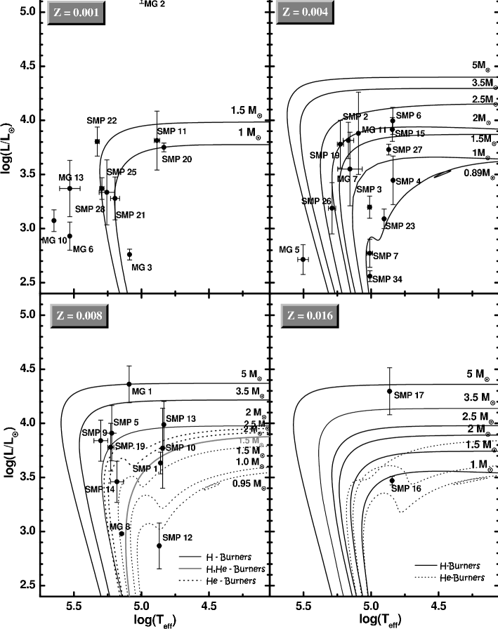
Figure 4: Position of the PNe central stars on the HR diagram. Isochrones are from Vassiliadis & Wood (vassiliadis2 (1994)).

6 The age-metallicity relation

As a first approximation, O, Ne, S, and Ar measured in PNe can be used as tracers of interstellar abundances at the time the progenitor stars were born. Since these elements are generally well correlated with each other, as we have seen in Fig. 2, in the following we will consider oxygen abundances as representative, since the oxygen lines are very bright and the abundances are well determined. Fig. 5 gives the derived age-metallicity relation in the form of oxygen abundances as a function of age. The abundances are defined as [O/H] = log(O/H) – log(O/H)_⊙, as usual, and the solar abundance was taken as log(O/H)_⊙ + 12 = 8.70 (see for example Allende-Prieto et al. allende (2001) and Asplund et al. asplund (2004)). Error bars are included for the oxygen abundances according to the values given in Table 8. Concerning the stellar ages, it is difficult to estimate meaningful uncertainties, but based on the adopted isochrones, a typical error of about $\Delta t\simeq 0.5\,$Gyr can be estimated for ages $t\leq 4\,$Gyr, and of $\Delta t\simeq 2\,$Gyr for older objects.

Figure 5: Oxygen abundances as a function of age. A second order polynomial fit is also included (dashed line). Objects plotted as empty circles are not included in the fit.

The three young objects in Fig. 5 with low oxygen abundances and represented as empty circles are SMP22, SMP25, and SMP28. These nebulae have extremely large N/O ratios, log(N/O) $\simeq 0.8$, compared to the other objects. Since their nitrogen abundance relative to hydrogen is normal, log(N/H)+12 $\simeq 8$, their oxygen abundance is strongly depressed, probably owing to ON cycling in the progenitor star. Therefore these objects should not be included in the determination of the age-metallicity relation.

In order to compare our derived age-metallicity relation with stellar data, it is interesting to convert the [O/H] abundances into [Fe/H] metallicities. Iron cannot be accurately determined from PNe data, in view of the faintness of the Fe lines and the possibility of grain condensation, but average [O/Fe] $\times$ [Fe/H] relationships can be obtained from stellar data or theoretical models. In the range $-2.0<{\rm[Fe/H]}<0.0$ this relationship is approximately linear, so that an [O/H] to [Fe/H] conversion formula can be written as

$${\rm[Fe/H]}\simeq a+b\,{\rm[O/H]}\ .$$ (3)

where $a$ and $b$ are constants in this metallicity range. As an example, the theoretical SMC model by Russell & Dopita (russell (1992)) leads to the coefficients $a\simeq 0.45$ and $b\simeq 1.41$. Alternatively, using the theoretical [O/Fe] $\times$ [Fe/H] relation for the Magellanic Clouds given by Matteucci (matteucci (2000), fig. 6.3), one obtains $a\simeq 0.16$ and $b\simeq 1.27$. Also, using the approximate [O/H] $\times$ age relation for the SMC planetary nebulae, and an [Fe/H] $\times$ age relation obtained from the SMC cluster data of Da Costa & Hatzidimitriou (dacosta1 (1998)), de Freitas Pacheco et al. (pacheco (1998)), Piatti et al. (piatti1 (2001), piatti2 (2005)), and Da Costa (dacosta2 (2002)), we have $a\simeq 0.15$ and $b\simeq 1.28$, very similar to the previous set of coefficients. The corresponding [O/Fe] $\times$ [Fe/H] relation from these sources present a good fit with stellar data from several sources, as can be seen for example from Hill et al. (hill (1997)). Fig. 6a shows the [Fe/H] $\times$ age relationship obtained using Eq. 3 with the constants derived from the [O/Fe] $\times$ [Fe/H] relation for the SMC from Matteucci (matteucci (2000)). The other sets of coefficients mentioned above would lead to a figure very similar to Fig. 6a. Since we would like to compare this relationship with some work done previously to the derivation of the new solar oxygen abundances, we have used in the calibration of Fig. 6 the older solar abundances, namely log (O/H)_⊙ + 12 = 8.93 (cf. Anders & Grevesse anders (1989)). A similar plot based on preliminary results was presented by Idiart et al. (icm2005 (2005)).

Figure 6: [Fe/H] metallicities as a function of age. The solid line shows the results of theoretical models for the SMC by Pagel & Tautvaišiene (pagel (1998)). The data points show (a) the converted [Fe/H] metallicities using the [O/Fe] $\times$ [Fe/H] relationship from Matteucci (matteucci (2000)). (b) the converted [Fe/H] metallicities obtained by calibrating the [O/H] $\times$ [Fe/H] relationship matching the abundances of the youngest objects in our sample and in the models by Pagel & Tautvaišiene (pagel (1998)).

The results of Fig. 5 or Fig. 6 can be conservatively interpreted as a mild decrease of the metallicity with age, as shown by the dashed line, which is a least squares fit to the data adopting a second order polynomial, and not including the objects represented as empty circles. However, a closer look suggests that there is a sharper increase in the abundances in the last 2 Gyr, whereas for ages larger than 3 Gyr the abundances do not change appreciably, which is consistent with a recent burst of star formation. For illustration purposes, Fig. 6 includes the theoretical age-metallicity predicted by the model of Pagel & Tautsvaišiene (pagel (1998)), which clearly indicates a burst in the last 2 to 3 Gyr. It is not our purpose here to fit the observed age-metallicity relation to theoretical models, but it should be mentioned that the agreement between our results and the models by Pagel & Tautvaišiene (pagel (1998)) can be improved by calibrating the oxygen abundances directly with the model input. In this case, we could adopt [Fe/H] $\simeq-0.45$ for the youngest objects as in Pagel & Tautvaišiene (pagel (1998)), which corresponds to log (O/H) + 12 $\simeq 8.54$ in our sample, or [O/H] $\simeq-0.39$ [using log (O/H)_⊙ + 12 = 8.93], so that we would have [O/Fe] $\simeq 0.06$ and the metallicity would be given by [Fe/H] $\simeq$ [O/H] – 0.06, instead of Eq.3. Fig. 6b shows the corresponding age-metallicity relation, which is better adjusted to the data, especially near the burst region at $t<3\,$Gyr.

The presence of bursts in the Magellanic Clouds has already been suggested in some previous work. For instance, in the case of the LMC some signs of star formation bursts can be seen in the age-metallicity relation derived from HST observations of PNe by Dopita et al. (dopita1 (1997), fig. 5) and Dopita (dopita2 (1999)). In this case, a strong burst of star formation was suggested between 1–3 Gyr ago, which increased the metallicity by a factor larger than two. Stellar cluster data also support these conclusions, as can be seen from van den Bergh (vandenbergh (1991)) and Girardi et al. (girardi (1995)). More generally, recent models of Blue Compact Galaxies and dwarf spheroidal galaxies in the Local Group were developed by Lanfranchi & Matteucci (lanfranchi (2003)) who suggested that the former are characterized by several short bursts of star formation separated by long quiescent periods, while for the latter one or two long bursts and efficient stellar winds would be sufficient.

For the SMC, the age distribution of clusters seems to be more homogeneous (cf. van den Bergh vandenbergh (1991)), a result that is supported by the essentially monotonic age-metallicity relation derived by Dolphin et al. (dolphin (2001)) on the basis of SMC clusters and field stars. More recently, Harris & Zaritsky (harris (2004)) determined the global star formation history (SFH) and the age-metallicity relation for the SMC based on their photometric survey. In this case, a distinct increase in the global metallicity occurred in the last 3 Gyr, rising the metallicity from [Fe/H] $\simeq-0.9$ to [Fe/H] $\simeq-0.4$, which is consistent with our results, taking into account the uncertainties in the metallicity determination. As discussed by Harris & Zaritsky (harris (2004)), that period coincided approximately with a past perigalactic passage by the SMC relative to the Milky Way, which may have originated the observed burst. These results are largely consistent with cluster data by Da Costa & Hatzidimitriou (dacosta1 (1998)) and Piatti et al. (piatti1 (2001), piatti2 (2005)). Also, in a recent work, Kayser et al. (kayser (2007)) obtained VLT spectroscopy and HST photometry for a large sample of SMC clusters. Using a [Fe/H] calibration and adopted ages, they derived an age-metallicity relation and found a flat plateau between 2 and 4 Gyr approximately, and a steep rise towards the younger end, which is in excellent agreement with our results shown in Fig. 6. In another recent work on the SFH of the SMC based on cluster data, Noël et al. (noel (2007)) obtained average metallicities at several age intervals for cluster ages $t<13\,$Gyr and found that the mean metallicities of the stars formed in the considered SMC field were about [Fe/H] $\simeq-1.3$ for $t>4\,$Gyr, increasing steadily to the present gas-phase abundance of about [Fe/H] $\simeq-0.5$. Although these results are still preliminary, and represent a limited region of the SMC, it is interesting to note that a very good agreement is obtained with our present results.

7 Conclusions

In this paper we have presented new abundance data on planetary nebulae in the SMC, in order to study the chemical evolution of this galaxy. Spectral line fluxes are given for a sample of 36 nebulae, and the chemical composition is derived for a larger sample of 44 objects. The physical properties of most of the PNe progenitor stars are derived, including the effective temperatures, luminosities, masses, and ages. As a result, an age-metallicity relation was obtained for the SMC, which shows a clear indication of a star formation burst that occurred 2–3 Gyr ago. By the use of a calibration between the Fe and O abundances, this relation can be compared with similar relations obtained recently, acting as an important constraint to chemical evolution models for the SMC.

- (1) Allende-Prieto, C., Lambert, D. L., & Asplund, M. 2001, ApJ, 556, L63
- (2) Aller, L. H. 1984, Physics of thermal gaseous nebulae (Dordrecht: Reidel)
- (3) Aller, L. H., Keyes, C. D., Ross, J. E., & Omara, B. J. 1981, MNRAS, 194, 613
- (4) Anders, E. & Grevesse, N. 1989, Geochim. Cosmochim. Acta 53, 197
- (5) Asplund, M., Grevesse, N., Sauval, A. J., Allende-Prieto, C., & Kiselman, D. 2004, A&A, 417, 751
- (6) Bertelli, G., Mateo, M., Chiosi, C., & Bressan, A. 1992, ApJ, 388, 400
- (7) Boroson, T. A. & Liebert, J. 1989, ApJ, 339, 844
- (8) Cardelli, J. A., Clayton, G. C., & Mathis, J. S. 1989, ApJ, 345, 245
- (9) Cazetta, J. O. & Maciel, W. J. 1994, A&A, 290, 936 ApJ, 345, 245
- (10) Chiappini, C., & Maciel, W. J. 1994, A&A, 288, 921
- (11) Costa, R. D. D., de Freitas Pacheco, J. A., & Idiart, T. P. 2000, A&AS, 145, 467
- (12) Da Costa, G. S. 2002, IAU Symposium 207, Extragalactic Star Clusters, ed. D. Geisler, E. K. Grebel, & D. Minniti, (San Francisco: ASP), 83
- (13) Da Costa, G. S., Hatzidimitriou, D. 1998, AJ, 115, 1934
- (14) de Freitas Pacheco, J. A., Barbuy, B., & Idiart, T. P. 1998, A&A, 332, 19
- (15) Dennefeld, M. 1989, Recent developments of Magellanic Cloud research (Meudon: Observatoire de Paris), ed. K. S. de Boer, F. Spite, & G. Stasińska, 107
- (16) Dolphin, A. E., Walker, A. R., Hodge, P. W., et al. 2001, ApJ, 562, 303
- (17) Dopita, M. A. 1999, New views of the Magellanic Clouds, IAU Symp. 190, ed. Y. -H. Chu, N. B. Suntzeff, J. E. Hesser, & D. A. Bohlander (San Francisco: ASP), 332
- (18) Dopita, M. A., Vassiliadis, E., Wood, P. R., et al. 1997, ApJ, 474, 188
- (19) Dufour, R. J. & Killen, R. M. 1977, ApJ, 211, 68
- (20) Escudero, A. V., Costa, R. D. D., & Maciel, W. J. 2004, A&A, 414, 211
- (21) Feast, M. W. & Walker, A. R. 1987, ARA&A, 25, 345
- (22) Girardi, L., Chiosi, C., Bertelli, G., & Bressan, A. 1995, A&A, 298, 87
- (23) Harries, T., J., Hilditch, R. W., & Howarth, I. D. 2003, MNRAS, 339, 157
- (24) Harris, J., & Zaritsky, D. 2004, AJ, 127, 1531
- (25) Henry, R. B. C., Kwitter, K. B., & Balick, B. 2004, AJ, 127, 2284
- (26) Hill, V., Barbuy, B., & Spite, M. 1997, A&A, 323, 461
- (27) Idiart, T. P., Costa, R. D. D., & Maciel, W. J. 2005, Planetary Nebulae as astronomical tools, ed. R. Szczerba, G. Stasińska, & S. K. Górny (Melville, NY: Am. Inst. of Physics), 261
- (28) Kaler, J. B. & Jacoby, G. H. 1989, ApJ, 345, 871
- (29) Kayser, A., Grebel, E. K., Harbeck, D. R., Cole, A. A., Koch, A., Gallagher, J. S., & Da Costa, G. S. 2007, Globular clusters - guides to galaxies, ed. T. Richtler & S. S. Larsen, (Heidelberg: Spring) (in press) (astro-ph/0607047)
- (30) Keller, S. C., & Wood, P. R. 2006, ApJ, 642, 834
- (31) Kingdon, J., & Ferland, G. J. 1995, ApJ, 442, 714
- (32) Kingsburgh, R. L., & Barlow, M. J. 1994, MNRAS, 271, 257
- (33) Lanfranchi, G., & Matteucci, F. 2003, MNRAS, 345, 71
- (34) Leisy, P. 2006, private communication
- (35) Leisy, P. & Dennefeld, M. 1996, A&AS, 116, 95
- (36) Leisy, P. & Dennefeld, M. 2006, A&A, 456, 451
- (37) Maciel, W. J., Costa, R. D. D., & Idiart, T. P. 2006, Planetary Nebulae beyond the Milky Way, ed. L. Stanghellini, J. R. Walsh, & N. G. Douglas (Heidelberg: Springer), 209
- (38) Maciel, W. J., Quireza, C., & Costa, R. D. D. 2007, A&A, 463, L13
- (39) Matteucci, F. 2000, The chemical evolution of the Galaxy (Dordrecht: Kluwer)
- (40) Meatheringham, S. J., & Dopita, M. A. 1991a, ApJS, 75, 407
- (41) Meatheringham, S. J., & Dopita, M. A. 1991b, ApJS, 76, 1085
- (42) Meatheringham, S. J., Dopita, M. A., & Morgan, D.H. 1988, ApJ, 329, 166
- (43) Meyssonnier, N. 1995, A&AS, 110, 545
- (44) Monk, D. J., Barlow, M. J., & Clegg, R. E. S. 1988, MNRAS, 234, 583
- (45) Noël, N. E. D., Gallart, C., Aparicio, A., Hidalgo, S. L., Carrera, R., Costa, E., & Méndez, R. A. 2007, Stellar populations as building blocks of galaxies, IAU Symp. 241, ed. A. Vazdekis, & R. Peletier, (San Francisco: ASP) (in press)
- (46) Olszewski, E.W., Suntzeff, N.B., & Mateo, M. 1996, ARA&A, 34, 511
- (47) Osmer, P. S. 1976, ApJ, 203, 352
- (48) Osterbrock, D. E. 1989, Astrophysics of Gaseous Nebulae and Active Galactic Nuclei (Mill Valley: University Science Books)
- (49) Pagel, B. E. J.. & Tautvaišiene, G. 1998, MNRAS, 299, 535
- (50) Peimbert, M. 1978, Planetary Nebulae, IAU Symp. 76, ed. Y. Terzian (Dordrecht: Reidel), 215
- (51) Péquignot, D., Petitjean, P., & Boisson, C. 1991, A&A, 251, 680
- (52) Piatti, A. E., Santos, J. F. C., Clariá, J. J., Bica, E., Sarajedini, A., & Geisler, D. 2001, MNRAS, 325, 792
- (53) Piatti, A. E., Sarajedini, A., Geisler, D., Seguel, J., & Clark, D. 2005, MNRAS, 358, 1215
- (54) Richer, M. G., & McCall, M. L. 2006, Planetary Nebulae beyond the Milky Way, ed. L. Stanghellini, J. R. Walsh, & N. G. Douglas (Heidelberg: Springer), 220
- (55) Rola, C. & Stasińska, G. 1994, A&A, 282, 199
- (56) Russell, S. C., & Dopita, M. A. 1992, ApJ, 384, 508
- (57) Stanghellini, L., Shaw, R. A., Balick, B., Mutchler, M., Blades, J. C., & Villaver, E. 2003, ApJ, 596, 997
- (58) Stasińska, G., Richer, M. G., & McCall, M. L. 1998, A&A, 336, 667
- (59) van den Bergh, S. 1991, ApJ, 369, 1
- (60) Vassiliadis, E., Dopita, M. A., Morgan, D. H., & Bell, J. F. 1992, ApJS, 83, 87
- (61) Vassiliadis, E., & Wood, P. R. 1992, ApJS, 92, 125
- (62) Webster, B. L. 1976, MNRAS, 174, 513
- (63) Wood, P. R., Meatheringham, S. J., Dopita, M. A., & Morgan, D. H. 1987, ApJ, 320, 178