Unambiguous coherent state identification: Searching a quantum database

Unambiguous identification of coherent states: Searching a quantum database

Abstract

We consider an unambiguous identification of an unknown coherent state with one of two unknown coherent reference states. Specifically, we consider two modes of an electromagnetic field prepared in unknown coherent states $|\alpha_{1}\rangle$ and $|\alpha_{2}\rangle$, respectively. The third mode is prepared either in the state $|\alpha_{1}\rangle$ or in the state $|\alpha_{2}\rangle$. The task is to identify (unambiguously) which of the two modes are in the same state. We present a scheme consisting of three beamsplitters capable to perform this task. Although we don’t prove the optimality, we show that the performance of the proposed setup is better than the generalization of the optimal measurement known for a finite-dimensional case. We show that a single beamsplitter is capable to perform an unambiguous quantum state comparison for coherent states optimally. Finally we propose an experimental setup consisting of $2N-1$ beamsplitters for unambiguous identification among $N$ unknown coherent states. This setup can be considered as a search in a quantum database. The elements of the database are unknown coherent states encoded in different modes of an electromagnetic field. The task is to specify the two modes that are excited in the same, though unknown, coherent state.

I Introduction

The ability to discriminate quantum states plays an important role in quantum information processing. Because of the quantum interference two (non-orthogonal) quantum states cannot be distinguished perfectly providing the number of copies of these states is limited. The topic of quantum state discrimination was firmly established in 1970s by pioneering work of Helstrom helstrom , who considered a minimum error discrimination of two known quantum states. In this case the state identification is probabilistic. Another equally significant approach is the unambiguous discrimination of quantum states, originally formulated and analyzed by Ivanovic, Dieks and Peres ivanovic ; dieks ; peres in 1987. In contrast to the minimum error discrimination approach, the unambiguous state identification is deterministic, i.e. no erroneous conclusions are permitted. But in addition an inconclusive result is allowed corresponding to situations in which the state identification fails. The solution for unambiguous discrimination of two known pure states appearing with arbitrary prior probabilities (further denoted as $\eta_{1},\eta_{2}$) was obtained by Jaeger and Shimony jaeger . Subsequent research was mainly focused on unambiguous discrimination among several known pure states and unambiguous discrimination of two mixed states, which is still an open problem. The physical implementation of the optimal unambiguous discriminator device working for arbitrary coherent states was proposed by K. Banazsek banaszek .

All results mentioned above are heavily based on a prior classical knowledge we have about those quantum states that are to be discriminated. S. Barnett et al. jex have studied this problem in detail and in addition they have addressed the following intriguing question: Is it possible to say anything unambiguously whether pure quantum states of a pair of identical quantum systems (finite dimensional) are equal or not? Here no prior knowledge about the states is assumed. This problem is called quantum state comparison (for extension to more systems see Ref. jex04 ). It turned out that symmetry with respect to the exchange of the subsystems enables one to reveal unambiguously the difference between the states of the subsystems, however their equality cannot be determined unambiguously. E. Andersson et al. andersson investigated this problem also for coherent states and proposed a simple setup (described in Sec. II), consisting of one beam splitter and a photodetector, capable to perform this task.

Such results stimulated J. Bergou and M. Hillery bergou to reduce the prior knowledge in unambiguous discrimination of quantum states. These authors formulated the following problem: Imagine we are given two qubits $B$ and $C$ each of them in an unknown pure state. At the same time we are given also a third qubit $A$, which is guaranteed to be either in the state of the first or the second qubit. The task is to determine unambiguously with which of the two qubits the state of the third qubit matches. In such modification of the original problem the whole information is conveyed by states of quantum systems. Given the fact that we have just a single copy of each of the two states even the optimal quantum mechanical measurement would allow us to determine those states with a rather small fidelity (for more details see Refs. helstrom ; massar ; derka ). Therefore, instead of trying to estimate reference states we directly use them in their “quantum” form. The control of the behavior of the device by the quantum program register is the key feature of programmable quantum devices nielsen ; hillery01 ; dusek (for a review see Ref. buzek2006 ). In these devices one subsystem serves as the data register and the second quantum subsystem as the program register that carries instructions about transformations the machine has to perform on the data register.

The problem of unambiguous discrimination of unknown states, called also the unambiguous quantum state identification problem (UI), has been investigated over last few years by many authors. Bergou et al. bergou2 examined the situation with more copies of the third qubit $A$. If qudits ($d$ dimensional quantum systems) instead of the qubits are used and more copies of qudits A and B are provided then the analytical solution for equal prior probabilities was obtained by A. Hayashi et al. in Ref. hayashi . C. Zhang and M. Ying zhang investigated the unambiguous identification among $n$ unknown qudit states and they provided necessary and sufficient criterion characterizing all possible programmable discriminators performing this task.

One of the aim of this paper is to illustrate that a prior knowledge of a subset of states ${\cal S}$ uniformly entering subsystems $A$ and $B$ can significantly affect the optimal UI measurement and the performance of it with respect to the universal UI measurement. We illustrate this on two examples: The first example deals with the so called equatorial qubits described in Sec. II.B. The second example deals with coherent states examined in Sec. IV. In Sec. III we present how an “intuitive” universal UI measurement of systems of an arbitrary dimension can be constructed. Further we will compare different types of UI devices with the optimal universal one found in Ref. hayashi . Although the UI measurement of coherent states will not be proved to be optimal, we will show that it rapidly outperforms the universal UI measurement. In addition we will show that in the case of continuous variable when the inputs are represented by coherent states the UI measurement can be also easily implemented by three beam splitters and two photo-detectors.

Formally the unambiguous identification problem (UI) fits into the following framework: Three identical subsystems A,B and C are prepared in unknown pure product states $|\psi_{?}\rangle_{A}$, and $|\psi_{1}\rangle_{B},|\psi_{2}\rangle_{C}$, respectively. Furthermore, the subsystem A is guaranteed to be either in the same state as the subsystem B or as the subsystem C. Thus two types of states should be discriminated:

$$|\Psi_{1}\rangle_{ABC}\equiv|\psi_{1}\rangle_{A}\otimes|\psi_{1}\rangle_{B}\otimes|\psi_{2}\rangle_{C}\,,$$

$$|\Psi_{2}\rangle_{ABC}\equiv|\psi_{2}\rangle_{A}\otimes|\psi_{1}\rangle_{B}\otimes|\psi_{2}\rangle_{C}\,.$$ (1)

The unambiguous identification machine is described by means of a positive operator value measure (POVM) consisting of three elements $\{E_{0},E_{1},E_{2}\}$. Element ${\rm E}_{1}$ (respectively ${\rm E}_{2}$) corresponds to correct identification of $|\Psi_{1}\rangle$ (respectively $|\Psi_{2}\rangle$) type of state and ${\rm E}_{0}$ corresponds to the inconclusive result. These elements must obey no-error conditions [Eq.(2)] and constitute a proper POVM [Eq.(3)]:

$$Tr[{\rm E}_{1}\rho_{2}]=Tr[{\rm E}_{2}\rho_{1}]=0\,;\quad\rho_{i}=|\Psi_{i}\rangle\langle\Psi_{i}|\,;$$ (2)

$${\rm E}_{i}\geq 0,{\rm E}_{0}\geq 0\,;\quad{\rm E}_{0}+{\rm E}_{1}+{\rm E}_{2}={\openone}\,.$$ (3)

It is assumed that the state $|\Psi_{1}\rangle$ ($|\Psi_{2}\rangle$) appears with a prior probability $\eta_{1}$ ($\eta_{2}$). The performance of the UI measurement is quantified by a probability of identification for a particular choice of states

$$P(|\psi_{1}\rangle,|\psi_{2}\rangle)=\eta_{1}Tr[{\rm E}_{1}\rho_{1}]+\eta_{2}Tr[{\rm E}_{2}\rho_{2}]\,.$$ (4)

Although $P(|\psi_{1}\rangle,|\psi_{2}\rangle)$ is not a measurable quantity in the problems we consider, it will be very useful for comparison of different UI measurements. Alternatively, we can use the average value to evaluate the performance of UI devices

$$\overline{P(S)}=\int_{S}\int_{S}P(|\psi_{1}\rangle,|\psi_{2}\rangle)\quad d\psi_{1}d\psi_{2}\,.$$ (5)

In what follows we will denote the set of all pure states of a $d$-dimensional quantum system (qudit) by $S_{d}$ and the subscript of $P$ will indicate the used UI measurement. The optimality of UI measurements is defined with respect to their average performance, i.e. the aim is to optimize $\overline{P(S)}$.

II Unambiguous Identification for qubits

The solution to the unambiguous identification problem for a qubit was given in Ref. bergou . The optimal UI measurement depends only on prior probabilities $\eta_{1}=\eta$, $\eta_{2}=1-\eta$. Specifically, there are three different regions of values of $\eta$ for which the POVM operators are specified as follows:

$$\begin{array}[]{cll}0\leq\eta<\frac{1}{5}:&{\rm E}^{opt}_{1}=0\,;&{\rm E}^{opt}_{2}={\openone}_{C}\otimes\psi^{-}_{AB}\,;\\ \frac{1}{5}\leq\eta\leq\frac{4}{5}\,:&{\rm E}^{opt}_{1}=\lambda{\openone}_{B}\otimes\psi^{-}_{AC}\,;&{\rm E}^{opt}_{2}=\frac{4-4\lambda}{4-3\lambda}{\openone}_{C}\otimes\psi^{-}_{AB}\,;\\ \frac{4}{5}<\eta\leq 1\,:&{\rm E}^{opt}_{1}={\openone}_{B}\otimes\psi^{-}_{AC}\,;&{\rm E}^{opt}_{2}=0\,,\end{array}$$

where $|\psi^{-}_{AB}\rangle=1/\sqrt{2}(|01\rangle-|10\rangle)_{AB}$, $\lambda=\frac{2}{3}(2-\sqrt{\frac{\eta_{2}}{\eta_{1}}})$ and $|\psi^{-}_{AB}\rangle\langle\psi^{-}_{AB}|=\psi_{AB}^{-}\equiv{\rm ASym}_{AB}$ is a projector onto the antisymmetric part of the two qubit Hilbert space ${\cal H}^{\otimes 2}_{2}$. The inconclusive result is associated with the POVM element ${\rm E}^{opt}_{0}={\openone}-{\rm E}^{opt}_{1}-{\rm E}^{opt}_{2}$.

II.1 Relation to quantum state comparison

Intuitively, the unambiguous state comparison and the unambiguous state identification are very closely related problems. Indeed, one can consider the following family of problems: given $n+1$ qudits in unknown states $\psi_{1},\dots,\psi_{n},\psi_{n+1}$. All qudits [except the $(n+1)$-th one] are guaranteed to be in different states. Decide whether $(n+1)$-th qudit matches with one of the given qudits, or not. The unambiguous state comparison jex is a task with $n=1$ and unambiguous identification corresponds to $n=2$ providing that the $(n+1)$-th qudit is promised to be in one of the states $\psi_{1},\dots,\psi_{n}$. Moreover, the identification can be logically reduced to a series of state comparisons, although such reduction does not necessarily give an optimal identification scheme. In particular, the UI measurement for $n=2$ can be always designed out of the unambiguous comparison device in the following way: The experimentalist randomly chooses (with probabilities $q$ and $1-q$, respectively) one of the reference states ($|\psi_{B}\rangle,|\psi_{C}\rangle$) to be the input of the unambiguous comparator machine together with the unknown state $|\psi_{A}\rangle$. Performing the state comparison $M_{AB}$ ($M_{AC}$) the conclusive result means that the unknown state is $|\psi_{C}\rangle$ ($|\psi_{B}\rangle$) Formally this corresponds to a probabilistic switching between two measurement apparatuses resulting in the UI measurement consisting of POVM elements $\overline{E}_{1}=qI_{B}\otimes F^{\rm dif}_{AC}$, $\overline{E}_{2}=(1-q)I_{C}\otimes F^{\rm dif}_{AB}$, $\overline{E}_{0}=I-\overline{E}_{1}-\overline{E}_{2}$, where $F^{\rm dif}$ denotes the POVM element associated with the conclusive result saying that two states are different jex .

For a prior probability $\eta_{1}<\frac{1}{5}$ the optimal qubit UI measurement is projective, distinguishing the antisymmetric and symmetric states of the subsystem $AB$. Moreover, the qubit $C$ is not used at all, and the exchange symmetry of the states with respect to systems $A$ and $B$ is measured distinguishing between the states $|\psi_{1}\rangle_{A}\otimes|\psi_{1}\rangle_{B}$ and $|\psi_{2}\rangle_{A}\otimes|\psi_{1}\rangle_{B}$. This is exactly the aim of a quantum state comparison of two unknown pure states. States of the type $|\psi\rangle\otimes|\psi\rangle$ are from the symmetric subspace, therefore the projection onto the antisymmetric subspace unambiguously identifies whether the states of the subsystems are different. On the other hand projection onto the symmetric subspace is inconclusive, because both types of states $|\psi\rangle\otimes|\psi\rangle$, $|\psi\rangle\otimes|\phi\rangle$ have nonzero overlap with it. Analogous considerations holds also for the interval $\eta_{1}>\frac{4}{5}$ and a subsystem AC. For the aforementioned prior probabilities the mean probability of identification equals $\overline{P_{opt}(S_{2})}=\eta_{\min}/4$, where $\eta_{\min}=\min\{\eta_{1},\eta_{2}\}\in[0,1/5]$ and $S_{2}$ denotes the set of all pure states of the qubit.

For equal prior probabilities the optimal measurement is a “true” POVM measurement, whose elements ${\rm E}^{opt}_{1}$, ${\rm E}^{opt}_{2}$ are $2/3$ times the above-mentioned quantum state comparison measurement elements ${\rm ASym}_{AC}$, ${\rm ASym}_{AB}$. In this case the mean probability of identification $\overline{P_{opt}(S_{2})}$ is $1/6$. Using the mixing strategy the success probability can reach at most $1/8$.

II.2 Unambiguous identification of equatorial qubits

Let us consider a restricted set of pure states lying on the equator of the Bloch sphere $|\varphi\rangle=1/\sqrt{2}(|0\rangle+e^{\imath\varphi}|1\rangle)$ with $\varphi\in[0,2\pi)$. Let us denote the subset of all equatorial states by $S_{eq}$. We are going to find the UI measurement, which optimizes the probability of identification $\overline{P_{eq}(S_{eq})}$ averaged over the set $S_{eq}$. Following the approach used in Ref. bergou2 we obtain

$$\overline{P_{eq}(S_{eq})}=\eta_{1}Tr[{\rm E}^{eq}_{1}\Omega_{1}]+\eta_{2}Tr[{\rm E}^{eq}_{2}\Omega_{2}]\,,$$ (6)

with average states

$$\Omega_{j}=\frac{1}{(2\pi)^{2}}\int_{0}^{2\pi}\int_{0}^{2\pi}\varphi_{j}\otimes\varphi_{1}\otimes\varphi_{2}\quad d\varphi_{1}d\varphi_{2}\,,$$ (7)

where we used the notation $\varphi_{j}=|\varphi_{j}\rangle\langle\varphi_{j}|$. After a little algebra this yields

$$\Omega_{1}=\frac{1}{8}{\openone}_{C}\otimes(|00\rangle\langle 00|+|11\rangle\langle 11|+2|\psi^{+}\rangle\langle\psi^{+}|)_{AB}\,;$$ (8)

$$\Omega_{2}=\frac{1}{8}{\openone}_{B}\otimes(|00\rangle\langle 00|+|11\rangle\langle 11|+2|\psi^{+}\rangle\langle\psi^{+}|)_{AC}\,,$$

with $|\psi^{+}\rangle=\frac{1}{\sqrt{2}}(|01\rangle+|10\rangle)$. We integrate the no-error conditions (2) in the same way and obtain $Tr[{\rm E}^{eq}_{1}\Omega_{2}]=Tr[{\rm E}^{eq}_{2}\Omega_{1}]=0$. Operators ${\rm E}^{eq}_{j}$, $\Omega_{j}$ are positive therefore the previous equation means that the operators in the trace have orthogonal supports. Thus we determine the zero eigenvectors of the opeators $\Omega_{1}$ and $\Omega_{2}$, $\Omega_{2}|a_{j}\rangle=0$ and $\Omega_{1}|b_{j}\rangle=0$, respectively, where

$$|a_{1}\rangle=|0\rangle_{B}\otimes|\psi_{AC}^{-}\rangle\,;\quad|b_{1}\rangle=|0\rangle_{C}\otimes|\psi_{AB}^{-}\rangle\,;$$ (9)

$$|a_{2}\rangle=|1\rangle_{B}\otimes|\psi_{AC}^{-}\rangle\,;\quad|b_{2}\rangle=|1\rangle_{C}\otimes|\psi_{AB}^{-}\rangle\,.$$

These eigenvectors determine subspaces in which POVM elements ${\rm E}^{eq}_{2}$, ${\rm E}^{eq}_{1}$

$${\rm E}^{eq}_{1}=\sum^{2}_{j,k=1}\alpha_{jk}|a_{j}\rangle\langle a_{k}|\,;\quad{\rm E}^{eq}_{2}=\sum^{2}_{j,k=1}\beta_{jk}|b_{j}\rangle\langle b_{k}|$$ (10)

can operate. Our goal is to maximize $\overline{P_{eq}(S_{eq})}$, while keeping the POVM elements positive. Therefore we use equations (8) and (10) to express equation (6) only in terms of the coefficients $\alpha_{jk}$, $\beta_{jk}$

$$\overline{P_{eq}(S_{eq})}=\frac{\eta_{1}}{8}(\alpha_{11}+\alpha_{22})+\frac{\eta_{2}}{8}(\beta_{11}+\beta_{22})\,.$$ (11)

Accidentally at the same time the expression for $\overline{P_{eq}(S_{eq})}$ coincides with $\overline{P_{opt}(S_{2})}$ and the states $|a_{j}\rangle$, $|b_{k}\rangle$ are the same as in Ref. bergou2 [compare with Eqs. (3.19-3.22) of this reference]. Therefore the optimization task and the resulting measurement is in our case exactly the same as for the universal UI of qubits. As a result we see that the optimal UI measurement for equatorial states is the same as for the most general qubit state (specified at the beginning of this section). Hence, in this case the a priori knowledge does not help us to improve the performance of the UI measurement.

III Unambiguous Identification of Qudits

III.1 The Swap-based approach

The POVM elements for the optimal universal UI of qubits ${\rm E}^{opt}_{1},{\rm E}^{opt}_{2}$ are proportional to the projectors onto the antisymmetric subspace of the two-qubit subsystems AC and AB, respectively. The simple generalization of the aforementioned universal UI measurement to the case of qudits is the following POVM, which we abbreviate by $sb$ (stands for the “swap-based”):

$${\rm E}^{sb}_{1}=c_{1}{\openone}_{B}\otimes{\rm ASym}_{AC}=c_{1}\frac{1}{2}(1-{\rm Swap_{AC}})\,;$$ (12)

$${\rm E}^{sb}_{2}=c_{2}{\openone}_{C}\otimes{\rm ASym}_{AB}=c_{2}\frac{1}{2}(1-{\rm Swap_{AB}})\,;$$

$${\rm E}^{sb}_{0}={\openone}-{\rm E}^{sb}_{1}-{\rm E}^{sb}_{2},$$

where ${\rm ASym}_{XY}$ denotes the projector to the antisymmetric subspace of $X$ and $Y$ particle.

The positivity of ${\rm E}^{sb}_{0},{\rm E}^{sb}_{1},{\rm E}^{sb}_{2}$ results in the conditions for $c_{1},c_{2}$. Namely, from ${\rm E}^{sb}_{1}\geq 0,{\rm E}^{sb}_{1}\geq 0$ we obtain that $c_{1}\geq 0$ and $c_{2}\geq 0$, whereas the inequality imposed by the positivity of ${\rm E}^{sb}_{0}$ is not so apparent. Further we will calculate eigenvalues of ${\rm E}^{sb}_{0}$ explicitly. Let $\{|\,j\,\rangle\}_{j=1}^{d}$ be a basis of the qudit Hilbert space ${\cal H}_{d}$. Then $|ijk\rangle\equiv|i\rangle_{A}\otimes|j\rangle_{B}\otimes|k\rangle_{C}$ is the basis of the three-qudit Hilbert space ${\cal H}^{\otimes 3}_{d}$. The operator $E^{sb}_{0}$ can be expressed in terms of the identity and the ${\rm Swap}$ operators so $\langle ijk|{\rm E}^{sb}_{0}|lmn\rangle\equiv 0$ whenever $\{ijk\}$ is not a permutation of $\{lmn\}$, i.e. $ijk\neq\sigma(lmn)$. In other words if we properly reorder the above basis the matrix ${\rm E}^{sb}_{0}$ is block diagonal. The blocks are of the following three types:

• the trivial $1\times 1$ block $\langle iii|{\rm E}^{sb}_{0}|iii\rangle=1$

• the $3\times 3$ block with the matrix $\langle\sigma_{1}(iij)|{\rm E}^{sb}_{0}|\sigma_{2}(iij)\rangle$

• the $6\times 6$ block with the matrix $\langle\sigma_{1}(ijk)|{\rm E}^{sb}_{0}|\sigma_{2}(ijk)\rangle$.

The dimensionalities of the blocks are given by the number of inequivalent permutations $\sigma$ of the three indexes.

For qubits only the blocks of the first two types occur in the matrix ${\rm E}^{sb}_{0}$ whereas for qudits $(d>2)$ blocks of all three types arise. Hence we reduced the problem of finding the eigenvalues of the positive operator ${\rm E}^{sb}_{0}$ to an evaluation of the eigenvalues of the matrices mentioned above, which is treated in more details in Appendix A. It is shown there that the positivity of ${\rm E}^{sb}_{0}$ imposes a particularly simple inequality

$$c_{1}+c_{2}\leq 1$$ (13)

regardless of the dimension $d$ ($d>2$).

The probability $(\ref{pidentify})$ reads

$$P_{sb}(|\psi_{1}\rangle,|\psi_{2}\rangle) = \eta_{1}\langle\Psi_{1}|{\rm E}^{sb}_{1}|\Psi_{1}\rangle_{ABC}+\eta_{2}\langle\Psi_{2}|{\rm E}^{sb}_{2}|\Psi_{2}\rangle_{ABC}$$ (14)

$$= \frac{\eta_{1}c_{1}+\eta_{2}c_{2}}{2}(1-|\langle{\psi_{1}}|\psi_{2}\rangle|^{2})\,.$$

Depending on the prior probabilities $\eta_{1},\eta_{2}$ the values of $c_{1},c_{2}$ maximizing $P_{sb}(|\psi_{1}\rangle,|\psi_{2}\rangle)$ read: $c_{1}=0$, $c_{2}=1$ for $\eta_{1}<\eta_{2}$, $c_{1}=1$, $c_{2}=0$ for $\eta_{1}>\eta_{2}$ and $c_{1}+c_{2}=1$ for $\eta_{1}=\eta_{2}$. Hence for equal prior probabilities the swap-based UI measurement is independent of the particular choice of $c_{1}$ and $c_{2}$, i.e.

$$P_{sb}(|\psi_{1}\rangle,|\psi_{2}\rangle)=\frac{1}{4}(1-|\langle{\psi_{1}}|\psi_{2}\rangle|^{2}).$$ (15)

However due to symmetry reasons we will further consider $c_{1}=c_{2}=1/2$ in the case $\eta_{1}=\eta_{2}$, which gives

$${\rm E}^{sb}_{1}=\frac{1}{2}{\openone}_{B}\otimes{\rm ASym}_{AC},\quad{\rm E}^{sb}_{2}=\frac{1}{2}{\openone}_{C}\otimes{\rm ASym}_{AB}\,.$$ (16)

Averaging over the Bloch sphere and using the identity $\int\int_{S_{d}}|\langle{\psi_{1}}|\psi_{2}\rangle|^{2}d\psi_{1}d\psi_{2}=1/d$ zyckowski we obtain the average probability for the swap-based UI machines

$$\overline{P_{sb}(S_{d})}=\frac{1}{4}\left(\frac{d-1}{d}\right)\,.$$ (17)

Although the probabilities itself are independent of the dimension the average value converges to $1/4$ in the limit of $d\to\infty$. This corresponds to an intuitive expectation that two randomly chosen unit vectors in ${\cal H}_{d}$ are more likely to be orthogonal for higher values of $d$.

III.2 Optimal measurement

Although POVM elements ${\rm E}^{sb}_{1},{\rm E}^{sb}_{2}$ proportional to projectors onto the antisymmetric parts of the subsystem AC respectively AB, intuitively seem to be the best universal UI measurement, it was shown by A. Hayashi et al. hayashi that this is not the case for $\eta_{1}=\eta_{2}=\eta=1/2$. The maximization of the average probability $\overline{P_{opt}(S_{d})}$ can be done by exploiting symmetry via joint representations of the unitary group $U\otimes U\otimes U$ ($U\in U(d)$) and the permutation group $S(3)$ permuting the subsystems $A$,$B$ and $C$ of ${\cal H}^{\otimes 3}_{d}$. In our case Hayashi’s optimal POVM measurement can be written explicitly in the form hayashi

$${\rm E}^{opt}_{1} = e{\openone}_{B}\otimes{\rm ASym}_{AC}\,;$$

$${\rm E}^{opt}_{2} = e{\openone}_{C}\otimes{\rm ASym}_{AB}\,,$$ (18)

where $e=\sum_{\lambda}e_{\lambda}\Gamma_{\lambda}$ is a specific operator. The parameter $\lambda$ specifies both $U(d)$ and $S(3)$ irreducible representation, $\Gamma_{\lambda}$ is the projector onto that invariant subspace of ${\cal H}^{\otimes 3}_{d}$, and $e_{\lambda}$ are non-negative real numbers. In our case only two irreducible $U(d)$ representations specified by Young tableaux $\lambda=(2,1,0,\ldots,0)$, $\lambda=(1,1,1,\ldots,0)$ are relevant. The corresponding $e_{\lambda}$’s are $2/3$ and $1/2$. Therefore we have

$$e=\frac{2}{3}\Gamma_{(2,1,0,\ldots,0)}+\frac{1}{2}\Gamma_{(1,1,1,\ldots,0)}.$$ (19)

The projectors $\Gamma_{(2,1,0,\ldots,0)}$ and $\Gamma_{(1,1,1,\ldots,0)}$ project onto the subspaces $(V_{S}\oplus V_{AS})^{\perp}$ and $V_{AS}$, respectively, where $V_{S}$ ($V_{AS}$) is the totally symmetric (antisymmetric) subspace of ${\cal H}^{\otimes 3}_{d}$. Operators ${\openone}_{C}\otimes{\rm ASym}_{AB}$, ${\openone}_{B}\otimes{\rm ASym}_{AC}$ do not mix the subspaces $(V_{S}\oplus V_{AS})^{\perp}$ and $V_{AS}$ on which the operator $e$ acts only a multiple of the identity, i.e. $e|_{V_{AS}}=e|_{(V_{S}\oplus V_{AS})^{\perp}}={\openone}$. Therefore ${\rm E}^{opt}_{1}$ (analogously ${\rm E}^{opt}_{2}$) is essentially $\frac{2}{3}{\openone}_{B}\otimes{\rm ASym}_{AC}$ except for $V_{AS}$, where it is $\frac{1}{2}{\openone}_{B}\otimes{\rm ASym}_{AC}$. Furthermore the POVM elements ${\rm E}^{opt}_{1}$, ${\rm E}^{opt}_{2}$ acting on the totally antisymmetric subspace $V_{AS}$ do not contribute to $P_{opt}(|\psi_{1}\rangle,|\psi_{2}\rangle)$ and $\overline{P_{opt}(S_{d})}$, because input states $|\Psi_{j}\rangle_{ABC}$ [ see Eq. (1)] are symmetric in a pair of subsystems. Thus for calculation of probabilities of identification we can as well use the operators ${\rm E}_{1}=\frac{2}{3}{\openone}_{B}\otimes{\rm ASym}_{AC}=\frac{4}{3}{\rm E}^{sb}_{1}$, ${\rm E}_{2}=\frac{2}{3}{\openone}_{C}\otimes{\rm ASym}_{AB}=\frac{4}{3}{\rm E}^{sb}_{2}$. Hence, in the optimal case

$$P_{opt}(|\psi_{1}\rangle,|\psi_{2}\rangle) = \frac{1}{3}(1-|\langle{\psi_{1}}|\psi_{2}\rangle|^{2})\,,$$ (20)

$$\overline{P_{opt}(S_{d})} = \frac{1}{3}\frac{d-1}{d}\,.$$ (21)

IV Unambiguous Identification of coherent states

Unlike previous sections, where we have considered an unambiguous identification of quantum states from a finite-dimensional Hilbert space ${\cal H}_{d}$, here we work with a semi-infinite dimensional Hilbert space of a linear harmonic oscillator ${\cal H}_{\infty}$, which models a single mode of an electromagnetic field (EM). The techniques presented in Sec. III for qudits work for any dimension $d$. The resulting POVM elements are expressed via constant multiples of projectors, which in large $d$ limit define projectors on ${\cal H}_{\infty}^{\otimes 3}$. Therefore we have formally the same universal UI measurement also for states from ${\cal H}_{\infty}$ and this measurement is optimal for the case of equal prior probability $\eta_{1}=\eta_{2}$.

Our goal in this section is to show that an unambiguous identification of coherent states can be done with much better probability of identification than the optimal UI for all pure states from ${\cal H}_{\infty}$. The basic intuition for this is that coherent states form a very small subset $S_{coh}$ of all pure states from ${\cal H}_{\infty}$ and thus there could be a better way to identify them. The more reasonable motivation is based on the following observation. As it was mentioned in Sec. II.1 for a special choice of the parameters $\eta_{1},\eta_{2}$ the optimal POVM for qubits coincides with the optimal quantum state comparison measurement. Hence if there is a better quantum state comparison of coherent states, which can be used to design an UI setup for coherent states then this setup could perform better than the universal UI measurement identifying all states from ${\cal H}_{\infty}$. E. Andersson et al. andersson proposed such a quantum state comparison setup, which is also simply realizable by a beamsplitter and a photodetector. In what follows we will explain how their setup works. In addition, we will present a proof that it performs optimal quantum state comparison of coherent states. Then we will show how it can be used to design an unambiguous identification setup for coherent states.

IV.1 Quantum comparison of coherent states

A coherent state $|\alpha\rangle$ is fully specified by a complex amplitude $\alpha$. It is a pure state $|\alpha\rangle\in{\cal H}_{\infty}$, which is an eigenstate of the annihilation operator $a|\alpha\rangle=\alpha|\alpha\rangle$. A beamsplitter is a passive-optics device acting on a pair of EM field modes. Its action is described by the Hamiltonian $H=i\theta(ab^{\dagger}-a^{\dagger}b)$ generating the unitary transformation $U=e^{\theta t(ab^{\dagger}-a^{\dagger}b)}$, where $a,a^{\dagger},b,b^{\dagger}$ are creation and annihilation operators of the two modes. The operation of the beamsplitter is particularly simple for coherent states and is determined by the interaction time, i.e. by the transmittivity $T$ and the reflectivity $R$ of the beamsplitter:

$$|\alpha\rangle\otimes|\beta\rangle\mapsto|\sqrt{T}\alpha+\sqrt{R}\beta\rangle\otimes|-\sqrt{R}\alpha+\sqrt{T}\beta\rangle$$ (22)

with $T+R=1$. In comparison of coherent states we want to unambiguously distinguish between $|\alpha\rangle=|\beta\rangle$ and $|\alpha\rangle\neq|\beta\rangle$. This is equivalent to distinguishing $\beta-\alpha=0$ and $\beta-\alpha\neq 0$, which can be done by 50/50 beamsplitter ($T=R=1/2$) in the following way. The state of the second mode after passing through the beamsplitter will be either the vacuum $|0\rangle$ or the state $|\frac{1}{\sqrt{2}}(\beta-\alpha)\rangle$ when $\alpha\neq\beta$. Thus if we detect at least one photon in the second mode, which happens with probability $1-|\langle{0}|\frac{1}{\sqrt{2}}(\beta-\alpha)\rangle|^{2}=1-e^{-\frac{1}{2}|\alpha-\beta|^{2}}$, we are sure that the states were different. The detection of no photons is inconclusive, because all coherent states have a nonzero overlap with the vacuum.

Now we are going to prove optimality of this setup serving as unambiguous coherent state comparator. First we derive the optimal quantum state comparison measurement for coherent states. In general it is a POVM with two elements ${\rm\Pi}^{opt}_{0}$ (inconclusive result) and ${\rm\Pi}^{opt}_{1}$ (unambiguously indicating the inequality of states) obeying the following equations:

$${\rm Tr}\Big{[}{\rm\Pi}^{opt}_{1}|\alpha\rangle_{X}\langle\alpha|\otimes|\alpha\rangle_{Y}\langle\alpha|\Big{]}=0\,;\ \ \ \ \forall\alpha\,,$$ (23)

$${\rm\Pi}^{opt}_{0}\geq 0,\quad{\rm\Pi}^{opt}_{1}\geq 0\,;\quad{\rm\Pi}^{opt}_{0}+{\rm\Pi}^{opt}_{1}={\openone}.$$ (24)

Integrating the no-error condition (23) over all coherent states we obtain the following condition

$$0 = \int_{\mathbb{C}}d\alpha{\rm Tr}\Big{[}{\rm\Pi}^{opt}_{1}|\alpha\rangle\langle\alpha|\otimes|\alpha\rangle\langle\alpha|\Big{]}={\rm Tr}[{\rm\Pi}^{opt}_{1}\Delta]$$ (25)

which defines the operator $\Delta$. The no-error conditions given by (23) are completely equivalent to Eq. (25), because the trace under the integral is nonnegative. The operators ${\rm\Pi}^{opt}_{1}$ and $\Delta$ are positive and therefore Eq. (25) means that these two operators have orthogonal supports. Hence the largest possible support the operator ${\rm\Pi}^{opt}_{1}$ can have is the orthogonal complement to the support of $\Delta$. It is possible to show that

$$\Delta = \frac{\pi}{2}\sum^{\infty}_{N=0}(|\chi_{N}\rangle\langle\chi_{N}|),$$ (26)

where the vectors $|\chi_{N}\rangle=2^{-\frac{N}{2}}\sum^{N}_{k=0}\sqrt{\binom{N}{k}}|k\rangle\otimes|N-k\rangle$ are mutually orthonormal, i.e. $\langle{\chi_{N}}|\chi_{M}\rangle=\delta_{N,M}$ The calculation of $\Delta$ is described in detail in Appendix B.

Moreover the normalized operator $\frac{2}{\pi}\Delta$ is a projector with the same support as $\Delta$. The support of the projector ${\openone}-\frac{2}{\pi}\Delta$ is therefore the largest possible support of ${\rm\Pi}^{opt}_{1}$. The optimal measurement must maximize the probability of revealing the difference of the states launched into the comparator:

$$P_{R}(|\alpha\rangle,|\beta\rangle)={\rm Tr}[{\rm\Pi}^{opt}_{1}|\alpha\rangle\langle\alpha|\otimes|\beta\rangle\langle\beta|]\,,$$ (27)

while keeping the positivity ($0\leq{\rm\Pi}^{opt}_{1}\leq{\openone}$) and the no-error conditions satisfied. Combining these two conditions on the support of ${\rm\Pi}^{opt}_{1}$ yields ${\rm\Pi}^{opt}_{1}={\openone}-\frac{2}{\pi}\Delta$. Thus the optimal unambiguous coherent state comparison is acomplished by the following projective measurement

$${\rm\Pi}^{opt}_{0} = \frac{2}{\pi}\Delta=\sum^{\infty}_{N=0}(|\chi_{N}\rangle\langle\chi_{N}|)_{XY}\,;$$

$${\rm\Pi}^{opt}_{1} = {\openone}-\sum^{\infty}_{N=0}(|\chi_{N}\rangle\langle\chi_{N}|)_{XY}\,.$$ (28)

Now it is sufficient to show that the described quantum state comparison setup performs the measurement (28). The mathematical description of the setup is simple. First the beamsplitter acts on the modes $X$ and $Y$ via a unitary transformation $U(\theta=\pi/4)$ and then the photodetector discriminate between the zero-registered-photon result ${\rm\Pi}^{d}_{0}={\openone}_{X}\otimes(|0\rangle\langle 0|)_{Y}$ and the at-least-one-registered photon ${\rm\Pi}^{d}_{1}={\openone}_{X}\otimes({\openone}-|0\rangle\langle 0|)_{Y}$ in the mode Y. Hence the measurement performed by the setup is given as

$${\rm\Pi}^{bs}_{j}=U^{\dagger}{\rm\Pi}^{d}_{j}U\,;\quad j=0,1\,.$$ (29)

Unitarity of $U$ guarantees that ${\rm\Pi}^{bs}_{j}$ form a projective measurement as well as ${\rm\Pi}^{d}_{j}$. Therefore it suffice to show the equality ${\rm\Pi}^{bs}_{0}={\rm\Pi}^{opt}_{0}$. It follows that

$${\rm\Pi}^{bs}_{0}=\sum^{\infty}_{N=0}U^{\dagger}(|N\rangle_{X}\otimes|0\rangle_{Y}{}_{X}\langle N|\otimes{}_{Y}\langle 0|)U$$ (30)

and the proof is concluded by showing that $U^{\dagger}|N\rangle_{X}\otimes|0\rangle_{Y}=|\chi_{N}\rangle_{XY}$. The technical details are placed in Appendix C.

IV.2 UI measurement with beamsplitters

For the case of a qubit (Sec. II) we have seen explicitly that the unambiguous identification is very closely related to the problem of the state comparison. In some sense the identification seems to consist of two state comparisons performed somehow simultaneously in a single run. However, because only a single copy of the unknown state is available, a very specific “cloning” machine should be used in order to make such reduction of the identification problem possible. Usually the cloning machines buzek1996 distributes the original quantum information (represented by quantum state) among several quantum systems rosko . Such approach results in a complicated entangled state such that the individual systems are described by density matrices on average “closest” to the original quantum state. Unfortunately such cloning cannot be used for our purposes. The potential clones described by mixed quantum states cannot be unambiguously compared with pure states. Therefore we need a very specific cloning machine producing the clones in pure states, i.e. $|\psi\rangle\otimes|0\rangle\otimes|0\rangle_{\rm ancilla}\to|\psi^{\prime}\rangle\otimes|\psi^{\prime}\rangle\otimes|\phi(\psi)\rangle_{\rm ancilla}$. The cloning of coherent states has been analyzed in braunstein , where it was shown that the single beamsplitter assisted by a linear amplifier is optimal. Without the linear amplifier the beamsplitter alone performs on coherent states the transformation $|\alpha\rangle\otimes|0\rangle\to|\sqrt{T}\alpha\rangle\otimes|\sqrt{R}\alpha\rangle$, where $R,T$ stands for reflectivity and transmittivity of the beamsplitter. And this is exactly a type of cloning we are looking for. Hence, the idea is to use one beamsplitter to clone the system $A$ into two modes and afterwards use another two beamsplitters for particular state comparisons. Hence, in addition to the modes A,B,C we add an ancillary mode D set initially to vacuum, i.e. $|\Phi_{in}\rangle=|{\rm\alpha_{?}}\rangle_{A}\otimes|\alpha_{1}\rangle_{B}\otimes|\alpha_{2}\rangle_{C}\otimes|0\rangle_{D}$, where $|{\rm\alpha_{?}}\rangle$ is guaranteed to be either $|\alpha_{1}\rangle$ or $|\alpha_{2}\rangle$.

Our setup is composed of three beamsplitters the action of which is described by the unitary transformation

$$|\Phi_{in}\rangle\mapsto U_{3}(DC)U_{2}(BA)U_{1}(DA)|{\rm\alpha_{?}}\rangle|\alpha_{1}\rangle|\alpha_{2}\rangle|0\rangle\,,$$ (31)

where $U_{j}(XY)$ is associated with the $j$-th beamsplitter acting on the modes X and Y. The first beamsplitter $B_{1}$ (with the transmittivity $T_{1}$) prepares two clones of the unknown state $|\alpha_{j}\rangle_{A}$ that is encoded in the mode $A$

$$|0\rangle_{D}\otimes|{\rm\alpha_{?}}\rangle_{A}\mapsto|\sqrt{R_{1}}{\rm\alpha_{?}}\rangle_{D}\otimes|\sqrt{T_{1}}{\rm\alpha_{?}}\rangle_{A}.$$ (32)

The output system remains in a product state, hence the beamsplitters $B_{2}$ and $B_{3}$ can be analyzed separately

$$B_{2}:|\alpha_{1}\rangle_{B}\otimes|\sqrt{T_{1}}{\rm\alpha_{?}}\rangle_{A} \mapsto |\sqrt{T_{2}}\alpha_{1}+\sqrt{R_{2}T_{1}}{\rm\alpha_{?}}\rangle_{B}$$

$$\otimes |-\sqrt{R_{2}}\alpha_{1}+\sqrt{T_{2}T_{1}}{\rm\alpha_{?}}\rangle_{A}\,,$$

and

$$B_{3}:|\sqrt{R_{1}}{\rm\alpha_{?}}\rangle_{D}\otimes|\alpha_{2}\rangle_{C} \mapsto |\sqrt{T_{3}R_{1}}{\rm\alpha_{?}}+\sqrt{R_{3}}\alpha_{2}\rangle_{D}$$

$$\otimes |-\sqrt{R_{3}R_{1}}{\rm\alpha_{?}}+\sqrt{T_{3}}\alpha_{2}\rangle_{C}.$$

In case ${\rm\alpha_{?}}=\alpha_{1}$ we want that the beamsplitters $B_{2},B_{3}$ behave as in the comparison protocol of identical states $|\alpha_{1}\rangle$, $|\alpha_{1}\rangle$, i.e. the modes $A,C$, respectively, should be transformed into vacuum. Such conditions tell us how the parameters of the beamsplitters should be adjusted, in particular, we obtain identities

$$T_{2}=\frac{1}{1+T_{1}}\,;\quad T_{3}=\frac{1-T_{1}}{2-T_{1}}\,,$$ (35)

where we used the identity $T_{j}+R_{j}=1$.

The conditions specified by Eqs.(35) can be met simultaneously, therefore we set the transmittivities $T_{2},T_{3}$ accordingly. The final state of our four modes after passing all three beamsplitters can be simply obtained from Eqs. (IV.2-IV.2) and reads

$$|\Phi_{out}\rangle = |\sqrt{R_{2}}({\rm\alpha_{?}}-\alpha_{1})\rangle_{A}\otimes|\sqrt{T_{2}}\alpha_{1}+\sqrt{R_{2}T_{1}}{\rm\alpha_{?}}\rangle_{B}$$

$$\otimes |\sqrt{T_{3}}(\alpha_{2}-{\rm\alpha_{?}})\rangle_{C}\otimes|\sqrt{T_{3}R_{1}}{\rm\alpha_{?}}+\sqrt{R_{3}}\alpha_{2}\rangle_{D}\,.$$

The field modes are still factorized and we can focused only on states of modes $A$ and $C$ that are detecting whether the unknown state matches with $\alpha_{1}$, or $\alpha_{2}$. Indeed, depending on ${\rm\alpha_{?}}$ the modes $A$ and $C$ end up in the states

$${\rm\alpha_{?}}=\alpha_{1}:\quad|0\rangle_{A}\otimes|\sqrt{T_{3}}(\alpha_{2}-\alpha_{?})\rangle_{C}\,;$$

$${\rm\alpha_{?}}=\alpha_{2}:\quad|\sqrt{R_{2}}(\alpha_{?}-\alpha_{1})\rangle_{A}\otimes|0\rangle_{C}\,.$$ (36)

Measuring photon number in the modes $A$ and $C$ by photodetectors $P_{2}$ and $P_{1}$, respectively, we can unambiguously identify the unknown state. In each single run of the experiment we can distinguish four situations: i) none of the detectors click, ii) only $P_{1}$ clicks, iii) only $P_{2}$ clicks, iv) both detectors click. In our situation both detectors cannot click at the same time, because at least one of the modes is in the vacuum. If only the detector $P_{1}$ clicks from Eqs. (36) we unambiguously conclude that ${\rm\alpha_{?}}=\alpha_{1}$. Similarly if only the detector $P_{2}$ clicks we unambiguously conclude that ${\rm\alpha_{?}}=\alpha_{2}$. If none of the detectors click we cannot determine which mode was not in the vacuum and therefore it is an inconclusive result.

In the case ${\rm\alpha_{?}}=\alpha_{1}$ the probability of a correct identification follows from equations (36) and is given by the probability of detecting at least one photon in the mode C

$$P_{1}=1-|\langle{0}|\sqrt{T_{3}}(\alpha_{2}-\alpha_{1})\rangle|^{2}=1-e^{-\frac{1-T_{1}}{2-T_{1}}|\alpha_{1}-\alpha_{2}|^{2}}\,.$$ (37)

In case ${\rm\alpha_{?}}=\alpha_{2}$ the probability of a correct identification is given by the probability of detecting at least one photon in the mode A

$$P_{2}=1-|\langle{0}|\sqrt{R_{2}}(\alpha_{2}-\alpha_{1})\rangle|^{2}=1-e^{-\frac{T_{1}}{1+T_{1}}|\alpha_{1}-\alpha_{2}|^{2}}\,.$$ (38)

Thus the total probability of an identification for reference states $|\alpha_{1}\rangle$ and $|\alpha_{2}\rangle$ is equal to

$$P_{bs}(|\alpha_{1}\rangle,|\alpha_{2}\rangle)=\eta_{1}P_{1}+\eta_{2}P_{2}\,.$$ (39)

Next we want to optimize the performance of the setup by properly choosing the transmittivity $T_{1}$. The definition of the uniform distribution on the set of coherent states is problematic, therefore we first focus on the probability of identification for a particular choice of reference states $|\alpha_{1}\rangle_{B}$, $|\alpha_{2}\rangle_{C}$ expressed by Eq. (39). In fact, this will later help us to draw more general conclusions. By plotting the $P_{bs}(|\alpha_{1}\rangle,|\alpha_{2}\rangle)$ for various ranges of $|\alpha_{1}-\alpha_{2}|$,$\eta_{1}\in[0,1]$ and $T_{1}\in[0,1]$ one quickly finds that for the fixed values of $\eta_{1}$ and $|\alpha_{1}-\alpha_{2}|$ the probability $P_{bs}(|\alpha_{1}\rangle,|\alpha_{2}\rangle)$ is maximal for the values of $T_{1}$ that depend on $\eta_{1}$ and $|\alpha_{1}-\alpha_{2}|$. Thus in general for an arbitrary prior probabilities the optimal transmittivity $T_{1}$ depends on the reference states to be identified. However we will show that in a special case of equal prior probabilities there is only one value of the transmittivity $T_{1}$, which is optimal for all reference states. This value turns out to be $T_{1}=1/2$ as one would expect from symmetry arguments. In order to show this we calculate $\frac{\partial P_{bs}(|\alpha_{1}\rangle,|\alpha_{2}\rangle)}{\partial T_{1}}$ from Eq. (39) for $\eta_{1}=\eta_{2}=1/2$ and the condition for critical points (vanishing the first derivative) yields

$$1=\frac{(1+T_{1})^{2}}{(2-T_{1})^{2}}e^{-|\alpha_{1}-\alpha_{2}|^{2}(\frac{1-T_{1}}{2-T_{1}}-\frac{T_{1}}{1+T_{1}})}\;.$$ (40)

For $0\leq T_{1}<1/2$ both terms on the right hand side (rhs) of Eq. (40) are greater than 1, for $1/2<T_{1}\leqq 1$ both terms are less than 1 and for $T_{1}=1/2$ both terms on the rhs are equal to unity. Thus $T_{1}=1/2$ is the only critical point for all reference states and because of the second derivative being negative it is the global maximum of $P_{bs}(|\alpha_{1}\rangle,|\alpha_{2}\rangle)$ in the interval $T_{1}\in[0,1]$.

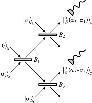
Figure 1: The beamsplitter setup designed for an unambiguous identification of coherent states.

Further, we will consider the UI of coherent states appearing with equal prior probabilities. In this case the optimal choice of transmittivities for our three beamsplitter setup is $T_{1}=1/2$, $T_{2}=2/3$, $T_{3}=1/3$. As a result we obtain that the probability of an unambiguous identification (39) reads

$$P_{bs}(|\alpha_{1}\rangle,|\alpha_{2}\rangle)=1-e^{-\frac{1}{3}|\alpha_{1}-\alpha_{2}|^{2}}\,.$$ (41)

IV.3 Swap-like UI design for coherent states

In this section we will propose different unambiguous identification measurement for coherent states. This approach will be essentially the same as in the construction of the swap-based UI measurement for qudits, i.e. also motivated by the state-comparison problem. The difference is that instead of considering all states we will be restricted to coherent states only, i.e. the role of an antisymmetric subspace is played by the projector ${\openone}-\sum^{\infty}_{N=0}|\chi_{N}\rangle\langle\chi_{N}|)_{AC}$, which was crucial for the optimal state comparison of coherent states (28) discussed in Sec. IV.A. Like before the conclusive POVM elements $E_{j}^{sbf}$ ignore the identified mode and conclusively compare the states in the other two modes, i.e. reading that the states of these two modes are different. Such a POVM has the following structure

$${\rm E}^{sbf}_{1} = c_{1}{\openone}_{B}\otimes({\openone}-\sum^{\infty}_{N=0}|\chi_{N}\rangle\langle\chi_{N}|)_{AC}\,;$$

$${\rm E}^{sbf}_{2} = c_{2}{\openone}_{C}\otimes({\openone}-\sum^{\infty}_{N=0}|\chi_{N}\rangle\langle\chi_{N}|)_{AB}\,;$$

$${\rm E}^{sbf}_{0} = {\openone}-{\rm E}^{sbf}_{1}-{\rm E}^{sbf}_{2}\,.$$ (42)

Let us fix the parameters $c_{1}$, $c_{2}$ and calculate $P_{sbf}(|\alpha_{1}\rangle,|\alpha_{2}\rangle)$ for this UI measurement. Using the identity $\sum^{\infty}_{N=0}|\chi_{N}\rangle\langle\chi_{N}|=\frac{2}{\pi}\int_{\mathbb{C}}|\gamma\rangle\langle\gamma|\otimes|\gamma\rangle\langle\gamma|d\gamma$ [see Eq. (26)] we obtain

$$P_{sbf}(|\alpha_{1}\rangle,|\alpha_{2}\rangle) = (\eta_{1}c_{1}+\eta_{2}c_{2})$$

$$\times (1-\frac{2}{\pi}\int_{\mathbb{C}}|\langle{\alpha_{1}}|\gamma\rangle|^{2}|\langle{\alpha_{2}}|\gamma\rangle|^{2}d\gamma)\,.$$

Taking into account that $|\langle{\alpha}|\gamma\rangle|^{2}=e^{-|\alpha-\gamma|^{2}}$ and the rectangular identity $|a|^{2}+|b|^{2}=\frac{1}{2}(|a+b|^{2}+|a-b|^{2})$ we can express the integral $I=\int_{\mathbb{C}}|\langle{\alpha_{1}}|\gamma\rangle|^{2}|\langle{\alpha_{2}}|\gamma\rangle|^{2}d\gamma$ as follows

$$I = e^{-\frac{1}{2}|\alpha_{1}-\alpha_{2}|^{2}}\int_{\mathbb{C}}e^{-\frac{1}{2}|\alpha_{1}+\alpha_{2}-2\gamma|^{2}}d\gamma$$ (44)

$$= e^{-\frac{1}{2}|\alpha_{1}-\alpha_{2}|^{2}}\int_{\mathbb{C}}e^{-2|\gamma|^{2}}d\gamma=\frac{\pi}{2}e^{-\frac{1}{2}|\alpha_{1}-\alpha_{2}|^{2}}\,.$$

Combining Eqs. (IV.3) and (44) the unambiguous identification probability reads

$$P_{sbf}(|\alpha_{1}\rangle,|\alpha_{2}\rangle)=(\eta_{1}c_{1}+\eta_{2}c_{2})(1-e^{-\frac{1}{2}|\alpha_{1}-\alpha_{2}|^{2}})\,.$$ (45)

The positivity of the POVM elements ${\rm E}^{sbf}_{1}$, ${\rm E}^{sbf}_{2}$ is guaranteed by setting $c_{1}$, $c_{2}$ to be nonnegative. The operator ${\rm E}^{sbf}_{0}$ has a block diagonal structure in the basis consisting of number states ordered with respect to the increasing global photon number. Finding the eigenvalues of this matrix is a difficult problem. Nevertheless, the POVM elements $E_{1}^{sbf}$ and $E_{2}^{sbf}$ are proportional to mutually overlapping projectors. Let $|\mu\rangle_{ABC}$ be a vector from supports of both these projectors. For example, $|\mu\rangle$ can be a vector from the totally antisymmetric subspace. Then $\langle\mu|E_{0}^{sbf}|\mu\rangle=1-c_{1}-c_{2}$. Thus, the positivity implies that $c_{1}+c_{2}\leq 1$. For equal prior probabilities $\eta_{1}=\eta_{2}=1/2$ we obtain

$$P_{sbf}(|\alpha_{1}\rangle,|\alpha_{2}\rangle)\leq\frac{1}{2}(1-e^{-\frac{1}{2}|\alpha_{1}-\alpha_{2}|^{2}})\,.$$ (46)

IV.4 Comparison of UI measurements for coherent states

In the previous sections we have discussed four different UI measurements that can be used to identify coherent states:
i) the swap-based measurement,
ii) the optimal measurement,
iii) the swap-like measurement,
iv) the beamsplitter setup.

The first two schemes unambiguously identify arbitrary states of qudits in arbitrary dimensions. The remaining two are designed to identify only coherent states. Although the comparison is usually understood in terms of average probabilities, we will adopt a different comparison method evaluating the performance directly in terms of probabilities $P(|\alpha_{1}\rangle,|\alpha_{2}\rangle)$ for all pairs of states. It turns out that for all the measurements these probabilities depend only on a scalar product of the states under consideration.

As we mentioned at the beginning of this section qudit POVM elements ${\rm E}^{sb}_{j}$ and ${\rm E}^{opt}_{j}$ in the large-$d$ limit define also POVM elements in ${\cal H}_{\infty}$. For simplicity we use the same notation for these operators. These two UI strategies are universal, so they work for any pure states from ${\cal H}_{\infty}$. If applied on coherent states the corresponding probabilities are given by Eqs. (15) and (20)

$$P_{sb}(|\alpha_{1}\rangle,|\alpha_{2}\rangle)=\frac{1}{4}(1-|\langle{\alpha_{1}}|\alpha_{2}\rangle|^{2})=\frac{1}{4}(1-e^{-|\alpha_{1}-\alpha_{2}|^{2}})\,;$$

$$P_{opt}(|\alpha_{1}\rangle,|\alpha_{2}\rangle)=\frac{1}{3}(1-|\langle{\alpha_{1}}|\alpha_{2}\rangle|^{2})=\frac{1}{3}(1-e^{-|\alpha_{1}-\alpha_{2}|^{2}})\,.$$

In what follows we will compare $P_{sb}(|\alpha_{1}\rangle,|\alpha_{2}\rangle)$, $P_{opt}(|\alpha_{1}\rangle,|\alpha_{2}\rangle)$, and $P_{bs}(|\alpha_{1}\rangle,|\alpha_{2}\rangle)$, $P_{sbf}(|\alpha_{1}\rangle,|\alpha_{2}\rangle)$ which are probabilities of the identification in the UI strategies designed especially for coherent states [see Eqs. (41) and (46)]. The following inequalities hold for arbitrary coherent states $|\alpha_{1}\rangle$ and $|\alpha_{2}\rangle$

$$P_{sb}\leq P_{sbf}\leq P_{bs}\,;\quad P_{opt}\leq P_{bs}\,.$$ (47)

Hence the same relations hold between the measurements also on average. They can all be derived in the same way. Let us define $x=e^{-|\alpha_{1}-\alpha_{2}|^{2}}$ ($x\in[0,1]$) and $\partial_{x}=\frac{\partial}{\partial x}$. All the probabilities are zero for $\alpha_{1}=\alpha_{2}$ ($x=1$) as they should, because in such case reference states coincide. The validity of these inequalities can be proved by showing the reversed inequalities for the first derivatives of probabilities (47) with respect to $x$, i.e.

$$\partial_{x}P_{sb}\geq\partial_{x}P_{sbf}\geq\partial_{x}P_{bs}\,;\quad\partial_{x}P_{opt}\geq\partial_{x}P_{bs}$$

$$\Leftrightarrow$$

$$-\frac{1}{4}\geq-\frac{1}{2x^{\frac{1}{2}}}\geq-\frac{1}{3x^{\frac{2}{3}}}\,;\quad-\frac{1}{3}\geq-\frac{1}{3x^{\frac{2}{3}}}\,.$$

The second row of inequalities obviously holds in the interval $x\in[0,1]$, so the inequalities (47) are proved. More quantitative insight is given in Fig.(2) showing the dependence of the probability of identification for the considered UI measurements on the value of $|\alpha_{1}-\alpha_{2}|$.

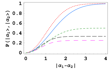
Figure 2: (Color online) The probability of identification $P(|\alpha_{1}\rangle,|\alpha_{2}\rangle)$ as a function of the scalar product (given by $|\alpha_{1}-\alpha_{2}|$) for four UI strategies applied on coherent states $|\alpha_{1}\rangle$, $|\alpha_{2}\rangle$. Starting from the bottom the two lowest lines correspond to universal UI measurements (the swap-based is in magenta (lowest line) and the optimal strategy is in black, respectively). The next two lines are associated with the UI measurements designed for coherent states (the swap-like measurement is in green while the and the three beamsplitters setup is in solid blue, respectively). The top (red) curve corresponds to the optimal discrimination probability among two known states.

As a result we can conclude that the beamsplitter setup designed for an unambiguous identification of coherent states performs better than other devices including the optimal universal UI measurement. Another remarkable feature is that the beamsplitter setup attains $P_{bs}(|\alpha_{1}\rangle,|\alpha_{2}\rangle)=1$ for large values of $|\alpha_{1}-\alpha_{2}|$, i.e. in the limit when two coherent states are orthogonal.

IV.5 Unambiguous identification of $N$ reference states: A quantum database

Now let us consider the problem of unambiguously identification among $N$ coherent states $|\alpha_{1}\rangle,\dots,|\alpha_{N}\rangle$. Our aim is to modify the proposed beamsplitter scheme to address this slightly more general problem. In accordance with the case $N=2$ we will firstly use a beamsplitter array to distribute (to “copy”) the unknown state $|\alpha_{?}\rangle$ onto $N-1$ ancillary modes (which are initially set to the vacuum). After this redistribution of the information we will simultaneously implement $N$-fold state comparison to unambiguously identify the unknown state.

The quantum state distribution can be done with $N-1$ beamsplitters $B_{j}$ (described by parameters $R_{j},T_{j}$) acting on the $j$-th ancillary mode and the mode of an unknown state. The beasmplitters are applied sequentially splitting the unknown state into $N$ modes (see Fig. 3) so that each of them end up in the state $|\frac{1}{\sqrt{N}}{\rm\alpha_{?}}\rangle$. After a little algebra one can derive the following values for reflectivities and transmittivities of the $j$-th beamsplitter

$$T_{j} = \frac{N-j}{N-j+1}\,;$$

$$R_{j} = \frac{1}{N-j+1}\,.$$ (48)

Altogether these beamsplitters will implement the transformation

$$|0\rangle^{\otimes N-1}\otimes|{\rm\alpha_{?}}\rangle\mapsto|\frac{1}{\sqrt{N}}{\rm\alpha_{?}}\rangle^{\otimes N}\,.$$ (49)

After this transformation is completed we will simultaneously apply $N$ beamsplitters performing the quantum state comparison of states $|\frac{1}{\sqrt{N}}\alpha_{?}\rangle$ and $|\alpha_{j}\rangle$. Let us denote by $C_{j}$ the beamsplitter comparing the unknown state with the state of the $j$-th mode. Each of them performs the following transformation

$$\begin{array}[]{rcl}|\frac{1}{\sqrt{N}}{\rm\alpha_{?}},\alpha_{k}\rangle&\to&|\sqrt{\frac{T^{c}_{k}}{N}}{\rm\alpha_{?}}+\sqrt{R^{c}_{k}}\alpha_{k},-\sqrt{\frac{R^{c}_{k}}{N}}{\rm\alpha_{?}}+\sqrt{T^{c}_{k}}\alpha_{k}\rangle\\ &\to&|\sqrt{\frac{1}{N(N+1)}}({\rm\alpha_{?}}+N\alpha_{k}),\frac{1}{\sqrt{N+1}}(\alpha_{k}-{\rm\alpha_{?}})\rangle\,,\end{array}$$

where we used $R^{c}_{k}=\frac{N}{N+1},T^{c}_{k}=\frac{1}{N+1}$ and the notation $|\alpha,\beta\rangle$ for $|\alpha\rangle\otimes|\beta\rangle$. As before the photodetectors monitor the photon number only in the modes originally in states $|\alpha_{j}\rangle$ that at the output are in the state

$$[\otimes^{N-1}_{j=1}|\frac{1}{\sqrt{N+1}}(\alpha_{?}-\alpha_{j})\rangle]\otimes|\frac{1}{\sqrt{N+1}}(\alpha_{N}-\alpha_{?})\rangle\,.$$ (50)

Hence if $|\alpha_{?}\rangle=|\alpha_{k}\rangle$ the $k$-th mode is in the vacuum state and all other modes are excited (i.e., populated by photons). Therefore if all photodetectors except a single one click then we can unambiguously conclude that the unknown state matches with the initial state of the mode corresponding to the detector which did not fire. For all other combination of outcomes the result is inconclusive. This implies that the probability of unambiguous identification for the reference states $|\alpha_{1}\rangle,\ldots,|\alpha_{N}\rangle$ is equal to

$$P(|\alpha_{1}\rangle,\ldots,|\alpha_{N}\rangle)=\sum^{N}_{j=1}\eta_{j}\prod^{N}_{k\neq j}(1-e^{-\frac{1}{\sqrt{N-1}}|\alpha_{k}-\alpha_{j}|^{2}})\,.$$ (51)

If we set $\eta_{j}=\frac{1}{N}$ (for all $j$) and $\alpha_{k}=\alpha e^{\frac{2\pi i}{N}k}$ then the probability can be simplified to

$$P(|\alpha_{1}\rangle,\ldots,|\alpha_{N}\rangle)=\prod^{N-1}_{k=1}\left[1-e^{-\frac{2\alpha^{2}}{\sqrt{N-1}}(1-\cos(\frac{2\pi}{N}k))}\right]\,.$$ (52)

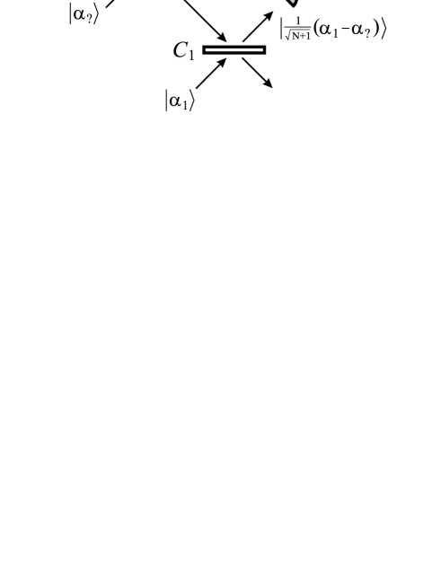
Figure 3: Unambiguous identification measurement setup identifying among $N$ coherent states.

Concluding this section we note that the unambiguous discrimination among $N$ unknown states described above can be considered as a search in a quantum database composed of $N$ elements, i.e. $N$ different though unknown coherent states $|\alpha_{j}\rangle$ that are encoded into $N$ modes of an electromagnetic field. We point out that we have only a single copy of each of the states $|\alpha_{j}\rangle$ so one can not acquire a complete classical knowledge about the state. This set of $N$ states corresponds to a quantum database. In addition we have the $(N+1)$-st mode of the light field in the state $|\alpha_{?}\rangle$. The search of the database corresponds to the task of matching of two modes such that $|\alpha_{?}\rangle=|\alpha_{j}\rangle$. So we can say that the two modes are in the same state without knowing what the state actually is.

V Conclusion

In this paper we have addressed the problem of an unambiguous identification of unknown coherent states. We have explicitly designed two UI measurements taking into account the a priori knowledge about a particular family of states and compare these measurements with the universal unambiguous identification, i.e. the UI measurements (either the swap-based or the optimal one) that can be applied for all states. Our main goal was to design a simple experimental setup consisting of three beamsplitters (see Fig.1) that performs best. Finally, we have generalized the problem and proposed the measurement unambiguously identifying among $N$ coherent state.

The beamsplitter setup was motivated by an intuitive reduction of the unambiguous identification problem into specific “cloning” task and an unambiguous state comparison. We have proved that the state comparison originally proposed in andersson is indeed the optimal one (this was implicitly conjectured in Ref. andersson but was not proved). It is interesting to compare UI measurements described in this paper with an UI measurement given as a mixture of two optimal unambiguous comparison measurements, i.e. $\overline{E}_{1}=qI_{B}\otimes F^{\rm dif}_{AC}$, $\overline{E}_{2}=qI_{C}\otimes F^{\rm dif}_{AB}$, $\overline{E}_{0}=I-\overline{E}_{1}-\overline{E}_{2}$. Let us consider the UI problem for pure states belonging to a set $S$ such that $\int_{S}|\psi\rangle\langle\psi|\otimes|\psi\rangle\langle\psi|d\psi=\Pi(S)$ is a projector. Under such assumption the conclusive result for an optimal unambiguous comparison of states from $S$ is associated with the positive operator $F^{\rm dif}=I-\Pi(S)$. If $S=S_{d}$ is the set of all pure states of $d$-dimensional system then $F^{\rm dif}=I-\Pi(S_{d})=I-\Pi_{\rm sym}={\rm ASym}$. Hence, the corresponding POVM consists of operators $\overline{E}_{1}=\frac{1}{2}I_{B}\otimes{\rm ASym}_{AC}$, $\overline{E}_{2}=\frac{1}{2}I_{C}\otimes{\rm ASym}_{AB}$, i.e. (for $d>2$) it is exactly the SWAP-based UI measurement as specified in Eq.(16). Similarly for coherent states we have $F^{\rm dif}=I-\Pi(S_{\rm coh})=I-\frac{2}{\pi}\Delta$ (see Eq.(26)) and the mixing of optimal unambiguous comparison strategies results in the same POVM as in Eq.(42). Based on our results we can say that although for purposes of the state comparison problem the operator ${\openone}-\Pi({\cal S})$ is the optimal solution, the resulting UI measurement based on mixing of such optimal unambiguous comparison strategies is not the optimal one.

The proposed beamsplitters setup (see Fig.1) for unambiguous state identification can be compared with the measurement proposed in Ref. banaszek discriminating optimally among two known coherent states. Both of them consists of three beamsplitters, but arranged differently. An interesting observation is that the differences between the probabilities are not very large (see Fig.2) and even more surprising is the fact that two unknown nearly orthogonal coherent states can be identified almost perfectly. For the universal optimal UI measurement (see Fig.2) there is a significant gap between the probabilities for state discrimination and state identification.

The proposal of unambiguous identification of coherent states is extended for an arbitrary number $N$ of reference states. We proposed an experimental setup consisting of $2N-1$ beamsplitters for unambiguous identification among $N$ unknown coherent states. This setup can be considered as a search in a quantum database. The elements of the database are unknown coherent states encoded in different modes of an electromagnetic field. The task is to specify the two modes that are excited in the same, though unknown, coherent state. The analysis of this aspect of unambiguous identification problem is beyond the scope of this paper and details will be presented elsewhere.

Appendix A Eigenvalues of $E_{0}^{sb}$

The operator ${\rm E}_{0}^{sb}$ is defined in Eq.(12). As we have already mentioned in Section IIIA this operator is block diagonal and consists of three types of blocks.

1. Trivial $\langle iii|{\rm E}_{0}^{sb}|iii\rangle=1$.

2. $3\times 3$ matrix $\langle\sigma_{1}(iij)|{\rm E}_{0}^{sb}|\sigma_{2}(iij)\rangle$:

$$Q_{3}=\begin{pmatrix}&iij&iji&jii\\ iij&1-c_{1}/2&0&c_{1}/2\\ iji&0&1-c_{2}/2&c_{2}/2\\ jii&c_{1}/2&c_{2}/2&1-c_{1}/2-c_{2}/2\end{pmatrix}$$ (53)

with eigenvalues

$$\lambda^{(3)}_{1} = 1\,;$$ (54)

$$\lambda^{(3)}_{2,3} = \frac{2-c_{1}-c_{2}\pm\sqrt{c_{1}^{2}-c_{1}c_{2}+c_{2}^{2}}}{2}$$

3. $6\times 6$ matrix $\langle\sigma_{1}(ijk)|{\rm E}_{0}^{sb}|\sigma_{2}(ijk)\rangle$:

$$Q_{6}=\begin{pmatrix}&ijk&kji&jki&ikj&kij&jik\\ ijk&X&c_{1}/2&0&0&0&c_{2}/2\\ kji&c_{1}/2&X&c_{2}/2&0&0&0\\ jki&0&c_{2}/2&X&c_{1}/2&0&0\\ ikj&0&0&c_{1}/2&X&c_{2}/2&0\\ kij&0&0&0&c_{2}/2&X&c_{1}/2\\ jik&c_{2}/2&0&0&0&c_{1}/2&X\end{pmatrix}\,,$$ (55)

where $X=1-\frac{c_{1}}{2}-\frac{c_{2}}{2}$. The corresponding eigenvalues read

$$\begin{array}[]{l}\lambda^{(6)}_{1}=1\\ \lambda^{(6)}_{2}=1-c_{1}-c_{2}\\ \lambda^{(6)}_{3,4}=\frac{2-c_{1}-c_{2}+\sqrt{c_{1}^{2}-c_{1}c_{2}+c_{2}^{2}}}{2}\\ \lambda^{(6)}_{5,6}=\frac{2-c_{1}-c_{2}-\sqrt{c_{1}^{2}-c_{1}c_{2}+c_{2}^{2}}}{2}\,.\end{array}$$ (56)

For qubits we have $2^{3}$-dimensional Hilbert space and ${\rm E}_{0}^{sb}$ is represented by $8\times 8$ matrix with two $3\times 3$ blocks and two $1\times 1$ blocks. So for qubits the sufficient condition for positivity of ${\rm E}_{0}^{sb}$ reads

$$2-c_{1}-c_{2}\pm\sqrt{c_{1}^{2}-c_{1}c_{2}+c_{2}^{2}}\geq 0$$

For qudits, $d>2$, at least one $6\times 6$ block appears in the matrix of ${\rm E}_{0}^{sb}$. The eigenvalues of the $6\times 6$ block satisfy the following inequality:

$$\lambda^{(6)}_{1}\geq\lambda^{(6)}_{3,4}\geq\lambda^{(6)}_{5,6}\geq\lambda^{(6)}_{2},$$

so the sufficient condition for positivity of ${\rm E}_{0}^{sb}$ when $d>2$ is $\lambda^{(6)}_{2}=1-c_{1}-c_{2}\geq 0$.

Appendix B Calculation of $\Delta$

In this appendix we will explicitly evaluate the operator

$$\Delta = \int_{\mathbb{C}}|\alpha\rangle_{X}\otimes|\alpha\rangle_{Y}{}_{X}\langle\alpha|\otimes{}_{Y}\langle\alpha|\quad d\alpha\,.$$ (57)

First expand the coherent state $|\alpha\rangle$ in the number basis and use the polar parametrization of the complex plane

$$|\alpha\rangle=e^{-\frac{|\alpha|^{2}}{2}}\sum^{\infty}_{k=0}\frac{\alpha^{k}}{\sqrt{k!}}|k\rangle,\quad\alpha=re^{i\phi},\quad d\alpha=rdrd\phi$$

in order to write

$$\Delta = \int_{\mathbb{C}}e^{-2|\alpha|^{2}}\sum^{\infty}_{k,l,m,n=0}\frac{\alpha^{k+l}(\alpha^{\ast})^{m+n}}{\sqrt{k!l!m!n!}}|k\rangle\langle m|\otimes|l\rangle\langle n|d\alpha$$

$$= \left(\sum^{\infty}_{k,l,m,n=0}\frac{1}{\sqrt{k!l!m!n!}}\int^{\infty}_{0}e^{-2r^{2}}r^{k+l+m+n+1}dr\right)$$

$$\times \int^{2\pi}_{0}e^{i\phi(k+l-m-n)}d\phi|kl\rangle\langle mn|\,.$$

The integration over $\phi$ yields $2\pi\delta_{k+l,m+n}$ and the integration over $r$ after a simple substitution and usage of $\delta_{k+l,m+n}$ leads to $\Gamma(k+l+1)/2^{k+l}$. Using the identity $\Gamma(k+l+1)=\sqrt{(k+l)!}\sqrt{(m+n)!}$ we obtain

$$\Delta = \frac{\pi}{2}\sum^{\infty}_{k,l,m,n=0}\frac{\sqrt{\binom{m+n}{m}}\sqrt{\binom{k+l}{k}}}{2^{\frac{k+l}{2}}2^{\frac{m+n}{2}}}\delta_{k+l,m+n}|kl\rangle\langle mn|\,.$$

Defining a new summation index $N=m+n=k+l$ and using $\delta_{k+l,m+n}$ we eliminate one sum to obtain

$$\Delta = \frac{\pi}{2}\sum^{\infty}_{N=0}\sum^{N}_{k,m=0}\frac{\sqrt{\binom{N}{k}}\sqrt{\binom{N}{m}}}{2^{\frac{N}{2}}2^{\frac{N}{2}}}|k\rangle|N-k\rangle\langle m|\langle N-m|$$ (58)

$$= \frac{\pi}{2}\sum^{\infty}_{N=0}(|\chi_{N}\rangle\langle\chi_{N}|)_{XY},$$

where we defined mutually orthogonal vectors

$$|\chi_{N}\rangle=2^{-\frac{N}{2}}\sum^{N}_{k=0}\sqrt{\binom{N}{k}}|k\rangle_{X}\otimes|N-k\rangle_{Y}\,,$$ (59)

i.e. $\langle{\chi_{N}}|\chi_{M}\rangle=\delta_{N,M}$.

Appendix C Calculation of $U^{\dagger}|N\rangle_{X}\otimes|0\rangle_{Y}$

The action of the 50/50 beamsplitter unitary transformation $U$ on the creation operators $a^{\dagger}$, $b^{\dagger}$ of modes X and Y is given by

$$U^{\dagger}a^{\dagger}U = \frac{1}{\sqrt{2}}(a^{\dagger}+b^{\dagger})$$ (60)

$$U^{\dagger}b^{\dagger}U = \frac{1}{\sqrt{2}}(-a^{\dagger}+b^{\dagger})$$ (61)

Let us express the number (Fock) state via the creation operators acting on the vacuum, i.e. $|N\rangle_{X}=(a^{\dagger})^{N}/\sqrt{N!}|0\rangle_{X}$. The vacuum is unaffected by both $U$ and $U^{\dagger}$. Having all this in mind we can calculate the state $|\chi_{N}\rangle=U^{\dagger}|N\rangle_{X}|0\rangle_{Y}$

$$|\chi_{N}\rangle=\frac{1}{\sqrt{N!}}(U^{\dagger}a^{\dagger}U)^{N}|0\rangle|0\rangle$$

$$=\frac{1}{2^{\frac{N}{2}}\sqrt{N!}}(a^{\dagger}+b^{\dagger})^{N}|0\rangle|0\rangle$$

$$=\frac{1}{2^{\frac{N}{2}}}\sum^{N}_{k=0}\sqrt{\frac{k!(N-k)!)}{N!}}\binom{N}{k}\frac{(a^{\dagger})^{k}}{\sqrt{k!}}\frac{(b^{\dagger})^{N-k}}{\sqrt{(N-k)!}}|0\rangle|0\rangle$$

$$=\frac{1}{2^{\frac{N}{2}}}\sum^{N}_{k=0}\sqrt{\binom{N}{k}}|k\rangle|N-k\rangle.$$

References

• (1) C.W. Helstrom, Quantum Detection and Estimation Theory (Academic Press, New York, 1976).
• (2) I.D. Ivanovic, How to differentiate between non-orthogonal states, Phys. Lett. A 123, 257 (1987).
• (3) D. Dieks, Overlap and distinguishability of quantum states, Phys. Lett. A 126, 303 (1988).
• (4) A. Peres, How to differentiate between non-orthogonal states, Phys. Lett. A 128, 19 (1988).
• (5) G. Jaeger and A. Shimony, Optimal distinction between two non-orthogonal quantum states, Phys. Lett. A 197, 83 (1995).
• (6) K. Banaszek, Quantum homodyne tomography with a priori constraints, Phys. Lett. A 253, 12 (1999).
• (7) S.M. Barnett, A. Chefles, and I. Jex, Comparison of two unknown pure quantum states, Phys. Lett. A 307, 189 (2003).
• (8) I.Jex, E.Andersson, A.Chefles, Comparing the states of many quantum systems, Journal of Modern Optics 51, 505 (2004).
• (9) E. Andersson, M. Curty, and I. Jex, Experimentally realizable quantum comparison of coherent states and its applications, Phys. Rev. A 74, 022304 (2006).
• (10) J. Bergou and M. Hillery, Universal programmable quantum state discriminator that is optimal for unambiguously distinguishing between unknown states, Phys. Rev. Lett. 94, 160501 (2005).
• (11) S. Massar and S. Popescu, Optimal extraction of information from finite quantum ensembles, Phys. Rev. Lett. 74, 1259 (1995).
• (12) R. Derka, V. Bužek, and A. Ekert, Universal algorithm for optimal state estimation from finite ensembles. Phys. Rev. Lett. 80, 1571 (1998).
• (13) M. Nielsen and I. Chuang, Programmable quantum gate arrays, Phys. Rev. Lett. 79, 321 (1997).
• (14) M. Hillery, V. Bužek, and M. Ziman, Probabilistic implementation of universal quantum processors, Phys. Rev. A 65, 022301 (2002).
• (15) M. Dušek and V. Bužek, Quantum multimeters: A programmable state discriminator, Phys. Rev. A 66, 022112 (2002).
• (16) V. Bužek, M. Hillery, M. Ziman, and M. Roško, Programmable quantum processors, Quantum Information Processing 5, 303 – 420 (2006).
• (17) M. Roško, V. Bužek, P.R. Chouha, and M. Hillery, Generalized measurements via programmable quantum processor, Phys. Rev. A 68, 062302 (2003).
• (18) J. Bergou, V. Bužek, E. Feldman, U. Herzog, and Mark Hillery, Programmable quantum-state discriminators with simple programs, Phys. Rev. A 73, 062334 (2006).
• (19) A. Hayashi, M. Horibe, and T. Hashimoto, Unambiguous pure-state identification without classical knowledge, Phys. Rev. A 73, 012328 (2006).
• (20) C. Zhang and M. Ying, Universal programmable devices for unambiguous discrimination, arXiv:quant-ph/0606189 (2006).
• (21) K. Zyckowski and I. Bengtsson, Geometry of Quantum States (Cambridge University Press, 2006).
• (22) V. Bužek and M. Hillery, Quantum copying: Beyond the noncloning theorem, Phys. Rev. A 54, 1844 (1996).
• (23) S.L. Braunstein, N.J. Cerf, S. Iblisdir, P. van Loock, and S. Massar, Optimal cloning of coherent states with linear amplifier and beam splitters, Phys. Rev. Lett 86, 4938 (2001).