Determinant solution for the Totally Asymmetric Exclusion Process with parallel update II. Ring geometry.

Abstract

Using the Bethe ansatz we obtain the determinant expression for the time dependent transition probabilities in the totally asymmetric exclusion process with parallel update on a ring. Developing a method of summation over the roots of Bethe equations based on the multidimensional analogue of the Cauchy residue theorem, we construct the resolution of the identity operator, which allows us to calculate the matrix elements of the evolution operator and its powers. Representation of results in the form of an infinite series elucidates connection to other results obtained for the ring geometry. As a byproduct we also obtain the generating function of the joint probability distribution of particle configurations and the total distance traveled by the particles.

1 Introduction

The present paper can be viewed as a continuation of the paper [1], where the transition probabilities for the totally asymmetric simple exclusion process (TASEP) with parallel update have been obtained for the 1D infinite lattice, generalizing well-known result of Schütz [2] for the continuous time TASEP. The analytic method, developed in the first half of that paper, was based on the use of Bethe eigenvectors of the evolution operator obtained in [3]. The problem was to find a continuous spectrum, i.e. the integration measure, which would allow one to construct the solutions of the master equation out of the Bethe eigenvectors, and in particular would give a resolution of the identity operator in the integral form. The proof of the formula for the resolution of the identity operator, was the main technical result of the paper which yielded the final determinant formula for the transition probability.

A peculiarity of the finite ring is that the spectrum becomes discrete due to the periodic boundary conditions, being defined by the system of the algebraic Bethe equations (BE). These equations usually cannot be solved exactly. Most attempts to extract any information from them are related to the thermodynamic limit, where they can be reinterpreted in terms of a single integral equation. For the finite lattices, not only the exact form of the spectrum but even the issue of its completeness are far from being well understood for most of the integrable models.

Fortunately, for the TASEP the situation is a bit better due to a very special factorization property possessed by the BE. This property was observed already in one of the first works on the continuous time TASEP by Gwa and Spohn [4], where it was used to get the asymptotical behaviour of the spectral gap. One of the most impressive results exploiting the special structure of the BE in TASEP was the exact derivation of the largest eigenvalue of the equation for the generating function of the integrated particle current, due to Derrida and Lebowitz [5]. Using the Cauchy residue theorem, they managed to evaluate explicitly the sum over roots of the BE for the particular solution corresponding to the groundstate of the evolution operator. Recently, some peculiar details of the spectrum structure for the continuous time TASEP have been also studied in [6].

The solution of the Cauchy problem, i.e. finding the solution, given the initial conditions, for the master equation for the TASEP on the ring in continuous time, and also with backward ordered update, has been recently proposed by one of the authors [7]. To our knowledge, this is still the only example of full solution to the Cauchy problem for an integrable model that cannot be reduced to free fermions. The method of the solution is based on a geometric approach to the Bethe ansatz (BA), which treats trajectories of the interacting particles as free, noninteracting, but supplied with the additional statistical weights in such a way that the interaction is taken into account. The idea of the solution on a ring was to represent it as an infinite line with periodic patterns of synchronously moving interacting particles. As in the geometric formulation one works only with the ensembles of particle trajectories of a finite length, the issues related to the structure of the eigenspace of the evolution operator can be by-passed. Motivated by the geometric solution, its analytic counterpart called the detailed BA has been also proposed [8]. Being defined on the infinite lattice, the detailed BA has a form of the infinite formal sum, and can be considered as a generating function of particle trajectories. As a result, the problem becomes infinite lattice-like and one can again use integration over the continuum to reconstruct the transition probabilities. The mathematical meaning of the term-by-term integration of the infinite formal series was not yet well understood,  and, as we will see below, it is just equivalent to summation over the discrete spectrum given by the BE.

The geometric method was applied to the TASEP with parallel update on the infinite lattice in the second half of our first paper [1]. Its generalization to the ring geometry follows in line with the continuous time version and as such is straightforward. Therefore, the aim of this paper is not only to obtain the solution of the Cauchy problem for the TASEP with parallel update, but also to establish a bridge between existing solutions on a ring and the standard BA techniques. Namely, we show that the idea of Derrida and Lebowitz exploiting the Cauchy residue theorem to obtain the roots of the BE corresponding to the groundstate solution can be developed much further and used to perform an exact summation over the whole spectrum of solutions. In such a way we obtain the integral representation for the resolution of the identity operator and, as a consequence, for the solution of the Cauchy problem for the master equation as well. Then we show that the expression under the integral can be expanded into a uniformly converging power series, equivalent to the detailed BA, which being integrated term by term yields finally the multiple infinite sums coming from the geometric solution and from the detailed BA.

The paper is organized as follows. In section II, we formulate the dynamical rules of the model and announce the final result. In section III, we describe the BA for the infinite lattice and give the BE for the ring. In section IV, we discuss the details of the analytic structure of the BE solutions. In section V we develop a technique of evaluation of sums over the Bethe roots. In section VI, we prove a formula for the resolution of the identity operator and obtain a formula for transition probabilities in the form of infinite sums. Then, to show that the sums are actually finite, we estimate the number of nonzero terms they contain. In the last section VII, we discuss the results obtained and subsequent perspectives.

2 Formulation of the model and results

We consider $P$ particles on the 1D ring consisting of $L$ sites. The notation

$$\rho=P/L$$ (1)

is used for the density of particles. The model has totally asymmetric dynamics, i.e. all particles jump only in one direction, which we refer to as forward. At each step of discrete time $t$, a particle from each occupied site,

i

takes one step forward with probability $v$

or

ii

stays with probability $(1-v)$,

provided that the target site is vacant. When the next site is occupied,

iii

a particle stays with probability $1$.

All sites are updated simultaneously. We define a configuration $X$ of particles by the set of their coordinates $X=\left\{x_{1},x_{2},\ldots,x_{P}\right\}$, written in strictly increasing order,

$$x_{1}<x_{2}<\cdots<x_{P}.$$ (2)

The finite ring geometry implies also that the coordinates are confined to the values from $1$ to $L$.

$$x_{1}\geq 1,x_{P}\leq L$$ (3)

The probability $P_{t}(X)$ for the system to be in a configuration $X$ at time $t$ obeys the Markov equation

$$P_{t+1}(X)=\sum_{\left\{X^{\prime}\right\}}T(X,X^{\prime})P_{t}(X^{\prime}),$$ (4)

where $T(X,X^{\prime})$ is the probability of the transition from $X^{\prime}$ to $X$ for one time step. The transition probability $T(X,X^{\prime})$ defined by the above dynamical rules is a product of factors, each corresponding to a particular cluster of particles in the initial configuration $X^{\prime}$. The word ”cluster” refers to a group of particles, which has no empty sites between occupied sites and two empty sites at the ends. The value of these factors is either $v$ or $(1-v)$ depending on whether or not the first particle of a given cluster jumps during the transition from $X^{\prime}$ to $X.$

$$T(X,X^{\prime})=\prod\limits_{i=1}^{\mathcal{N}_{c}\left(X^{\prime}\right)}\left(1-v\right)^{1-m_{i}}v^{m_{i}}$$ (5)

Here $m_{i}=0,1$ is the number of particles hopping from $i$-th cluster of $X^{\prime}$, and ${\mathcal{N}_{c}\left(X^{\prime}\right)}$ is the number of clusters in $X^{\prime}$.

It has been shown in [1] that in the case of the infinite lattice, when constraint (3) is omitted, the conditional probability, $P(X;t|X^{0};0)$, for the system to be in a configuration $X=\left\{x_{1},x_{2},\ldots,x_{P}\right\}$ at time $t$, given it was in a configuration $X^{0}=\left\{x_{1}^{0},x_{2}^{0},\ldots,x_{P}^{0}\right\}$ at time $0$, is the following quotient

$$P(X;t|X^{0};0)=\frac{\mathcal{F}_{\infty}\left(X,X^{0},t\right)}{\mathcal{F}_{\infty}\left(X,X,0\right)}\mathbf{.}$$ (6)

The function $\mathcal{F}_{\infty}\left(X,Y,t\right)$ depending on two particle configurations $X=\left\{x_{1},x_{2},\ldots,x_{P}\right\}$ and $Y=\left\{y_{1},y_{2},\ldots,y_{P}\right\}$ and on time $t$ is given by the determinant of $P\times P$ matrix

$$\mathcal{F}_{\infty}\left(X,Y,t\right)=\det\left[f(i-j,x_{i}-y_{j},t)\right]_{1\leq i,j\leq P},$$ (7)

where the matrix elements are defined in terms of a single function $f\left(a,b,t\right)$ expressed via the Gauss hypergeometric functions:

$$~{}f(a,b,t)=\left(1-v\right)^{t}\cases{\begin{array}[]{ll}\left(\frac{v}{v-1}\right)^{b}\frac{(-t-a)_{b}}{b!}\left.{}_{2}F_{1}\right.\left(\begin{array}[]{c}a,-t-a+b\\ b+1\end{array};\frac{v}{v-1}\right)&b>0\\ \frac{\left(a\right)_{-b}}{\left(-b\right)!}\left.{}_{2}F_{1}\right.\left(\begin{array}[]{c}a-b,-t-a\\ -b+1\end{array};\frac{v}{v-1}\right)&b\leq 0\end{array}.}$$ (8)

The notation $\left(a\right)_{n}$ is for the shifted factorial $\left(a\right)_{n}=a(a+1)\cdots\left(a+n-1\right)$.

The aim of the present article is to show that on the ring of size $L$ the same quantity $P(X;t|X^{0};0)$ is also given by similar quotient of two terms, both expressed as a single function $\mathcal{F}_{L}\left(X,Y,t\right)$ of particle configurations $X,Y$ and time $t$,

$$P(X;t|X^{0};0)=\frac{\mathcal{F}_{L}\left(X,X^{0},t\right)}{\mathcal{F}_{L}\left(X,X,0\right)}$$ (9)

with the arguments in the numerator and the denominator taken as in (6). However, for the finite ring, the function $\mathcal{F}_{L}\left(X,Y,t\right)$ is the $P$-tuple sum of determinants

$$\mathcal{F}_{L}\left(X,Y,t\right)=\sum\limits_{n_{1}=-\infty}^{\infty}\cdots\sum\limits_{n_{P}=-\infty}^{\infty}\left(-1\right)^{(P-1)\sum_{i=1}^{P}n_{i}}$$

$$\times\det\left[f\left(i-j+Pn_{i}-\sum\limits_{k=1}^{P}n_{k},x_{i}-y_{j}+n_{i}L,t\right)\right]_{1\leq i,j\leq P},$$ (10)

unlike the single determinant in the case of infinite lattice. The matrix elements of the corresponding matrices are still given in terms of the function $f\left(a,b,t\right)$ defined in (8), but its arguments depend now not only on the matrix indices $i,j$ but also on summation indices $n_{k}$. Below we argue that though formally the sums are infinite, they contain only a finite number of nonzero terms for any finite time $t$. Furthermore, the denominators of (6) and (9) depend only on the number of clusters in the corresponding configuration $X$ being equal to

$$\mathcal{F}_{\infty}\left(X,X,0\right)=\mathcal{F}_{L}\left(X,X,0\right)=\left(1-v\right)^{\mathcal{N}_{c}\left(X\right)-P}$$ (11)

Remark 1

One has to define $\mathcal{N}_{c}\left(X\right)$ in (11) as a function of $X$ separately for the infinite and finite lattices. Indeed, the particles, which occupy the sites $1$ and $L$ on the ring, belong to the same cluster, while on the infinite lattice they do not. Therefore, the value of $\mathcal{N}_{c}(X)$ can be different for these two cases, even though the coordinates of particles formally coincide.

3 Bethe ansatz.

3.1 Infinite lattice.

We first remind the reader of the technique used to deal with the infinite lattice case [1]. Consider $P$ particles on the infinite lattice. The particle configurations are given by $P-$tuples of particle coordinates which are unbounded integers being selected from the set

$$\mathbb{Z}_{<}^{P}\equiv\left\{X\in\mathbb{Z}^{P};x_{1}<x_{2}<\cdots<x_{P}\right\}.$$ (12)

Let us introduce the infinite dimensional vector space $V_{\infty}$ over the field of complex numbers $\mathbb{C}$ given by the linear span of the basis

$$\mathcal{X}_{\infty}=\left\{\left|X\right\rangle:X\in\mathbb{Z}_{<}^{P}\right\},$$ (13)

i.e. the set of the vectors labelled by the particle configurations. In addition one introduces the basis of the dual space $V_{\infty}^{\ast}$, which is the span of the dual basis,

$$\mathcal{X}_{\infty}^{\ast}=\left\{\left\langle X\right|:X\in\mathbb{Z}_{<}^{P}\right\},$$ (14)

with the inner product defined by

$$\left\langle X|X^{\prime}\right\rangle=\delta(X,X^{\prime}).$$ (15)

Below the bases $\mathcal{X}$,$\mathcal{X}^{\ast}$ will be referred to as the configurational left and right bases respectively, unlike the left and right eigenbases of the evolution operator to be considered. The evolution operator $\mathbf{T}$ is defined in terms of the transition probabilities $T(X,X^{\prime})$ defined in (5)

$$\mathbf{T=}\sum_{X\in\mathcal{X}_{\infty},X^{\prime}\in\mathcal{X}_{\infty}^{\ast}}\left|X\right\rangle T(X,X^{\prime})\left\langle X^{\prime}\right|.$$ (16)

The problem under consideration is to find the transition probability $P(X;t|X^{0};0)$ from a configuration $X^{0}$ to $X$ for $t$ steps, which is nothing but the corresponding matrix element of the operator $\mathbf{T}^{t}$

$$P(X;t|X^{0};0)=\left\langle X|\mathbf{T}^{t}|X_{0}\right\rangle.$$

It was shown in [3], [1] that the evolution operator $\mathbf{T}$ has the left and right eigenvectors $\left|B_{Z}\right\rangle$, $\left\langle\overline{B}_{Z}\right|$ parametrized by $P$-tuple complex parameter

$$Z\equiv\left\{z_{1},\ldots,z_{P}\right\}\in\mathbb{C}^{P}.$$

The eigenvectors corresponding to the same value of $Z$ solve the left and right eigenproblems,

$$\mathbf{T}\left|B_{Z}\right\rangle=\Lambda(Z)\left|B_{Z}\right\rangle,\left\langle\overline{B}_{Z}\right|\mathbf{T}=\Lambda(Z)\left\langle\overline{B}_{Z}\right|,$$ (17)

associated with the same eigenvalue

$$\Lambda\left(Z\right)=\left(1+\lambda\right)^{-P}\prod\limits_{i=1}^{P}\left(1+\lambda z_{i}\right),$$ (18)

where we introduce the parameter $\lambda$

$$\lambda=\frac{v}{1-v}.$$ (19)

The projection $\left\langle X|B_{Z}\right\rangle$ of the right eigenvector $\left|B_{Z}\right\rangle$ to the configuration $X$ is given by the Bethe ansatz

$$\left\langle x_{1},\ldots,x_{P}|B_{Z}\right\rangle=W(X)\sum_{\left\{\sigma\right\}}A_{\sigma_{1}\ldots\sigma_{P}}z_{\sigma_{1}}^{-x_{1}}\ldots z_{\sigma_{P}}^{-x_{P}},$$ (20)

supplied with the additional configuration-dependent factor $W(X)$. The latter is proportional to the stationary measure of the configuration $X$ and is defined in terms of the number of clusters $\mathcal{N}_{c}\left(X\right)$ in the configuration $X$

$$W\left(X\right)=\left(1+\lambda\right)^{\mathcal{N}_{c}\left(X\right)-P}.$$ (21)

The amplitudes $A_{\sigma}$, are indexed by the permutations $\sigma=$ $\left\{\sigma_{1},\cdots,\sigma_{P}\right\}$ of the integers $1,\ldots,P$. An elementary transposition of two indices $(ij)$ results in the amplitude $A_{\sigma}$ being multiplied by the scattering factor $-S\left(z_{i},z_{j}\right)$,

$$A_{\ldots ij\ldots}=-S\left(z_{i},z_{j}\right)A_{\ldots ji\ldots},$$ (22)

of the following form

$$S\left(z_{i},z_{j}\right)\equiv\frac{1-1/z_{i}}{1-1/z_{j}}\frac{1+\lambda z_{j}}{1+\lambda z_{i}}.$$ (23)

A remarkable property of the scattering factor $S\left(z_{i},z_{j}\right)$ is that it is a product of two factors, each being dependent only on one of the two parameters $z_{i}$, $z_{j}$. This property allows one to represent the amplitude $A_{\sigma}$ in a simple product form

$$A_{\sigma_{1}\ldots\sigma_{P}}=\left(-1\right)^{\left|\sigma\right|}\prod\limits_{i=1}^{P}\left(\frac{1+\lambda z_{\sigma_{i}}}{1-1/z_{\sigma_{i}}}\right)^{i-\sigma_{i}},$$ (24)

where each multiple depends only on one of the parameters $z_{1},\ldots,z_{P}$. Unlike the right eigenvector, the left one, $\left\langle\overline{B}_{Z}\right|,$ has no factor $W(X)$, while the Bethe part can be obtained from that of (20) by the change $A_{\sigma}\rightarrow A_{\sigma}^{-1}$, $x_{i}\rightarrow-x_{i}$.

$$\left\langle\overline{B}_{Z}|x_{1},\ldots,x_{P}\right\rangle=\sum_{\left\{\sigma\right\}}A_{\sigma_{1}\ldots\sigma_{P}}^{-1}z_{\sigma_{1}}^{x_{1}}\ldots z_{\sigma_{P}}^{x_{P}}.$$ (25)

Then, that the projection of the eigenvectors $\left\langle\overline{B}_{Z}|X\right\rangle$ and $\left\langle X|B_{Z}\right\rangle$ to the basis vectors corresponding to a particular configuration $X$ can be represented in the form of determinants

$$\left\langle X|B_{Z}\right\rangle = W(X)\det\mathbf{B,}$$ (26)

$$\left\langle\overline{B}_{Z}|X\right\rangle = \det\overline{\mathbf{B}},$$ (27)

where the matrix elements $B_{ij}$ and $\overline{B}_{ij}$ are given by

$$B_{ij}=1/\overline{B}_{ij}=\left(\frac{1+\lambda z_{j}}{1-1/z_{j}}\right)^{i-j}z_{j}^{-x_{i}}.$$ (28)

One of the main results of  [1] is the proof of the formula for the resolution of the identity operator,

$$\int\left|B_{Z}\right\rangle\left\langle\overline{B}_{Z}\right|d\mu(Z)=\mathbf{E},$$ (29)

where $\mathbf{E}$ is the identity operator, $d\mu(Z)=\left(P!\right)^{-1}\prod\nolimits_{i=1}^{P}\left(dz_{i}/2\pi\mathrm{i}z_{i}\right)$ is the integration measure, and the integration is performed independently over each $z_{i}$ along the contour $\Gamma^{\infty}$ encircling the points $z=0$ and $z=1$, while the point $z=-1/\lambda$ stays outside (figure 1). Practically the proof was given by the direct evaluation of the integral in the configurational basis,

$$\int\left\langle X^{\prime}|B_{Z}\right\rangle\left\langle\overline{B}_{Z}|X\right\rangle d\mu(Z)=\delta_{X,X^{\prime}}.$$ (30)

Figure 1: Shape of the contour $\Gamma^{\infty}$. It must encircle the points $z=1$ and $z=0$ while the point $z=-1/\lambda$ stays outside.

As soon as the equality (29) is established, one can insert the identity operator into the matrix elements,

$$\left\langle X\right|\mathbf{T}^{t}\left|X^{0}\right\rangle = \int\left\langle X|\mathbf{T}^{t}|B_{Z}\right\rangle\left\langle\overline{B}_{Z}|X^{0}\right\rangle d\mu(Z)$$ (31)

$$= \int\Lambda^{t}\left(Z\right)\left\langle X|B_{Z}\right\rangle\left\langle\overline{B}_{Z}|X^{0}\right\rangle d\mu(Z)$$ (32)

so that the final result (6-8) immediately follows from the explicit form of the eigenvalues and the eigenvectors.

One of the observations made in [1] was that there is no any obvious procedure of choosing a contour and a measure of integration. However, validity of a particular choice can be verified a posteriori by proving the resolution of the identity operator, which is fulfilled by a direct evaluation of l.h.s. of (30). It will be clear below that the form of the contour can be validated directly by considering the infinite lattice as a limiting case of the ring of the size $L$, which grows to infinity. Then, the $Z-$spectrum of the model is obtained as a continuous limit of the discrete spectrum for the finite system.

3.2 The ring.

What does change when one confines the system to the ring of finite length $L$? Apparently, the total number of particle configurations becomes finite. The same must be true for the dimension of vector space $V_{L}$ defined as the span of the basis

$$\mathcal{X}_{L}=\left\{\left|X\right\rangle:X\in\mathbb{Z}_{<,L}^{P}\right\},$$ (33)

where $\mathbb{Z}_{<,L}^{P}$ is the domain for particle coordinates on the ring.

$$\mathbb{Z}_{<,L}^{P}\equiv\left\{X\in\mathbb{Z}^{P};1\leq x_{1}<x_{2}<\cdots<x_{P}\leq L\right\}.$$ (34)

As before, the dual space $V_{L}^{\ast}$ is spanned by the dual basis

$$\mathcal{X}_{L}^{\ast}=\left\{\left\langle X\right|:X\in\mathbb{Z}_{<,L}^{P}\right\},$$ (35)

with the inner product defined by

$$\left\langle X|X^{\prime}\right\rangle=\delta(X,X^{\prime}).$$

Obviously, the dimensions of the spaces are equal to the total number of the basis vectors, which is equal to the number of particle configurations:

$$\dim\left(V_{L}\right)=\dim\left(V_{L}^{\ast}\right)=\left(\begin{array}[]{c}L\\ P\end{array}\right).$$ (36)

The solution of the eigenproblem turns out to be analogous to the infinite lattice case. The only though important difference is that, due to the finite dimension of the vector space, a finite number of independent eigenvectors can exist. Technically this follows from the fact that vectors $\left|B_{Z}\right\rangle$ and $\left\langle\overline{B}_{Z}\right|$ are now the eigenvectors of $\mathbf{T}$ only for a finite discrete set of the values of the parameter $Z$. This set is to be defined from the system of algebraic equations, which follow from imposing the periodic boundary conditions. This is the set one has to sum over, when constructing the resolution of the identity operator similar to (29). Of course the latter is correct provided that this set is large enough to ensure that the corresponding eigenvectors to form the complete bases of $V_{L}$ and $V_{L}^{\ast}$

For further convenience we slightly generalize the problem. Consider the generating function $F_{t}^{\gamma}(X;t|X^{0};0)$ of the joint probability $P_{t}(X,J;t|X^{0},0;0)$ for the system to be in a configuration $X$ at time $t$, the total distance travelled by particles being $J$, given the initial configuration $X^{0}$.

$$F_{t}^{\gamma}(X;t|X^{0};0)=\left\langle\exp\left(\gamma y_{t}\right)\right\rangle_{X}=\sum\limits_{J=0}^{\infty}e^{\gamma J}P_{t}(X,J;t|X^{0},0;0),$$ (37)

The evolution equation for $F_{t}^{\gamma}(X,t|X^{0},0)$ is similar to the original equation (4) for the probability, with the only minor change: the transition probabilities must be multiplied by the factor $e^{\gamma}$ per each jumping particle:

$$T_{\gamma}(X,X^{\prime})=\prod\limits_{i=1}^{\mathcal{N}_{c}\left(X^{\prime}\right)}\left(1-v\right)^{1-m_{i}}\left(e^{\gamma}v\right)^{m_{i}}.$$ (38)

Apparently, the limit $\gamma\rightarrow 0$ restores the original Markov equation for the probability of a configuration

$$P_{t}(X;t|X^{0};0)=\lim_{\gamma\rightarrow 0}F_{t}^{\gamma}(X;t|X^{0};0).$$ (39)

All elements of the above Bethe ansatz technique can be directly extended to the case of nonzero $\gamma$ yielding a minor change in the eigenvalue (18)

$$\Lambda_{\gamma}\left(Z\right)=\left(1+\lambda\right)^{-P}\prod\limits_{i=1}^{P}\left(1+e^{\gamma}\lambda z_{i}\right)$$ (40)

and in the scattering factor (23)

$$S^{\gamma}\left(z_{i},z_{j}\right)\equiv\frac{e^{\gamma}-1/z_{i}}{e^{\gamma}-1/z_{j}}\frac{1+e^{\gamma}\lambda z_{j}}{1+e^{\gamma}\lambda z_{i}}$$ (41)

which in turn changes the BA amplitudes, (24)

$$A_{\sigma_{1}\ldots\sigma_{P}}^{\gamma}=\left(-1\right)^{\left|\sigma\right|}\prod\limits_{i=1}^{P}\left(\frac{1+\lambda z_{\sigma_{i}}e^{\gamma}}{e^{\gamma}-1/z_{\sigma_{i}}}\right)^{i-\sigma_{i}}.$$ (42)

These amplitudes being substituted to the the BA for the right and left eigenvectors(20,25) yield an expression for the eigenvectors of $\mathbf{T}_{\gamma}$. All the expressions obtained for the infinite lattice are valid for the ring geometry, until the coordinates of particles take values at the boundary of the domain (34). For the expressions to be valid at the boundary as well, one has to impose periodic boundary conditions

$$\left\{x_{1},x_{2},\ldots,x_{P}\right\}=\left\{x_{2},\ldots,x_{P},x_{1}+L\right\}.$$ (43)

Applied to the Bethe ansatz (20,25), the boundary conditions yield a system of algebraic Bethe equations (BE)

$$z_{i}^{L}=\left(-1\right)^{P-1}\prod\limits_{j=1}^{P}\frac{z_{i}}{z_{j}}\frac{(z_{j}e^{\gamma}-1)}{(z_{i}e^{\gamma}-1)}\frac{(1+e^{\gamma}\lambda z_{i})}{(1+e^{\gamma}\lambda z_{j})},$$ (44)

which fix the spectrum of the parameters $z_{1},\ldots,z_{P}$ (for details see [3]). The set of solutions $\mathcal{Z}$ of (44) defines the sets of left and right eigenvectors

$$\mathcal{B} = \left\{\left|B_{Z}^{\gamma}\right\rangle,Z\in\mathcal{Z}\right\},$$ (45)

$$\overline{\mathcal{B}} = \left\{\left\langle\overline{B}_{Z}^{\gamma}\right|,Z\in\mathcal{Z}\right\}.$$ (46)

A specific feature of the integrable models is that the same eigenvectors diagonalize also a complete set of mutually commuting operators that are as many as the degrees of freedom. The simplest example is the translation operator $\mathbf{\tau}$ which translates a particle configuration one step forward acting to the right

$$\mathbf{\tau}\left|x_{1},\ldots,x_{P}\right\rangle=\left|x_{1}+1,\ldots,x_{P}+1\right\rangle,$$ (47)

while its adjoint action to the vector of the dual space is the one step backward translation

$$\left\langle x_{1},\ldots,x_{P}\right|\mathbf{\tau}=\left\langle x_{1}-1,\ldots,x_{P}-1\right|.$$

Apparently the vectors from the sets $\mathcal{B}$ and $\overline{\mathcal{B}}$ are the eigenvectors of $\mathbf{\tau,}$

$$\mathbf{\tau}\left|B_{Z}^{\gamma}\right\rangle = \tau_{Z}\left|B_{Z}^{\gamma}\right\rangle,$$ (48)

$$\left\langle\overline{B}_{Z}^{\gamma}\right|\mathbf{\tau} = \tau_{Z}\left\langle\overline{B}_{Z}^{\gamma}\right|,$$ (49)

with the eigenvalue

$$\tau_{Z}=\left(z_{1}\cdots z_{P}\right)^{-1}.$$ (50)

The translation by $L$ steps returns the system to itself, i.e.

$$\mathbf{\tau}^{L}=\mathbf{E,}$$ (51)

where $\mathbf{E}$ is the identity operator. As a result $\tau_{Z}$ must be an $L$-th root of unity.

$$\left(z_{1}\cdots z_{P}\right)^{L}\equiv 1.$$ (52)

The same result can be obtained by multiplying all $L$ BE (44).

Assume that the sets $\mathcal{B}$ and $\overline{\mathcal{B}}$ are dual to each other,

$$\left\langle\overline{B}_{Z}^{\gamma}|B_{Z^{\prime}}^{\gamma}\right\rangle=\left\langle\overline{B}_{Z}^{\gamma}|B_{Z}^{\gamma}\right\rangle\delta_{Z,Z^{\prime}},\,\,\,\,\left\langle\overline{B}_{Z}^{\gamma}|B_{Z}^{\gamma}\right\rangle\neq 0\,\,\,\,\,\,\,{\rm for\,\,any}\,\,Z,Z^{\prime}\in\mathcal{Z}$$ (53)

and complete (i.e. their cardinalities are as big as the dimension of the original space (36)). Then, the resolution of the identity relation holds

$$\sum\limits_{Z\in\mathcal{Z}}\frac{\left|B_{Z}^{\gamma}\right\rangle\left\langle\overline{B}_{Z}^{\gamma}\right|}{\left\langle\overline{B}_{Z}^{\gamma}|B_{Z}^{\gamma}\right\rangle}=\mathbf{E,}$$ (54)

which in the configurational basis reads as follows

$$\sum\limits_{Z\in\mathcal{Z}}\frac{\left\langle Y|B_{Z}^{\gamma}\right\rangle\left\langle\overline{B}_{Z}^{\gamma}|X\right\rangle}{\left\langle\overline{B}_{Z}^{\gamma}|B_{Z}^{\gamma}\right\rangle}=\delta_{X,Y}.$$ (55)

This allows us to derive the matrix element we are looking for.

$$F_{t}^{\gamma}(X,t|X^{0},0) = \left\langle X|\mathbf{T}_{\gamma}^{t}X^{0}\right\rangle=\sum\limits_{Z\in\mathcal{Z}}\frac{\left\langle X|\mathbf{T}_{\gamma}^{t}B_{Z}^{\gamma}\right\rangle\left\langle\overline{B}_{Z}^{\gamma}|X^{0}\right\rangle}{\left\langle\overline{B}_{Z}^{\gamma}|B_{Z}^{\gamma}\right\rangle}$$ (56)

$$= \sum\limits_{Z\in\mathcal{Z}}\Lambda_{\gamma}^{t}(Z)\frac{\left\langle X|B_{Z}^{\gamma}\right\rangle\left\langle\overline{B}_{Z}^{\gamma}|X^{0}\right\rangle}{\left\langle\overline{B}_{Z}^{\gamma}|B_{Z}^{\gamma}\right\rangle}.$$

However the proof of completeness and orthogonality is a separate difficult problem. An alternative way, which allows one to obtain the final formula (56) without discussing these issues, is to prove the resolution of the identity relation by a direct evaluation of the sum on the l.h.s. of (55). In our case, this problem turns out to be solvable without explicit knowledge of the spectrum $\mathcal{Z}$.

4 Location of the solutions of the Bethe equations in complex plane.

Let us consider the system of BE (44). We introduce for notational convenience a new variable

$$z_{i}^{new}=z_{i}e^{\gamma}.$$ (57)

Below we will work only with these variables, so we omit the superscript $"new"$ at $z_{i}$ avoiding an abuse of notations.

Let us gather up into a single constant those parts of the equations (44), which have no explicit dependence on the index $i$,

$$C=\left(-1\right)^{P-1}e^{\gamma L}\prod\limits_{j=1}^{P}\frac{\left(z_{j}-1\right)}{z_{j}\left(1+z_{j}\lambda\right)},$$ (58)

Then the system of BE (44) takes form of a unique polynomial equation of degree $L$

$$z^{L-P}\left(z-1\right)^{P}-C\left(1+z\lambda\right)^{P}=0.$$ (59)

For specific values of $C$, those $P$ of $L$ roots of the polynomial, which match the constraint (58), give a solution of the Bethe equations. The formal procedure of finding the solution was described in [4], [6]. First, all $L$ roots of the polynomial equation (59) ought to be found as functions of the parameter $C$. Then one substitutes any $P$ of them into the equation (58), obtaining a single equation. By solving this equation one obtains the solution of the BE corresponding to a given set of the chosen roots.

Let us consider the analytic structure of the solutions in more detail. One can rewrite (59) in the form

$$w(z)^{L}=C,$$ (60)

where the function $w(z)$ is

$$w(z)=\frac{z^{1-\rho}\left(z-1\right)^{\rho}}{\left(1+z\lambda\right)^{\rho}}.$$ (61)

Equivalently one can write

$$w(z)=\exp\left(2\pi\mathrm{i}k/L\right)C^{1/L},$$ (62)

where the integer $k$ is any integer chosen from the range $1\leq k\leq L$ specifying a particular choice of the branch. The branch of $C^{1/L}$ is implied to be fixed, e.g.

$$0\leq\arg(C^{1/L})<\frac{2\pi}{L}.$$

We use the notation $z_{+},z_{-}$ for the two solutions of the equation

$$\frac{\partial w\left(z\right)}{\partial z}=0,$$ (63)

which yields

$$z_{\pm}=\frac{-1+\lambda-2\lambda\rho\pm\sqrt{(1+\lambda)(1+\lambda(1-2\rho)^{2}))}}{2\lambda(1-\rho).}.$$ (64)

We define the domain $\mathbb{D}_{z}$, (figure 2a), as the extended complex plane cut along the segments $[0,1]$ and $[-\infty,-1/\lambda]$ of the real axis and punctured at the points $\{0,1,-1/\lambda,\infty,z_{+},z_{-}\}$, and also the domain $\mathbb{D}_{w}$, ( figure 2b), as the extended complex plane punctured at the points $0,$ $\infty$, and at four points

$$w_{+}^{1} = \left|w(z_{+})\right|e^{i\pi\rho},$$ (65)

$$w_{+}^{2} = \left|w(z_{+})\right|e^{2\pi i-i\pi\rho},$$ (66)

$$w_{-}^{1} = \left|w(z_{-})\right|e^{\pi i-i\pi\rho},$$ (67)

$$w_{-}^{2} = \left|w(z_{-})\right|e^{\pi i+i\pi\rho},$$ (68)

and cut along the straight segments: $\left[0,w_{+}^{1}\right],\left[0,w_{+}^{2}\right],\left[w_{-}^{1},\infty\right],\left[w_{-}^{2},\infty\right]$. If we define $\mathbb{D}_{z}$ as a domain of $w(z)$, such that the value of $\arg\left[w(z)\right]$ is $\pi\rho$, $\pi\left(2-\rho\right)$, and $\pi\left(1-\rho\right),$ $\pi\left(1+\rho\right)$ at the upper and lower banks of the first and second branch cuts of $\mathbb{D}_{z}$ respectively, then the mapping $w(z):$ $\mathbb{D}_{z}\rightarrow\mathbb{D}_{w}$ is the monovalued analytic mapping.

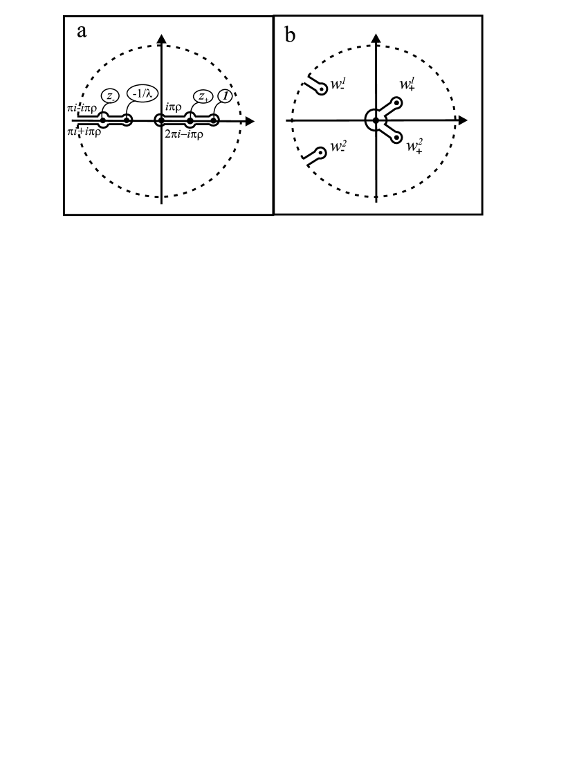
Figure 2: The domains $\mathbb{D}_{z}$ (a) and $\mathbb{D}_{w}$ (b).

Going around the branch cut $[0,1]$ the value of $\arg\left[w(z)\right]$ changes by $2\pi$ exactly once. Therefore, no repetition in the value of $w(z)$ can occur, i.e. the mapping $w(z)$ is schlicht (one-sheet). Hence the mapping $w(z)$ is bijective and one can construct an analytic, monovalued, schlicht mapping $w^{-1}(\cdot):\mathbb{D}_{w}\rightarrow\mathbb{D}_{z},$ inverse of$\ w(z)$. Then, given a complex number $a\in\mathbb{D}_{w}$, the equation $w(z)=a$ has a unique simple root $z(a)\in\mathbb{D}_{z}$, being an analytic function of $a$ in $\mathbb{D}_{w}$.

Thus, given a value of $C$, each root of (60) is the unique simple root of (62) for some $k$, and all the roots are different for different $k$-s. To solve the Bethe equations one formally can choose $P$ integers $k_{1},\ldots,k_{P}$ from the set $1,\ldots,L$. Then, substituting

$$z_{j}=w^{-1}\left[\exp\left(2\pi\mathrm{i}k_{j}/L\right)C^{1/L}\right]$$ (69)

into the constraint (58) for all $j=1,\ldots,P$, one obtains a unique equation for the parameter $C$. Solving the equation for $C$, we obtain the solutions corresponding to given set $k_{1},\ldots,k_{P}$. Going through all the possible sets of integers $k_{1},\ldots,k_{P}$ we obtain all the solutions of the Bethe equations.

It is easily seen that the eigenvectors (20,25) identically vanish on the solutions corresponding to the sets $k_{1},\ldots,k_{P}$ containing a pair of two equal integers, $k_{i}=k_{j}$, which result in $z_{i}=z_{j}$. Therefore one has to look over only those sets $k_{1},\ldots,k_{P}$, where all the numbers are different. If we assume that for any set the equation for $C$ has exactly one solution we obtain just as many solutions as we need (36) to obtain the complete set of linearly independent eigenvectors. The direct proof of this fact however is beyond the aims of present article and will be considered elsewhere.

Remark 2

For generic values of the parameter $\gamma$, and hence of the parameter $C$, the r.h.s. of (62) is away from the branch points of $w^{-1}(z)$, which ensures that the root of (62) is simple. However, for specific values of $\gamma$ this can be not the case. This does not create a problem as this situation can be considered as the limiting case of the generic one. In particular, a double root can appear at $z_{+}$ or $z_{-}$, as a consequence of square root singularities of $w^{-1}(z)$. In this case, one can think of it as a pair of roots at different banks of the branch cut. This in fact specifies the way in which it evolves when the value of $\gamma$ changes. Also the limit $C\rightarrow 0$, which implies $\gamma\rightarrow 0$, corresponds to $P$ roots meeting at $z=1$. Then, the choice of different integers $k_{i}$ for different roots $z_{i}$ removes the degeneracy as the arguments of $(z_{i}-1)$ are different.

Let us consider the curve $\Gamma_{c}$ defined by the equation

$$\left|w\left(z\right)\right|=c,$$ (70)

where $c$ is a real, positive number. All the roots are located on curves where $c=\left|C^{1/L}\right|$, for some discrete set of values of $C$ related to the solution via the equation (58). The particular case $\lambda=0$ of $\Gamma_{c}$ was named in [6] as the generalized Cassini oval. To describe the form of this curve, let us first look at the behaviour of $\left|w\left(z\right)\right|$ at the real axis. It is easily seen that $\left|w\left(z\right)\right|$ has two zeroes at the points $z=0$ and $z=1$, and diverges for $z\rightarrow\pm\infty$ and $z\rightarrow-1/\lambda$. There are also two extremums: $z_{+}$ and $\ z_{-}$ given by (64), which are a minimum and a maximum respectively. As $\rho$ varies from $0$ to $1$, the point $z_{+}$ monotonously moves from $1$ to $0$ and $z_{-}$ from $-1/\lambda$ to $-\infty$. At the same time $\left|w\left(z_{+}\right)\right|$ increases from zero for $0<\rho<1/2$, reaches the maximum at $\rho=1/2$ and then decreases back to zero for $1/2<\rho<1$, while $\left|w\left(z_{-}\right)\right|$ decreases from infinity for $0<\rho<1/2$, reaches the minimum at $\rho=1/2$ and then increases back to infinity for $1/2<\rho<1$. Note that the values of $\left|w\left(z_{+}\right)\right|$ and $\left|w\left(z_{-}\right)\right|$ meet only in one point $\rho=1/2$ approaching its values from below and above respectively. Let us look at the cross points of the plots $y=\left|w\left(x\right)\right|$ and $y=c$ as the constant $c$ grows starting from zero.

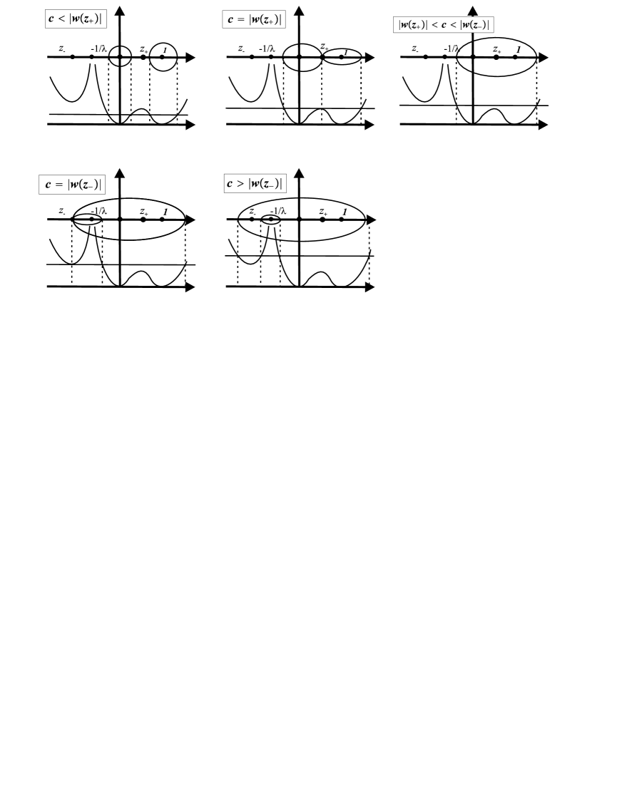
Figure 3: Schematic picture of the stages of the evolution of the contour $\Gamma_{c}$ as $c$ grows from zero to infinity. At the lower plots the the graphs $y=|w(x)|$ and $y=c$ are shown for each stage, which cross points define the cross points of $\Gamma_{c}$ with the real axis.

The following stages exist (see figure 3):

$c<\left|w(z_{+})\right|$

For small $c$ there are four cross points $\{-1/\lambda<z_{1}<0,$ $0<z_{2}<z_{3}<1,$ $1<z_{4}\}$, which corresponds to two ”ovals” encircling the origin and the point $z=1.$ In the limit $c\rightarrow 0$ the form of the contours approaches circles of vanishing radius collapsing to the points $z=0,1$. As the value of $c$ increases the point $z_{2}$ and $z_{3}$ move towards each other, and the radius of the ”ovals” increases .

$c=\left|w(z_{+})\right|$

When the value of $c$ reaches $\left|w(z_{+})\right|$, the points $z_{2}$ and $z_{3}$ merge at $z_{+}$, i.e. the two ”ovals” develop cusps meeting at $z_{+}$. Then the shape of the curve resembles the lemniscate. This form survives, when one considers the thermodynamic limit. Specifically, the right part of the curve is the one considered in studies of low lying eigenstates [3].

$\left|w(z_{+})\right|<c<\left|w(z_{-})\right|$

As $c$ exceeds $\left|w(z_{+})\right|$ the crosspoints $z_{2}$,$z_{3}$ disappear after merging at $z_{+}$such that only the two, $\left\{-1/\lambda<z_{1}<0,1<z_{4}\right\}$ remain. These are two crosspoints with the horizontal axis of the ”big oval”, which appears after the two ”smaller ovals” merge. The big oval contains the points $z=0,1$ inside, while the point $z=-1/\lambda$ stays outside. As $c$ increases $z_{1},z_{4}$ move along the real axis towards $-1/\lambda$ and $+\infty$ respectively. As the point $z_{1}$ is confined between $0$ and $-1/\lambda$, while the effective radius of the ”oval” is unbounded, it finally starts to bend around $-1/\lambda$ and approaches the real axis from below and above at the right of the point $-1/\lambda$.

$c=\left|w(z_{-})\right|$

At this stage the two points at the parts of the ”oval” bending around $-1/\lambda$ meet at $z_{-}$, so that two ”ovals” appear, one inside the other. They have sharp cusps at their only common point $z_{-}$ . The bigger ”oval” goes around $-1/\lambda,0,1$ while the smaller encircles only $-1/\lambda$.

$c>\left|w(z_{-})\right|$

After forming two ovals at previous stage, they detach from each other by splitting the common cross point with the real axis at $z_{-}$ into two new cross points $z_{2}^{\prime},z_{3}^{\prime}$, which then move along the real axis to $-\infty$ and $-1/\lambda$ respectively as $c$ go on growing. The form of the contours then approach two circles of infinite and zero radia, the latter collapsing to the point $-1/\lambda$.

In the case $\rho=1/2$, when the values of $\left|w\left(z_{+}\right)\right|$ and $\left|w\left(z_{-}\right)\right|$ are equal, the second and the fourth stages coincide while the third one does not take place.

An important point of the above analysis is the limiting shape of the curves under consideration as $c$ goes to zero or infinity. Specifically, one can always choose a value of $c$ so small that the contour $\Gamma_{c}$ separates a small neighborhood of the points $0$ and $1$ from the rest of the complex plane. For $c$ large, the same is valid for the points $-1/\lambda$ and $\infty$. This fact will be used in the next section to evaluate the sum over the Bethe roots.

5 Summation over the Bethe roots.

Let us rewrite the Bethe equations in terms of the variables $\left\{z_{i}\right\}$, given by(57), in polynomial form

$$P_{i}(Z)=0,$$ (71)

where it is convenient to write the polynomials $P_{i}(Z)$ as a difference of two other polynomials

$$P_{i}(Z)\equiv g_{i}\left(Z\right)-h_{i}\left(Z\right)$$ (72)

which read as follows

$$g_{i}\left(Z\right) = e^{-L\gamma}z_{i}^{L-P}\left(z_{i}-1\right)^{P}\prod\limits_{j=1}^{P}z_{j}\left(1+z_{j}\lambda\right),$$ (73)

$$h_{i}\left(Z\right) = \left(-1\right)^{P-1}\left(1+z_{i}\lambda\right)^{P}\prod\limits_{j=1}^{P}\left(z_{j}-1\right).$$ (74)

The aim of the present section is to evaluate the sum of the analytic functions over the roots of the system (71). Two remarks are necessary. First, we imply that the roots are bounded from infinity, as otherwise the eigenvectors and eigenvalues would be singular. Second, the polynomial equations can be satisfied with the solutions constructed from the roots from the set $\{0,-1/\lambda,1\}$. Furthermore, it is easy to see that if one of the roots $z_{i}$ is taken from this set, the other $P-1$ roots must belong to this set as well. However, solutions constructed in this way obviously do not match the constraint (52) for $\gamma\neq 0$, and, therefore, must be excluded. Appearance of extra solutions is due to multiplication of the BE by an expression that itself can be zero, when transforming it to the polynomial form. In the case $\gamma=0$ one such a solution exists. Namely it is $z_{1}=\cdots=z_{P}=1$, which corresponds to the ground state of the evolution operator, i.e. the stationary state of the stochastic process. As will be seen below, this case can be treated as a limiting case of the generic situation and does not require a special consideration.

Let us define the domain $D$ $\subset\mathbb{C}$ of the complex plane by the inequalities

$$D=\left\{z:a\leq\left|w(z)\right|\leq A\right\},$$ (75)

where $a$ and $A$ are two real positive constants, such that $a<A$. Denote by $\Gamma_{c}$ the contour discussed in the previous section, defined by (70)

$$\Gamma_{c}=\left\{z:\left|w(z)\right|=c\right\}.$$ (76)

Then the domain $D$ is between $\Gamma_{a}$ and $\Gamma_{A}$, and its boundary

$$\partial D=\left\{z:\Gamma_{a}\cup\Gamma_{A}\right\}$$ (77)

is oriented in such a way that going along it in positive direction one keeps the interior of $D$ left. Then we form a polycylinder domain $\mathbf{\Omega\subset}\mathbb{C}^{P}$ as a cartesian product of $P$ copies of $D$

$$\mathbf{\Omega}=D_{1}\times\cdots\times D_{P}.$$ (78)

The skeleton $\mathbf{\Gamma}$ of $\Omega$ is the subset of its boundary $\partial\mathbf{\Omega}$ consisting of points, which are at the boundary of every $D_{1},\ldots,D_{P}$:

$$\mathbf{\Gamma}=\partial D_{1}\times\cdots\times\partial D_{P}.$$

The definition (75) of $D$ guarantees that all the points $Z=\left(z_{1},\ldots,z_{P}\right)$, such that $z_{i}\in\{0,-1/\lambda,1,\infty\}$ for some $i$, are outside of  $\Omega$. On the other hand, the dimension of the complement of $\Omega$ approaches $P-1$ as $a$ and $A$ go to zero and infinity respectively, i.e. their Lebesgue measure in $\mathbb{C}^{P}$ vanishes. Thus, it is natural to expect that for $a$ small and $A$ large enough all the roots of the system (71) fall into $\mathbf{\Omega}$. Then, the sum of an analytic in $\mathbf{\Omega}$ function $f(Z)$ over the roots of BE which fall into $\mathbf{\Omega}$ can be evaluated with the aid of the multi-dimensional logarithmic residue theorem [9].

Theorem 3

Let $\Omega$$\subset$ $\mathbb{C}^{P}$ be a polycylinder domain with piecewise smooth boundary $\partial\mathbf{\Omega}$ and $\mathbf{\Gamma}$ be its skeleton. Let the mapping $\left\{P_{i}(Z),i=1,\ldots,P\right\}:\mathbf{\Omega}\rightarrow\mathbb{C}^{P}$ be holomorphic in $\mathbf{\Omega}$ and have no zeroes at the boundary $\partial\mathbf{\Omega}$. Then, for any function $f(Z)$ analytic in $\mathbf{\Omega}$, the sum of its values over the set $\mathcal{Z}=\left\{Z\in\mathbf{\Omega:}P_{i}\left(Z\right)=0,i=1,\ldots,P\right\}$ is given by the following integral

$$\sum_{Z\in\mathcal{Z}}f(Z) = \frac{1}{\left(2\pi\mathrm{i}\right)^{P}}\int_{\Gamma}f(Z)\frac{dP_{1}(Z)}{P_{1}(Z)}\wedge\cdots\wedge\frac{dP_{P}(Z)}{P_{P}(Z)}$$ (79)

$$= \int_{\Gamma}\frac{f(Z)}{\prod\nolimits_{i=1}^{P}P_{i}\left(Z\right)}\det\left[\frac{\partial P_{i}\left(Z\right)}{\partial z_{j}}\right]_{1\leq i,j\leq P}\prod\limits_{i=1}^{P}\frac{dz_{i}}{2\pi\mathrm{i}}.$$

Every zero is counted as many times as its multiplicity is.

The theorem is a particular case of the Caccippolly, Martinelly, Bishop, Sorani theorem, see [9]. The original theorem is proved for the domain called special analytic polyhedra, which in particular ensures the absence of zeroes of the mapping at the boundary of domain, which in turn guarantees that all zeroes inside the domain are the isolated ones. In our case the absence of zeroes at the boundary $\partial\mathbf{\Omega}$ of the domain $\mathbf{\Omega}$, is provided by the following lemma.

Lemma 4

Let $\mathbf{\Omega}$ be defined as above. Let $\lambda<1$. Then in the range of $\gamma:\left(\rho^{-1}\left|\ln\lambda\right|>\gamma>0\right)$, there exist constants $a_{0}$ and $A_{0},$ such that for any $a<a_{0}$ and $A>A_{0}$ the mapping $\left\{P_{1}(Z),\ldots,P_{P}(Z)\right\}$ has no zeroes on $\partial\mathbf{\Omega}$.

Proof. Suppose there is a point $Z=\left\{z_{1},\ldots,z_{P}\right\}\in\partial\mathbf{\Omega}$, such that $P_{i}(Z)=0$ for $i=1,\ldots,P$. It implies that

$$\left|\frac{g_{i}(Z)}{h_{i}\left(Z\right)}\right|\equiv e^{-L\gamma}\left|w(z_{i})\right|^{L}\left|\frac{z_{1}\cdots z_{P}}{w(z_{1})\cdots w(z_{P})}\right|^{1/\rho}=1.$$ (80)

The point $Z$ being at the boundary $\partial\mathbf{\Omega}$ of the domain $\mathbf{\Omega}$ means that at least one coordinate $z_{i}$ from the set $z_{1},\ldots,z_{P}$ is at the boundary of $D_{i}$, i.e. is either on $\Gamma_{a}$ or $\Gamma_{A}$. Let first

$$z_{i}\in\Gamma_{a}$$ (81)

for some $i$. As $z_{i}$ enters into (80) only via $\left|w(z_{i})\right|^{L}$, while the other factors do not depend on the index $i$ at all, $\left|w(z_{i})\right|^{L}$ does not depend on $i$ either, i.e. (81) holds for all $i=1,\ldots,P,$ which immediately yields

$$\left|z_{1}\cdots z_{P}\right|^{1/\rho}=e^{L\gamma}.$$ (82)

Recall that $a$ always can be chosen small enough such that $\Gamma_{a}$ belongs to small neighborhoods of the points $z=0$ and $z=1$. In other words for any small $\varepsilon>0$ one can choose a small $a_{0}$ such that for any $a<a_{0}$

$$\sup_{\left\{z\in\Gamma_{a}\right\}}\left|z\right|<1+\varepsilon.$$ (83)

Taking $\varepsilon<\left(e^{\gamma\rho}-1\right)$ we obtain

$$\left|z_{1}\cdots z_{P}\right|^{1/\rho}<e^{\gamma L},$$ (84)

which contradicts (82).

Consider now the case when $z_{i}\in\Gamma_{A}$ for some $i$. Analogously to the previous case one needs to satisfy (82) with the set of solutions $z_{1},\ldots,z_{P}$, which are on $\Gamma_{A}$, i.e. either go to infinity or to $\left(-1/\lambda\right)$, as $A$ increases. Thus, for any $\varepsilon>0$ one can always choose a large $A_{0}$ such that for any $A>A_{0}$

$$\inf_{\left\{z\in\Gamma_{A}\right\}}\left|z\right|>\left|\frac{1}{\lambda}\right|-\varepsilon.$$ (85)

Taking $\varepsilon<\left(\left|1/\lambda\right|-e^{\gamma\rho}\right)$ we obtain

$$\left|z_{1}\cdots z_{P}\right|^{1/\rho}>e^{\gamma L},$$ (86)

which also contradicts with 82.   

This lemma in particular ensures that the constants $a$ and $A$ always can be chosen small and large respectively, so that all the solutions of BE, are inside $\mathbf{\Omega}$. Indeed, according to the previous section the solutions always belong some contour $\Gamma_{c}$ for a particular value of $c$. Hence they would belong to the boundary of $\mathbf{\Omega}$ defined with $c=a$ or $c=A$. As follows from the above lemma no such solutions exist for $a<a_{0}$ and $A>A_{0}$. Therefore all the solutions are in $\mathbf{\Omega}$ defined with such $a$ and $A$.

The next lemma provides a condition for evaluating the integral in (79) in the form of infinite series.

Lemma 5

Let the domain $\mathbf{\Omega}$ and its skeleton $\Gamma$ be defined as above. Let the range of parameters be

$$0 \leq \lambda<1,$$ (87)

$$\rho^{-1}\left|\ln\lambda\right| < \gamma<0$$ (88)

and

$$\rho\leq\frac{1}{2}.$$ (89)

Then, one can choose the constants $a$ and $A\$such that for any $Z\in\Gamma$ the following conditions hold:

$$\left|\frac{g_{i}(Z)}{h_{i}\left(Z\right)}\right|<1$$ (90)

if $z_{i}\in\Gamma_{a}$ and

$$\left|\frac{g_{i}(Z)}{h_{i}\left(Z\right)}\right|>1$$ (91)

if $z_{i}\in\Gamma_{A}$ Furthermore the limits $a\rightarrow 0$ and $A\rightarrow\infty$ can be taken simultaneously, in such a way, that these inequalities hold.

Proof. It follows from the explicit form of $w(z)$ that for any $\varepsilon>0$ one can choose $a$ so small that

$$\inf_{z\in\Gamma_{a}}\left|z\right| > \left(1-\varepsilon\right)a^{\frac{1}{1-\rho}}$$ (92)

$$\sup_{z\in\Gamma_{a}}\left|z\right| < \left(1+\varepsilon\right).$$ (93)

On the other hand for any $\varepsilon>0$ one can choose $A$ so large that

$$\inf_{z\in\Gamma_{A}}\left|z\right| > \frac{(1-\varepsilon)}{\lambda}$$ (94)

$$\sup_{z\in\Gamma_{A}}\left|z\right| < \left(1+\varepsilon\right)\lambda^{\frac{\rho}{1-\rho}}A^{\frac{1}{1-\rho}}.$$ (95)

Let us write $c_{i}=a$ if $z_{i}\in\Gamma_{a}$ and $c_{i}=A$ if $z_{i}\in\Gamma_{A}$. Then we have

$$\left|\frac{g_{i}(Z)}{h_{i}\left(Z\right)}\right|=e^{-L\gamma}c_{i}^{L}\left|\frac{z_{1}\cdots z_{P}}{c_{1}\cdots c_{P}}\right|^{1/\rho},$$ (96)

Now we can use the inequalities (92) and (94) to estimate the bounds for the ratios $\left|z_{i}/c_{i}\right|$, which yield

$$~{}\left[\left(1-\varepsilon\right)\min\left(a^{\frac{\rho}{1-\rho}},\frac{1}{\lambda A}\right)\right]^{P}<\left|\frac{z_{1}\cdots z_{P}}{c_{1}\cdots c_{P}}\right|^{1/\rho}<\left[\left(1+\varepsilon\right)\max\left(\left(\lambda A\right)^{\frac{\rho}{1-\rho}},\frac{1}{a}\right)\right]^{P}.$$ (97)

If we choose $A$ and $a$ such that

$$\left(\lambda A\right)^{\frac{\rho}{1-\rho}}\leq\frac{1}{a},$$ (98)

then for $c_{i}=a$ we have

$$e^{-L\gamma}c_{i}^{L}\left|\frac{z_{1}\cdots z_{P}}{c_{1}\cdots c_{P}}\right|^{1/\rho}<\left(1+\varepsilon\right)^{L}e^{-L\gamma}<1,$$ (99)

which is (90). At the same time if we choose them such that

$$a^{\frac{\rho}{1-\rho}}\geq\frac{1}{\lambda A},$$ (100)

then for $c_{i}=A$ we have

$$e^{-L\gamma}c_{i}^{L}\left|\frac{z_{1}\cdots z_{P}}{c_{1}\cdots c_{P}}\right|^{1/\rho}>e^{-L\gamma}\left(\frac{1-\varepsilon}{\lambda}\right)^{L}>1,$$ (101)

which is (91). The only what we need is to satisfy both conditions (98) and (100) simultaneously, which implies

$$\left(\lambda A\right)^{-1}\leq a^{\frac{\rho}{1-\rho}}\leq\left(\lambda A\right)^{-\left(\frac{\rho}{1-\rho}\right)^{2}}.$$ (102)

This is possible if $\rho\leq 1/2$.   

Remark 6

The limit $\gamma\rightarrow 0$ in two above lemmas can be considered after the limits $a\rightarrow 0$ and $A\rightarrow\infty$ are taken. This particularly solves the problem of the groundstate mentioned above. While for $\gamma>0$ the roots corresponding to the groundstate are away from $Z=(1,\ldots,1)$, they approach this point when $\gamma$ approaches zero. However due to the order of limits described they still remain separated from this point by the boundary of $\mathbf{\Omega}$.

Using lemma 5, we can represent the factor $1/P_{i}(Z)$ under the integral in (79) in the form of infinite sum. Indeed, for $z_{i}\in\Gamma_{a}$ we have

$$\frac{1}{P_{i}(Z)}=\frac{1}{g_{i}\left(Z\right)-h_{i}\left(Z\right)}=-\frac{1}{h_{i}\left(Z\right)}\sum\limits_{n=0}^{\infty}\left(\frac{g_{i}\left(Z\right)}{h_{i}\left(Z\right)}\right)^{n},$$ (103)

while for $z_{i}\in\Gamma_{A}$

$$\frac{1}{P_{i}(Z)}=\frac{1}{g_{i}\left(Z\right)-h_{i}\left(Z\right)}=\frac{1}{h_{i}\left(Z\right)}\sum\limits_{n=-\infty}^{-1}\left(\frac{g_{i}\left(Z\right)}{h_{i}\left(Z\right)}\right)^{n}.$$ (104)

Thanks to (99,101), the series are absolutely and uniformly convergent, and, as such, can be integrated term by term. Note that the summands have no singularities in $\mathbf{\Omega}$. Therefore the contours $\Gamma_{a}$ and $\Gamma_{A}$ can be deformed into a single contour. With respect to singularities of the expression under the integral, it has the same form as the contour $\Gamma^{\infty}$ described in the Section 3, which was used to construct the resolution of the identity operator in the case of infinite lattice. Thus, both the contours $\Gamma_{a}$ and $\Gamma_{A}$ can be deformed into $\Gamma^{\infty}$ and the term corresponding to the integral over $\Gamma_{a}$ brings a minus sign due to the opposite orientation. The final expression has no dependence on the values of $a$ and $A$. Therefore, assuming the limit $a\rightarrow 0,A\rightarrow\infty$ one can think of $\Omega$ as of product of $P$ complex plains punctured in four points $\left\{0,1,-1/\lambda,\infty\right\}$, which clearly contains all the necessary solutions of the BE. As a result we have the following expression for the sum over the roots of the Bethe equations.

Theorem 7

The sum of the values of a function $f(Z)$ analytic in the whole complex plane, except maybe the points $\left\{0,1,-1/\lambda,\infty\right\}$, over the roots of the Bethe equations is given by the following $P$-tuple absolutely converging sum.

$$\sum_{Z\in\mathcal{Z}}f(Z) = \sum\limits_{n_{1}=-\infty}^{\infty}\cdots\sum\limits_{n_{P}=-\infty}^{\infty}\int_{\Gamma_{1}^{\infty}\times\cdots\times\Gamma_{P}^{\infty}}f(Z)\prod\nolimits_{i=1}^{P}\left(\frac{h_{i}(Z)}{g_{i}(Z)}\right)^{n_{i}}$$ (105)

$$\times\det\left[\frac{\partial\left(\ln g_{k}(Z)-\ln h_{k}(Z)\right)}{\partial z_{j}}\right]_{1\leq k,j\leq P}\prod\limits_{l=1}^{P}\frac{dz_{l}}{2\pi\mathrm{i}},$$

Note that we write $\partial\left(\ln g_{k}(Z)\right)/\partial z_{j}\equiv\left(\partial g_{k}(Z)/\partial z_{j}\right)/g_{k}(Z)$ in the determinant instead of $\left(\partial g_{k}(Z)/\partial z_{j}\right)/h_{k}(Z)$, because the equality $h_{k}(Z)=g_{k}(Z)$ holds on the roots of BE, which are the only contributing the integral.

6 Proof of the resolution of the identity and formula for the transition probability

Now, we are in a position to write the sum in (55) in the integral form (105) substituting

$$f(Z)=\frac{\left\langle X|B_{Ze^{-\gamma}}^{\gamma}\right\rangle\left\langle\overline{B}_{Ze^{-\gamma}}^{\gamma}|Y\right\rangle}{\left\langle\overline{B}_{Ze^{-\gamma}}^{\gamma}|B_{Ze^{-\gamma}}^{\gamma}\right\rangle}.$$ (106)

To this end we need the expression for the norm $\left\langle\overline{B}_{Ze^{-\gamma}}^{\gamma}|B_{Ze^{-\gamma}}^{\gamma}\right\rangle$. The hypothesis about the form of the norms of Bethe vectors was first proposed by Gaudin [10, 11]. Later it was proved by Korepin [12] within the quantum inverse scattering method for XXX and XXZ type models. Those results can be applied to our model with minor changes. However, they require developing the quantum inverse scattering method, which is not a subject of the present article, and will be done elsewhere. Here we use the formulas as they are given in the Korepin’s article. Note that the proof below and of the final result do not rely on the validity of the formula for the norm. The latter serves as a hint for writing the expression under the integral, while the validity of the results follows from the resolution of the identity proof made independently. Written in the the transformed variables (57), Gaudin formula yields

$$\left\langle\overline{B}_{Ze^{-\gamma}}^{\gamma}|B_{Ze^{-\gamma}}^{\gamma}\right\rangle=\det\left[z_{i}\frac{\partial}{\partial z_{i}}\ln\frac{g_{j}(Z)}{h_{j}(Z)}\right]_{i,j=1,\ldots,P},$$ (107)

which being in the denominator of the expression under the integral cancels the Jacobian in the numerator, yielding only the factor $\left(z_{1}\cdots z_{P}\right)^{-1}$. Substituting the explicit form of the eigenvectors (20,25) and the functions $g(z)$ and $h(z)$, (73,74), and performing one summation over the permutations, which is trivial due to the permutation symmetry of the summands, we come to the following expression.

$$~{}\sum\limits_{Z\in\mathcal{Z}}\frac{\left\langle X|B_{Z}^{\gamma}\right\rangle\left\langle\overline{B}_{Z}^{\gamma}|Y\right\rangle}{\left\langle\overline{B}_{Z}^{\gamma}|B_{Z}^{\gamma}\right\rangle}=W(X)\sum\limits_{n_{1}=-\infty}^{\infty}\cdots\sum\limits_{n_{P}=-\infty}^{\infty}\left(-1\right)^{(P-1)\sum_{k=1}^{P}n_{k}}\sum\limits_{\sigma\in S_{P}}\left(-1\right)^{|\sigma|}$$ (108)

$$\times\prod\nolimits_{i=1}^{P}\int_{\Gamma^{\infty}}\left(\frac{1+\lambda z_{i}}{1-1/z_{i}}\right)^{i-\sigma_{i}+Pn_{i}-\sum_{l=1}^{P}n_{l}}\left(e^{-\gamma}z_{i}\right)^{-x_{i}+y_{\sigma_{i}}-Ln_{i}}\frac{dz_{i}}{2\pi iz_{i}}.$$

Though there is an infinite $P$-tuple sum, it turns out that only few terms in each sum contribute. The following lemma establishes which summands are nonzero.

Lemma 8

Let $X,Y\in\mathbb{Z}_{<,L}^{P}$ be two particle configurations, $\sigma$ be a permutation $\left(\sigma_{1},\ldots,\sigma_{P}\right)$ of the integers $1,\ldots,P$, $\left\{n_{1},\ldots,n_{P}\right\}\in\mathbb{Z}^{P}$ be a set of integers. Then, the necessary conditions for the product

$$\prod\nolimits_{i=1}^{P}\int_{\Gamma^{\infty}}\left(\frac{1+\lambda z_{i}}{1-1/z_{i}}\right)^{i-\sigma_{i}+Pn_{i}-\sum_{k=1}^{P}n_{k}}\left(e^{-\gamma}z_{i}\right)^{-x_{i}+y_{\sigma_{i}}-Ln_{i}}\frac{dz_{i}}{2\pi\mathrm{i}z_{i}}$$ (109)

to be nonzero are

$$n_{i}\in\left\{-1,0,1\right\}$$ (110)

for $i=1,\ldots,P$.  Furthermore, the cases when $n_{i}=\pm 1$ for some $i=1,\ldots,P,$ suggest that

$$\sum_{i=1}^{P}n_{i}=0$$

and there are clusters in the configurations $X$ and $Y$, which in particular contain the sites $1$ and $L$.

Proof. To evaluate the integrals over $\Gamma^{\infty}$ under the product we expand the expression under the integral into the Laurent series in the ring $1<\left|z\right|<1/\lambda$, implying $\lambda>1$, and look for the coefficient coming with $z^{-1}$. Let us for brevity introduce the notations

$$a_{ij} = i-j+Pn_{i}-\sum_{k=1}^{P}n_{k},$$ (111)

$$b_{ij} = x_{i}-y_{j}+Ln_{i}.$$ (112)

Then, the integrals to be nonzero, the following conditions must be met:

$$\textrm{a. \ \ \ if \ }a_{i\sigma_{i}} = 0,\textrm{ \ then \ }b_{i\sigma_{i}}=0;$$ (113)

$$\textrm{b. \ \ \ if \ }a_{i\sigma_{i}} > 0,\textrm{ \ then \ }b_{i\sigma_{i}}\leq a_{i\sigma_{i}};$$ (114)

$$\textrm{c. \ \ \ if \ }a_{i\sigma_{i}} < 0,\textrm{ \ then \ }b_{i\sigma_{i}}\geq a_{i\sigma_{i}}.$$ (115)

Given particle configurations $X,Y$ and a permutation $\sigma$, every element from the set $\{n_{i}\}_{i=1,\ldots,P}$ fall into one of three classes (a),(b) or (c) depending on the sign of $a_{i\sigma_{i}}$. Then the inequalities (113-115) determine which restrictions on $n_{i}$ must be imposed, all the integrals in the product to be nonzero simultaneously.

First we note that as the coordinates of particles on the finite lattice satisfy $\left|x_{i}-y_{j}\right|<L$, the only way to satisfy the equality $b_{i\sigma_{i}}=0$ is to put $n_{i}=0$. Therefore, this is always the case for the numbers $n_{i}$, which belong to the class (a).

One can use a similar argument to consider a particular case of the set $\{n_{i}\}_{i=1,\ldots,P}$ with all components equal.

$$n_{1}=n_{2}=\ldots=n_{P}\equiv n.$$ (116)

Then for such $i$ that $a_{i\sigma_{i}}=\left(i-\sigma_{i}\right)>0$, class (b), (114) requires $n\leq 0$, while for such $j$ that $a_{j\sigma_{j}}=\left(j-\sigma_{j}\right)<0$, class (c), (115) implies $n\geq 0$. Apparently for any permutation $\sigma$, where for some $i$ there is a number $\sigma_{i}$ which satisfies $\left(i-\sigma_{i}\right)\geq 0$, there must be at least one $j$ such that $\left(j-\sigma_{j}\right)\leq 0$. Thus we necessarily have $n=0$.

To study the other sets we estimate the bounds of their maximal and minimal elements. Consider the sets $\{n_{i}\}_{i=1,\ldots,P}$, where not all components are equal. From such set a maximal element can be chosen

$$n_{\max}\equiv\max\{n_{1},\ldots,n_{P}\}.$$ (117)

Of course, in general several numbers from the set can attend the maximum. The proof below consists of two steps. We first show that at least one of them falls either into the class (a) or into the class (b), i.e. satisfies either the first equality in (113) or the first inequality in (114). Then we find which restrictions on $n_{\max}$follow from the second equality of (113) or the second inequality (114).

To proceed with the first step we note that for any $k$ such that $n_{k}=$ $n_{\max}$ at least a part of $a_{k\sigma_{k}}$ is always positive

$$Pn_{k}-\sum_{l=1}^{P}n_{l}>0.$$ (118)

The remaining term $\left(k-\sigma_{k}\right)$, which also enters into $a_{k\sigma_{k}}$, is either positive or negative. In the case when it is positive or it is negative, but its absolute value is smaller then one of the other terms, we have $a_{k\sigma_{k}}\geq 0$. It can happen, however, that $\left(k-\sigma_{k}\right)$ is negative and its absolute value is large enough to turn $a_{k\sigma_{k}}$ to be negative. This is possible when

$$Pn_{k}-\sum_{k=1}^{P}n_{k}\leq\left|k-\sigma_{k}\right|\leq P-1.$$ (119)

Let $s$ be an integer, $1\leq s\leq P$, such that

$$Pn_{\max}-\sum_{k=1}^{P}n_{k}=P-s.$$ (120)

The last equation suggests that the number elements in the set $\{n_{i}\}_{i=1,\ldots,P}$ equal to $n_{\max}$ is at least $s$, i.e. there exists at least $s$ integers $1<k_{1},<\cdots<k_{s},\leq P$ such that

$$n_{k_{1}}=\cdots=n_{k_{s}}=n_{\max}.$$ (121)

Let us now check the sign of $a_{i\sigma_{i}}$ for $i$ chosen from $k_{1},\ldots,k_{s}$ and an arbitrary permutation $\sigma$. At worst we have $\sigma_{k_{1}}=P-s+1,\ldots,\sigma_{k_{s}}=P$, in which case for $i=k_{1}$, $a_{i\sigma_{i}}=\left[k_{1}-\left(P-s+1\right)\right]+\left(P-s\right)\geq 0$.  For any other $\sigma$ either $\sigma_{i}$ can be taken smaller or $i$ bigger, so the inequality becomes strict. Thus, we conclude that there is always at least one maximal element belonging either to the class (a) or (b), which finishes the first step of the proof.

According to the above arguments for the class (a) we get $n_{\max}=0$. Let now $n_{i}=n_{\max}$ be in the class (b). Combination of the second inequality (114) and the finite lattice restriction on the difference of the particle coordinates

$$\left|\left(x_{i}-y_{j}\right)-\left(i-j\right)\right|\leq L-P$$ (122)

give the upper bound for $n_{\max}$.

$$n_{\max}\leq 1-\frac{1}{L-P}\sum_{k=1}^{P}n_{k}.$$ (123)

All the above arguments can be applied also to the minimal element as well

$$n_{\min}\equiv\min\{n_{1},\ldots,n_{P}\},$$

so we conclude that it belongs either to the class (a), where $n_{\min}=0$ or to the class (c), where (115) and (122) yield

$$n_{\min}\geq-1-\frac{1}{L-P}\sum_{k=1}^{P}n_{k}.$$ (124)

It follows from (123) that if $\sum_{k=1}^{P}n_{k}$ is positive, then $n_{\max}$ must be strictly less than $1$ and hence nonsensitive. At the same time, one sees from (123) that if $\sum_{k=1}^{P}n_{k}$ is negative then $n_{\min}$ must be strictly greater than $-1$ and hence nonnegative. Thus the only possibility is to have

$$\sum_{k=1}^{P}n_{k}=0.$$ (125)

Substituting this back into (123,124) we conclude that there are only three possible values of the elements of the set $\{n_{i}\}_{i=1,\ldots,P}$

$$n_{i}\in\{-1,0,1\},\,\,i=1,\ldots,P,$$ (126)

the numbers $+1$ and $-1$ appearing in the set $\{n_{i}\}_{i=1,\ldots,P}$ equally many times.

Consider now the case when not all $n_{i}$ are equal to zero, i.e.

$$n_{\min}=-1,n_{\max}=1$$ (127)

If we return to the inequalities (114,115) and repeat the derivation of (123,124) using (125), we obtain that the case (127) is realized when the weak inequality (122) turns to the equality. Specifically, deriving the estimate for $n_{i}=n_{\max}=1$, the necessary condition for $n_{\max}$ to be equal to $1$ is

$$y_{\sigma_{i}}-x_{i}-(\sigma_{i}-i)=L-P.$$ (128)

This means that the particles with coordinates $x_{i}$ and $y_{\sigma_{i}}$ belong to the clusters in $X$ and $Y$, which spread to the last and the first sites respectively, i.e. the particle at $x_{i}$ belongs to the cluster of $X$, which starts with $x_{1}=1$ and the particle at $y_{\sigma_{i}}$ belongs to the cluster of $Y$, which ends with $y_{L}=L$. Similarly, for $n_{j}=n_{\min}=-1$ we have

$$y_{\sigma_{j}}-x_{j}-(\sigma_{j}-j)=-\left(L-P\right),$$

i.e. the particle at $x_{j}$ belongs to the cluster of $X$, which ends with $x_{L}=L$ and the particle at $y_{\sigma_{j}}$belongs to the cluster of $Y$, which starts with $y_{1}=1$. Thus we conclude that in both $X$ and $Y$ there exist the clusters, which cover at least the sites at the positions $1$ and $L$. This proves the last statement of the lemma.   

Of course the choice of the reference point at the ring has a conventional character. One can get reed of the terms $n_{i}=\pm 1$ by simple rotation, which places any hole of one of the configurations $X$ or $Y$ either into the site $1$ or $L$. This fact is useful for the proof of the resolution of the identity relation.

Theorem 9

The resolution of the identity operator is given by l.h.s of (54).

Proof. Consider the integral representation (108) of the sum in (54). According to the pervious lemma if one of the configurations $X$ and $Y$ are such that any of the sites $1$ and $L$ is empty the only term of the sum that remains corresponds to $n_{1}=\cdots=n_{P}=0$. This term coincides with the resolution of the identity operator for the infinite lattice. For the proof of the infinite lattice case we refer the reader to the Proposition 1 from our first paper [1].

The cases where in both configurations $X$ and $Y$ there is a cluster containing the sites $1$ and $L$ can be reduced to the previous situation by translation. Specifically we note that the product $\left\langle X|B_{Z}^{\gamma}\right\rangle\left\langle\overline{B}_{Z}^{\gamma}|Y\right\rangle$ is invariant under the translations, i.e.

$$\left\langle x_{1}+1,\ldots,x_{P}+1|B_{Z}^{\gamma}\right\rangle\left\langle\overline{B}_{Z}^{\gamma}|y_{1}+1,\ldots,y_{P}+1\right\rangle$$

$$= \left\langle X\mathbf{\tau}^{-1}|B_{Z}^{\gamma}\right\rangle\left\langle\overline{B}_{Z}^{\gamma}|\mathbf{\tau}Y\right\rangle=\tau_{Z}\tau_{Z}^{-1}\left\langle X|B_{Z}^{\gamma}\right\rangle\left\langle\overline{B}_{Z}^{\gamma}|Y\right\rangle$$

$$= \left\langle x_{1},\ldots,x_{P}|B_{Z}^{\gamma}\right\rangle\left\langle\overline{B}_{Z}^{\gamma}|y_{1},\ldots,y_{P}\right\rangle.$$

Hence we can repeatedly apply the translation operators $\mathbf{\tau}$ and $\mathbf{\tau}^{-1}$ until a hole comes either to the site $1$ or $L$. In this way the problem is reduced to the proved one.   

Since we have proven the formula for the resolution of the identity operators, we can apply it to find the matrix element we are looking for. To this end, as shown in (56) we must insert the eigenvalue of $\mathbf{T}_{\gamma}^{t}$ under the integral. Then the integral representation of $F_{t}^{\gamma}(X,t|Y,0)$ is

$$\left\langle X|\mathbf{T}_{\gamma}^{t}Y\right\rangle = \left(1+\lambda\right)^{-Pt}W(X)\sum\limits_{\sigma\in S_{P}}\left(-1\right)^{|\sigma|}$$ (129)

$$\times\int_{\Gamma}\prod\nolimits_{i=1}^{P}\frac{\left(e^{-\gamma}z_{i}\right)^{-x_{i}+y_{\sigma_{i}}}\left(1+\lambda z_{i}\right)^{i-\sigma_{i}+t}}{\left(1-1/z_{i}\right)^{i-\sigma_{i}}}\frac{h_{i}\left(Z\right)}{P_{i}\left(Z\right)}\frac{dz_{i}}{2\pi\mathrm{i}z_{i}}.$$

Going to the form of the $P$-tuple sum we have

$$\left\langle X|\mathbf{T}_{\gamma}^{t}Y\right\rangle=W(X)\sum\limits_{n_{1}=-\infty}^{\infty}\cdots\sum\limits_{n_{P}=-\infty}^{\infty}e^{\gamma\sum_{j=1}^{P}\left(x_{j}-y_{j}+Ln_{j}\right)}\left(-1\right)^{(P-1)\sum_{l=1}^{P}n_{l}}$$

$$\times\sum\limits_{\sigma\in S_{P}}\left(-1\right)^{|\sigma|}\prod\nolimits_{i=1}^{P}f(i-\sigma_{i}+Pn_{i}-\sum_{k=1}^{P}n_{k},x_{i}-y_{\sigma_{i}}+Ln_{i},t),$$ (130)

where

$$f(a,b,t)=\left(1+\lambda\right)^{-t}\int_{\Gamma^{\infty}}\left(1+\lambda z\right)^{t}\left(\frac{1+\lambda z}{1-1/z}\right)^{a}z^{-b}\frac{dz}{2\pi\mathrm{i}z}.$$ (131)

The integral for $f(a,b,t)$ is evaluated in terms of the hypergeometric functions (8). The sum over the permutations leads us to the determinant, given in (10). By putting $\gamma=0$ we obtain the result for conditional probability announced.

Like the sum obtained for the resolution of the identity operator, which is the particular case of the sum (130) at $t=0$, the latter sum being formally infinite, however contains finitely many nonzero terms. The analysis similar to one of the lemma 8 shows that at time $t$ the upper bound for the maximal element $n_{\max}(t)$ of the set $\{n_{i}\}_{i=1,\ldots,P}$, which ensures corresponding summand to be nonzero, is

$$n_{\max}(t)\leq 1-\frac{1}{\left(L-P\right)}\sum_{k=1}^{P}n_{k}+\frac{t}{\left(L-P\right)},$$ (132)

while that for minimal one, $n_{\min}(t)$, is still like it was for the $t=0$ case

$$n_{\min}\left(t\right)\geq-1-\frac{1}{\left(L-P\right)}\sum_{k=1}^{P}n_{k}.$$ (133)

The bounds for the sum $\sum_{k=1}^{P}n_{k}$ can be obtained from the following arguments. Suppose that $\sum_{k=1}^{P}n_{k}>t$. Then (132) requires $n_{\max}(t)\leq 0$, which contradicts the assumption. Thus we have

$$\sum_{k=1}^{P}n_{k}\leq t.$$ (134)

Another argument can be given, based on the fact that $\sum_{k=1}^{P}n_{k}\leq Pn_{\max}(t)$. Then using (132) we obtain

$$\sum_{k=1}^{P}n_{k}\leq P+\frac{t-P}{L}.$$ (135)

The first upper bound is lower than the second, when $t<P,$ and vice versa when $t>P$. For the lower bound we suppose that $\sum_{k=1}^{P}n_{k}<0$, which contradicts (133) and results in

$$\sum_{k=1}^{P}n_{k}\geq 0.$$ (136)

Finally we can use these inequalities to estimate the range of the summation indices corresponding to the summands, which give nonzero contribution.

Lemma 10

For the summands of the sum (130) to be nonzero it is necessary that

$$n_{i}\leq 1+\frac{t}{\left(L-P\right)},\,\,\sum_{k=1}^{P}n_{k}\geq 0$$ (137)

and

$$n_{i}\geq-1-\frac{t}{\left(L-P\right)},\,\,\sum_{k=1}^{P}n_{k}\leq t$$ (138)

if $P\leq t$ and

$$n_{i}\geq-1-\frac{P\left(L-P+t\right)}{L\left(L-P\right)},\,\,\sum_{k=1}^{P}n_{k}\leq P+\frac{t-P}{L}.$$ (139)

if $P>t$, for $i=1,\ldots,P$. In the cases, when the expressions in r.h.s. are not integer, the inequalities are strict.

From the definition of the generating function $F_{t}^{\gamma}(X,t|Y,0)$ one concludes that the coefficient of $e^{\gamma J}$ for some nonnegative integer $J$ is the probability $P_{t}(X,J;t|Y,0;0)$ for the total distance travelled by particles for time $t$ and the final configurations $X$, given the initial configuration is $Y$. One can see that in (130) the similar term is $e^{\sum_{i=1}^{P}\left(x_{i}-y_{i}+Ln_{i}\right)}$, while the probability for the travelled distance to be $J$ is the sum of the coefficients of terms, where the sum $n_{1}+\cdots+n_{P}$ is fixed, $\sum_{i=1}^{P}\left(x_{i}-y_{i}+Ln_{i}\right)=J$.  Thus, the sum $(n_{1}+\cdots+n_{P})$ has a meaning of the total number of windings around the lattice all the particles made. By this reason, the sum is always nonnegative unlike the individual numbers $n_{1},\ldots,n_{P}$. The meaning of the latter is well understood in frame of the geometric approach to the BA [1]. These are the winding numbers of ”virtual” free trajectories, which being weighted with corresponding weights can be used to reconstruct the TASEP dynamics.

7
Conclusion and discussion

To conclude we have obtained the probability of the transition from one configuration to another for arbitrary time for the TASEP with parallel update on a ring. To this end we developed the method of summation over the solutions of the Bethe equations, which is based on the multidimensional version of Cauchy residue theorem. In this way the integral representation of the solution is obtained. The expressions under the integral can be expanded into the uniformly convergent power series, which being integrated term by term, yields the result in form of multiple and formally infinite sum of the terms, each having the determinant form. It is shown that only finitely many terms of this sum are nonzero. Note that though the convergence of the series under the integral is proved for the domain $0\leq\rho\leq 1/2$, the behaviour of the final finite sums have no singularities at the point $\rho=1/2$ as well as for any values of $\rho$. Therefore we expect that arguments of analytic continuation exist which extend the proof for any value of density, $0\leq\rho\leq 1$. On the other hand the case $1/2\leq\rho\leq 1$ is related to $0\leq\rho\leq 1/2$ by particle hole symmetry. It is an interesting exercise to find an explicit relation between the final formulae of the transition probabilities for these two cases.

There are several directions of possible development of the result. First, it looks possible to generalize the method to extract not only the sum over the solutions of the BE, but also to extract the contribution of particular solutions. In this way one could obtain closed exact expressions for particular eigenvalues and eigenvectors, rather than only the asymptotic behaviour studied before. Second, the integral representation obtained can be useful to study the large time asymptotics for the growth phenomena with time. Many similar results where obtained recently for the infinite lattice, due to the observed parallels with the theory of random matrix ensembles [13, 14, 15, 16, 17, 18, 19]. The Bethe ansatz, giving the integral representations of the physical quantities like particle current probability distribution, could also be a starting point of such an asymptotical analysis. Particularly, the result of present paper could be used to make an advance for the ring geometry where not much results have been obtained yet.

References

- [1] Povolotsky A M and Priezzhev V B, 2006 J. Stat. Mech. P07002
- [2] Schütz G M, 1997 J. Stat. Phys. 88 427
- [3] Povolotsky A M and Mendes J F F, 2006 J. Stat. Phys. 123 125
- [4] Gwa L H and Spohn H, 1992 Phys. Rev. A 46 844
- [5] Derrida B and Lebowitz J L, 1998 Phys. Rev. Lett. 80 209
- [6] Golinelli O and Mallick K (2005) J. Phys. A: Math. Gen. 38 1419
- [7] Priezzhev V B Exact Non-Stationary Probabilities in the Asymmetric Exclusion Process on a Ring 2002 Preprint cond-mat/0211052
- [8] Priezzhev V B, 2003 Phys. Rev. Lett. 91 050601
- [9] Aizenberg I A and Yuzhakov A P, 1983 Integral representations and residues in multidimensional complex analysis (Translated from the Russian by H. H. McFaden. Translation edited by Lev J. Leifman. Translations of Mathematical Monographs, 58. American Mathematical Society, Providence, RI)
- [10] Gaudin M, 1983 La Fonction d’Onde de Bethe (Masson S. A., Paris)
- [11] Gaudin M, McCoy B M and Wu T T 1981 Phys. Rev. D 23 417
- [12] Korepin V E 1982 Cmmun. Math. Phys. 86 391
- [13] Johansson K, 2000 Comm. Math. Phys. 209 437
- [14] Rákos A and Schütz G M 2005 J. Stat. Phys. 118 511
- [15] Nagao T and Sasamoto T, 2004 Nucl. Phys. B 699 487
- [16] Praehofer M, Spohn H 2002 In and Out of Equilibrium, edited by V. Sidoravicius, Progress in Probability 51 185
- [17] Sasamoto T, 2005 J. Phys. A: Math. Gen. 38 L549
- [18] Ferrari P L and Spohn H 2006 Comm. Math. Phys. 265 1
- [19] Ferrari P L and Spohn H, 2005 J. Phys. A: Math. Gen. 38 L557