Positions of Point-Nodes in Borocarbide Superconductor YNi₂B₂C

Abstract

To determine the superconducting gap function of YNi₂B₂C, we calculate the local density of states (LDOS) around a single vortex core with the use of Eilenberger theory and the band structure calculated by local density approximation assuming various gap structures with point-nodes at different positions. We also calculate the angular-dependent heat capacity in the vortex state on the basis of the Doppler-Shift method. Comparing our results with the STM/STS experiment, the angular-dependent heat capacity and thermal conductivity, we propose the gap-structure of YNi₂B₂C, which has the point-nodes and gap minima along $\langle 110\rangle$. Our gap-structure is consistent with all results of angular-resolved experiments.

I Introduction

The discovery of the nonmagnetic borocarbide superconductor YNi₂B₂CCava has considerable attention because of the growing evidence for highly anisotropic superconducting gap and high superconducting transition temperature $15.5$ K. The boron isotope effect supports the classification of this material as electron-phonon mediated superconductor.Lawrie ; Cheon At an early stage, from specific heat, thermal conductivity, Raman scattering and photoemission spectroscopy experiments on YNi₂B₂C, a highly anisotropic gap function was concluded.Muller In recent years, Maki et al.MakiThal theoretically suggested that the gap symmetry of this material is $s$+$g$ wave and the gap function has zero points (point-nodes) in momentum space. Motivated by this prediction, field-angle-dependent heat capacity (FAD heat capacity)Park and angular variation of the thermal transport (AV thermal transport)Izawa on YNi₂B₂C have been measured and these results were considered to be consistent with this prediction. The FAD heat capacity and the AV thermal conductivity in $H$ rotated within the $ab$ plane show a fourfold oscillation with narrow cusps because of the presence of nodal quasiparticles subject to Doppler shifts. These results suggest that the gap function has point-nodes along the $a$ and $b$ axes. However, in the analysis of both experiments, the isotropic Fermi surface (FS) was assumed. YNi₂B₂C has highly anisotropic Fermi surfaces (FSs).Lee ; Singh ; Yamauchi

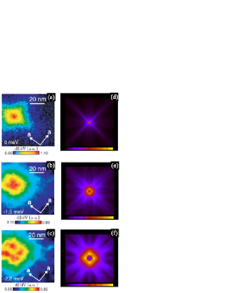
Figure 1: (Color Online) Tunneling conductance images observed by Nishimori et al. at 0.46K in 0.07 T ($72\times 72$nm) for the bias voltage (a) 0meV, (b)-1.5meV, (c)-2.2meV. In this figure, we quoted from Fig.5 (a), (c) and (e) in ‘First Observation of the Fourfold-symmetric and Quantum Regime Vortex Core in YNi₂B₂C by Scanning Tunneling Microscopy and Spectroscopy’ (H. Nishimori et al, Journal of the Physical Society of Japan 73, 3247 (2004)). The LDOS images calculated for (d)$\epsilon/\Delta_{\infty}=0$, (e)0.15, (f)0.3, where $4\sqrt{2}\xi_{0}\times 4\sqrt{2}\xi_{0}$ is shown. Here, $\Delta_{\infty}$ denotes a pair-potential in the bulk region averaged on the Fermi surface and $\xi_{0}$ denotes a coherent length. The smearing factor is $\delta=0.05\Delta_{\infty}$

The local density of states (LDOS) in the isolated vortex of YNi₂B₂C was measured at 0.46K by the scanning tunneling microscopy and spectroscopy (STM/STS).Nishimori The vortex core was found to be fourfold star-shaped in real space (see Fig. 1(a)-(c)). Near $E=0$meV, the LDOS extends toward $\langle 100\rangle$ (the $a$-axis) and has a peak at the center of the vortex core (Fig. 1(a)). With increasing energy, the peak of the LDOS splits into four peaks toward $\langle 110\rangle$ (Fig. 1(b),(c)). The anisotropic spatial pattern of the LDOS around a vortex core is a consequence of the anisotropic pair-potential and FS. Many theoretical studies have been done since the LDOS of NbSe₂ can be observed by STM/STS.Gygi ; Hayashi ; Schopohl ; Ichioka ; Caroli ; Kramer ; Nagai_ce ; Nagai ; Hess We have calculated the LDOS pattern around a vortex core of YNi₂B₂C, assuming that the gap symmetry is $s$+$g$-wave and the FS is isotropic.Nagai Since this result explains the STM results only partly, obviously the calculations of the LDOS with a highly anisotropic FS are needed.

The band structure for YNi₂B₂C has been calculated, on the basis of the local density approximation (LDA). Lee et al.Lee and Singh Singh obtained three bands (17th, 18th and 19th) with mainly Ni-3d and Y-4d character which cut across the Fermi level by using the linearized muffin-tin orbital method and the general potential linearized augmented plane wave method, respectively. In recent years, band structure calculations were carried out by Yamauchi et al.,Yamauchi who are some of the authors, by using a full potential LAPW(FLAPW) method. They have carried out LDA-based calculations with a certain modification to describe well the experimental FSs which are obtained by de Haas van Alphen effect. In this modification, Y-d and Ni-d levels are shifted upward from the original LDA levels by 0.11Ry and 0.05 Ry, respectively. Such the modification have been successful in the FS calculations in LaB₆,Harima1 YbAl₃Ebihara and LaRh₃B₂.Harima2 This shift may originate mainly in the self-interaction and/or the non-local corrections to the LDA. They have shown that the density of states from 17th band, which is related to a multiple connected electron FS, has a sharp peak at Fermi energy. This peak comes from a van Hove singularity around (1/5, 1/5, 0) point in k-space as we will explain later in this paper. They have suggested that this singularity may lead large electron- phonon coupling locally, and give rise to anisotropic gap behavior in the superconducting state.

The purpose of this paper is to determine the gap structure consistent with the STM/STS, the FAD heat capacity and the AV thermal transport experiments. We show the results of four calculations considering the band structure calculations. First, we calculate the LDOS pattern around a single vortex on the basis of the quasiclassical Eilenberger theory.Nagai We assume various gap structures, and finally obtain the gap structure which can explain the STM experiment. Second, we calculate the density of states in weak magnetic fields in the $a$-$b$ plane on the basis of the Doppler-shift method.Volovik We show that the FAD heat capacity and the AV thermal transport experiments are consistent with the angular dependence of the density of states from the gap structure consistent with the STM experiment in the presence of magnetic fields. Third, we show that the density of states from this gap structure is consistent with the STM experiment in the absence of magnetic fields. As results, we show the most suitable gap structure and positions of point-nodes. Finally, we show the LDOS patterns in the magnetic fields which tilts from the crystal $c$ axis. With angular dependence of the LDOS, we can obtain more rich information about the gap structure.

II Quasiclassical Theory of Superconductivity

We consider the pair-potential:Ueda

$$\Delta_{\uparrow\downarrow}(\mbox{\boldmath$R$},\mbox{\boldmath$k$})=\int d\mbox{\boldmath$q$}\Delta_{\uparrow\downarrow}(\mbox{\boldmath$q$},\mbox{\boldmath$k$})e^{{\rm i}\mbox{\boldmath$q$}\cdot\mbox{\boldmath$R$}},$$ (1)

$$\Delta_{\uparrow\downarrow}(\mbox{\boldmath$q$},\mbox{\boldmath$k$})=-\sum_{\mbox{\boldmath$k$}^{\prime},s_{1},s_{2}}V_{\uparrow,\downarrow,s_{1},s_{2}}(\mbox{\boldmath$k$},\mbox{\boldmath$k$}^{\prime})\langle a_{\frac{\mbox{\boldmath$q$}}{2}+\mbox{\boldmath$k$}^{\prime},s_{1}}a_{\frac{\mbox{\boldmath$q$}}{2}-\mbox{\boldmath$k$}^{\prime},s_{2}}\rangle,$$ (2)

where $k$ corresponds to the internal degree of freedom of the pairing state. Here, $R$ is the center-of-mass coordinate of Cooper pairs, $V_{\uparrow,\downarrow,s_{1},s_{2}}(\mbox{\boldmath$k$},\mbox{\boldmath$k$}^{\prime})$ is the interaction between two electrons, $a_{\mbox{\boldmath$q$}/2\pm\mbox{\boldmath$k$}^{\prime},s}$ is the annihilation operator for the quasiparticle states with spin $s$ and momentum $\mbox{\boldmath$q$}/2\pm\mbox{\boldmath$k$}^{\prime}$ and we use units in which $\hbar=k_{\rm B}=1$. We assume the weak coupling interaction so that the pair-potential is not zero only near the Fermi surface. We consider pair-potential written as $\hat{\Delta}(\mbox{\boldmath$R$},\mbox{\boldmath$k$})={\rm i}\psi(\mbox{\boldmath$k$})\hat{\sigma}_{y}A(\mbox{\boldmath$R$})$ for singlet pairing. Here $A(\mbox{\boldmath$R$})$ is a function of $R$. If the coherence length at the zero temperature $\xi_{0}$ is large compared to the Fermi wave length ($\sim 1/k_{\rm F}$), we can calculate the LDOS around a vortex core on the basis of the quasiclassical theory of superconductivity.Eilen ; Serene ; Larkin We consider the quasiclassical Green function $\check{g}$ that has matrix elements in the Nambu (particle-hole) space as

$$\check{g}(\mbox{\boldmath$r$},\mbox{\boldmath$k$},{\rm i}\omega_{n})=\left(\begin{array}[]{cc}g&f\\ -\bar{f}&\bar{g}\end{array}\right),$$ (5)

where $\omega_{n}$ is the Matsubara frequency. The equation of motion for $\check{g}$ called Eilenberger equation for singlet pairing is written as

$${\rm i}\mbox{\boldmath$v$}_{\rm F}(\mbox{\boldmath$k$})\cdot\nabla\check{g}+\left[\left(\begin{array}[]{cc}{\rm i}\omega_{n}&-\Delta\\ \Delta^{\ast}&-{\rm i}\omega_{n}\end{array}\right),\check{g}\right]=0.$$ (8)

Here, $\mbox{\boldmath$v$}_{\rm F}$ is the Fermi velocity and $[\check{a},\check{b}]$ denotes the commutator $\check{a}\check{b}-\check{b}\check{a}$. The Green function $\check{g}$ satisfies the normalization condition: $\check{g}^{2}=\check{1}$, where $\check{1}$ is a $2\times 2$ unit matrix. Considering clean superconductors in the type II limit,Muller we neglect the self-energy part of Green function and the vector potential.

The local density of states with the isotropic Fermi surface is given by

$$\nu(\mbox{\boldmath$r$},\epsilon)=-\nu(0)\int\frac{d\Omega_{k}}{4\pi}{\rm Re}\;{\rm tr}(\hat{g}^{\rm R}).$$ (9)

Here, $\hat{g}^{\rm R}$ is the retarded Green function $\hat{g}^{\rm R}=\hat{g}({\rm i}\omega_{n}\rightarrow\epsilon+{\rm i}\delta)$ and $\nu(0)$ denotes the density of states on Fermi surface in the normal metallic state. The local density of states with the anisotropic Fermi surface is given by

$$\nu(\mbox{\boldmath$r$},\epsilon)=-\int\frac{dS_{\rm F}}{2\pi^{2}v_{\rm F}}{\rm Re}\>{\rm tr}(\hat{g}^{\rm R}).$$ (10)

Here, $dS_{\rm F}$ is the Fermi-surface area element and $v_{\rm F}$ is the modulus of Fermi velocity.

III Riccati Formalism and Kramer-Pesch Approximation

The Eilenberger equation can be simplified by introducing a parametrization for the propagators that satisfy the normalization condition. Propagators are defined as $\check{P}_{\pm}=(\check{1}\mp\check{g})/2$, which were originally introduced in the studies of vortex dynamics.Shelankov ; eschrig Using these propagators, we obtain the scalar equations expressed in Riccati formalism as follows:

$$\mbox{\boldmath$v$}_{\rm F}\cdot\mbox{\boldmath$\nabla$}a_{+}+2\omega_{n}a_{+}+a_{+}\Delta^{\ast}a_{+}-\Delta = 0,$$ (11)

$$\mbox{\boldmath$v$}_{\rm F}\cdot\mbox{\boldmath$\nabla$}b_{-}-2\omega_{n}b_{-}-b_{-}\Delta b_{-}+\Delta^{\ast} = 0,$$ (12)

where

$$\check{g} = -\check{N}\left(\begin{array}[]{cc}(1-a_{+}b_{-})&2{\rm i}a_{+}\\ -2{\rm i}b_{-}&-(1-b_{-}a_{+})\end{array}\right),$$ (15)

$$\check{N} = \left(\begin{array}[]{cc}(1+a_{+}b_{-})^{-1}&0\\ 0&(1+b_{-}a_{+})^{-1}\end{array}\right).$$ (18)

Since these equations (11) and (12) contain $\nabla$ only through $\mbox{\boldmath$v$}_{\rm F}\cdot\mbox{\boldmath$\nabla$}$, they reduce to a one-dimensional problem on a straight line, the direction of which is given by that of the Fermi velocity $\mbox{\boldmath$v$}_{\rm F}$. We consider a single vortex along the $Z$ axis parallel to the crystal $c$ axis. When we take the $X$ axis on the $a$-$b$ plane, the $Y$ axis is determined automatically. We denote by $\hat{\mbox{\boldmath$a$}}_{\rm M}$, $\hat{\mbox{\boldmath$b$}}_{\rm M}$ and $\hat{\mbox{\boldmath$c$}}_{\rm M}$ the unit vectors along $X$, $Y$, $Z$ axis, respectively. We introduce the vector written as

$$\mbox{\boldmath$R$}=X\hat{\mbox{\boldmath$a$}}_{\rm M}+Y\hat{\mbox{\boldmath$b$}}_{\rm M}+Z\hat{\mbox{\boldmath$c$}}_{\rm M}.$$ (19)

The origin $\mbox{\boldmath$R$}=0$ is put on the vortex center. Because of a translational symmetry along the $Z$ axis, the pair-potentials $\Delta(\mbox{\boldmath$R$},\mbox{\boldmath$k$})$, $\Delta^{\ast}(\mbox{\boldmath$R$},\mbox{\boldmath$k$})$ do not depend on $Z$ in the Riccati equations (11) and (12), and hence $a_{+}$ and $b_{-}$ depend on $R$ only through $X$ and $Y$. As a result, $\mbox{\boldmath$v$}_{\rm F}\cdot\mbox{\boldmath$\nabla$}$ in the Riccati equations can be replaced by

$$\mbox{\boldmath$v$}_{\rm F}\cdot\mbox{\boldmath$\nabla$}\rightarrow\mbox{\boldmath$v$}_{\rm F\perp}\cdot\mbox{\boldmath$\nabla$}=v_{X}\frac{\partial}{\partial X}+v_{Y}\frac{\partial}{\partial Y},$$ (20)

with $v_{X}=\mbox{\boldmath$v$}_{\rm F}\cdot\hat{\mbox{\boldmath$a$}}_{\rm M}$ and $v_{Y}=\mbox{\boldmath$v$}_{\rm F}\cdot\hat{\mbox{\boldmath$b$}}_{\rm M}$. Here, $\mbox{\boldmath$v$}_{\rm F\perp}$ is the vector perpendicular to the $Z$ axis by projecting the Fermi velocity $\mbox{\boldmath$v$}_{\rm F}$ on the $\hat{\mbox{\boldmath$a$}}_{\rm M}$-$\hat{\mbox{\boldmath$b$}}_{\rm M}$ plane. We introduce $x$, $y$, $r$ by

$$R = x\hat{\mbox{\boldmath$v$}}+y\hat{\mbox{\boldmath$u$}}+Z\hat{\mbox{\boldmath$c$}}_{\rm M},$$ (21)

$$r \equiv x\hat{\mbox{\boldmath$v$}}+y\hat{\mbox{\boldmath$u$}},$$ (22)

$$r \equiv \sqrt{x^{2}+y^{2}}=\sqrt{X^{2}+Y^{2}},$$ (23)

with

$$\left(\begin{array}[]{c}\hat{\mbox{\boldmath$v$}}\\ \hat{\mbox{\boldmath$u$}}\end{array}\right) \equiv \left(\begin{array}[]{cc}\cos\theta_{v}&\sin\theta_{v}\\ -\sin\theta_{v}&\cos\theta_{v}\end{array}\right)\left(\begin{array}[]{c}\hat{\mbox{\boldmath$a$}}_{\rm M}\\ \hat{\mbox{\boldmath$b$}}_{\rm M}\end{array}\right).$$ (30)

Here, $\theta_{v}$ is the angle between $\hat{\mbox{\boldmath$a$}}_{\rm M}$ and the velocity $\mbox{\boldmath$v$}_{\rm F\perp}$. The resultant Riccati equations are then written as

$$v_{\rm F\perp}h(\mbox{\boldmath$k$}_{\rm F})\frac{\partial a_{+}}{\partial x}+2\omega_{n}a_{+}+a_{+}^{2}\Delta^{\ast}-\Delta = 0,$$ (31)

$$v_{\rm F\perp}h(\mbox{\boldmath$k$}_{\rm F})\frac{\partial b_{-}}{\partial x}-2\omega_{n}b_{-}-b_{-}^{2}\Delta+\Delta^{\ast} = 0.$$ (32)

Here, $v_{\rm F\perp}$ and $h(\mbox{\boldmath$k$}_{\rm F})$ denote by

$$v_{\rm F\perp} \equiv \frac{\int dS_{\rm F}|\mbox{\boldmath$v$}_{\rm F\perp}|}{\int dS_{\rm F}}$$ (33)

$$v_{\rm F\perp}h(\mbox{\boldmath$k$}_{\rm F}) \equiv \sqrt{v_{X}^{2}(\mbox{\boldmath$k$}_{\rm F})+v_{Y}^{2}(\mbox{\boldmath$k$}_{\rm F})}.$$ (34)

An approximate expression for the quasiclassical Green function near a vortex core for low energy was analytically obtained by Kramer and Pesch.Kramer We call their approximation ‘Kramer-Pesch approximation(KPA)’ in present paper. Eschrig has also obtained the quasiclassical Green function near a vortex core in the first order of impact parameter and energy with use of the Riccati formalism.eschrig The method by Eschrig is equivalent to KPA. Using KPA, we can calculate the quasiclassical Green function around the vortex core in a low energy region ($|\omega_{n}|\ll|\Delta_{\infty}|$). Here, $\Delta_{\infty}$ denotes a pair potential in the bulk region

$$\Delta_{\infty}\equiv\frac{\int dS_{\rm F}\lim_{\mbox{\boldmath$r$}\rightarrow\infty}\Delta(\mbox{\boldmath$r$},\mbox{\boldmath$k$})}{\int dS_{\rm F}}.$$ (35)

By expanding the equations (31) and (32) in the first order of $y$ and $|\omega_{n}|$,Nagai we obtain the approximate solution as

$$g(\mbox{\boldmath$r$},\mbox{\boldmath$k$}_{\rm F};{\rm i}\omega_{n})\sim-\frac{|\mbox{\boldmath$v$}_{\rm F}||\lambda(\mbox{\boldmath$k$}_{\rm F})|e^{-2\lambda F(x)}}{2\xi_{0}[{\rm i}E_{\rm ani}+\omega_{n}]},$$ (36)

where

$$E_{\rm ani}(\mbox{\boldmath$k$}_{\rm F}) \sim \frac{y(\mbox{\boldmath$k$}_{\rm F})}{\xi_{0}h(\mbox{\boldmath$k$}_{\rm F})}\Delta_{\infty}\lambda^{2}(\mbox{\boldmath$k$}_{\rm F}),$$ (37)

$$F(x) = \frac{1}{v_{\rm F\perp}h(\mbox{\boldmath$k$}_{\rm F})}\int_{0}^{|x|}dx^{\prime}f(x^{\prime}),$$ (38)

with $\xi_{0}=v_{\rm F}/(\pi\Delta_{\rm\infty})$. Here, $f(x)$ describes the spatial variation of pair-potential and $f(0)=0$, $\lim_{x\rightarrow 0}f(x)=\Delta_{\infty}$ and $\lambda(\mbox{\boldmath$k$}_{\rm F})$ describes the variation of pair-potential in momentum space and ${\rm MAX}(\lambda)=1$. The local density of states with the anisotropic Fermi surface is given by

$$\nu(\mbox{\boldmath$r$},\epsilon) \sim \int\frac{dS_{\rm F}v_{\rm F\perp}|\lambda|e^{-2\lambda F(x)}}{4\pi^{2}\xi_{0}|\mbox{\boldmath$v$}_{\rm F}|}\delta(\epsilon-E_{\rm ani}).$$ (39)

To consider the smearing effects, we approximate Eq. (39) as

$$\nu(\mbox{\boldmath$r$},\epsilon)\sim\int\frac{dS_{\rm F}}{4\pi^{2}\xi_{0}|\mbox{\boldmath$v$}_{\rm F}|}\frac{v_{\rm F\perp}|\lambda|\delta e^{-2\lambda F(x)}}{(\epsilon-E_{\rm ani})^{2}+\delta^{2}},$$ (40)

with the smearing factor $\delta$. Therefore, determining the distribution of the Fermi velocity $h(\mbox{\boldmath$k$}_{\rm F})$ from the band structure and the distribution of the pair-potential $\lambda(\mbox{\boldmath$k$}_{\rm F})$ from the gap structure, one can obtain the LDOS pattern around a vortex easily.

IV In the case of ${\bf YNi_{2}B_{2}C}$

IV.1 Local Density of States around a Vortex core

We calculate the LDOS pattern around a vortex with using the band structure calculated by Yamauchi et al.Yamauchi We consider the FS from 17th band and neglect the FSs from 18th and 19th bands since the values of the density of states for 17th, 18th, 19th band at Fermi energy are 48.64, 7.88 and 0.38 states/Ry, respectively, so that the electrons of 17th band contribute dominantly to the superconductivity (See, Fig. 4 in Ref. Yamauchi, ). The FS has two kinds of particular points on the planes $k_{z}=0$ and $k_{z}=0.5$. We call the vectors at these points ‘vector A’ and ‘vector B’, respectively (See, Fig. 2). The ‘vector A’ is the nesting vector and the ‘vector B’ is the vector which connects the pair with the antiferromagnetic fluctuations. The Fermi velocities at these ‘particular points’ are in the $\langle 100\rangle$ direction. Maki et al. suggested that the pair-potential at these particular points given above is strongly suppressed because of an instability in the particle-hole channel which strongly depresses the effective potential for Cooper pairing.MakiThal We also investigate the positional relation between these particular points and point-nodes in momentum space to test Maki’s scenario.

We assume that point-nodes are around the points which have the strong antiferromagnetic fluctuations. We calculate the LDOS patterns assuming various gap structures where positions of point-nodes are different. Comparing with the STM experiments, we obtain the most suitable gap structure as shown in Fig. 2. In Fig. 2, solid circles $\bullet$ and open circles $\circ$ indicate the positions of point-node and the local minima, respectively. It should be noted that point-nodes are only at the ‘vector A’ and the gap functions do not have point-node at the ‘vector B’. If the gap functions have point-node at the ‘vector B’, the LDOS patterns are not consistent with the STM experiments.

In Figs. 1(d)-(f), we show the calculated LDOS with this most suitable gap structure for several bias energies $\epsilon$. It is seen from Fig. 1(d) that the fourfold star centered at a vortex core extends toward $\langle 100\rangle$ for $\epsilon/\Delta_{\infty}=0$. As shown in Figs. 1(e) and (f), the peak of the LDOS splits into four peaks toward $\langle$ 110 $\rangle$ with increasing energy. These LDOS patterns in Figs. 1(d)-(f) coincide with the observation in Figs. 1(a)-(c), respectively. If we assume the gap structure which does not have local minima at $\circ$, the calculated LDOS patterns are not consistent with the STM/STS experiments, since the peak of this calculated LDOS splits into four peaks toward $\langle$ 100 $\rangle$ with increasing energy. If we assume the isotropic gap structure with this FS, the calculated LDOS patterns are almost circle. Our analytical theory in the previous paper Nagai shows that the LDOS around a vortex core consists of the contribution of the quasiparticles with momentum where the pair-potential is large on the FS. In other words, we can obtain the information of anti-node direction on FS from STM/STS experiments. From our calculations of LDOS, we can show that the gap amplitude at $\bullet$ and $\circ$ are smaller than the half of the maximum gap. Therefore, we need comparisons with FAD heat capacity and AV thermal transport experiments, from which we can obtain the information of gap-nodes.

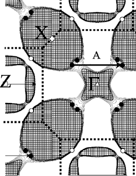
Figure 2: The cross section including the $\Gamma$ point of FS with the bct Brillouin zone for the 17th band. A solid circle $\bullet$ and an open circle $\circ$ indicate the positions of point-node and the local minima, respectively. An open triangle $\triangle$, box $\Box$ and diamond $\Diamond$ indicate the $\Gamma$ point, $Z$ point, $X$ point, respectively.

IV.2 Angular Dependence of the Density of States in the Weak Magnetic Fields

Comparing with the FAD heat capacity and the AV thermal conductivity experiments, we calculate the density of states with the Doppler-shift method.Volovik Without impurity scattering (superclean limit), the quasiclassical Green function is written as

$$g(\mbox{\boldmath$r$},\hat{\mbox{\boldmath$p$}};{\rm i}\omega_{n})=\frac{\omega_{n}+{\rm i}\mbox{\boldmath$v$}_{\rm F}\cdot\mbox{\boldmath$v$}_{\rm s}}{\sqrt{(\omega_{n}+{\rm i}\mbox{\boldmath$v$}_{\rm F}\cdot\mbox{\boldmath$v$}_{\rm s})^{2}+|\Delta|^{2}}}.$$ (41)

Here, $\mbox{\boldmath$v$}_{\rm s}$ is the supercurrent velocity around a vortex. Therefore, the density of states at zero-energy $\nu(\epsilon=0)$ is written as

$$\nu(\epsilon=0,\phi)=\Bigl{\langle}{\rm Re}\frac{d(\phi)}{\sqrt{d^{2}(\phi)-|\Delta|^{2}}}\Bigl{\rangle}.$$ (42)

Here, $d(\phi)=|\mbox{\boldmath$v$}_{\rm F}\cdot\mbox{\boldmath$v$}_{\rm s}(\phi)|$, the bracket means averaging over both Fermi surface and unit cell of vortex lattice and $\phi$ is the angle between magnetic fields and the $a$ axis on the $a$-$b$ plane. Since the core states do not contribute to the specific heat in low magnetic fields, we neglect the spatial variation of the magnitude of the pair-potential and consider the spatial variation of the phase of the pair-potential around a vortex. Assuming $d\ll\Delta_{\infty}$, only the quasiparticles around nodes in momentum space contribute to the density of states. This assumption is appropriate in weak magnetic fields.

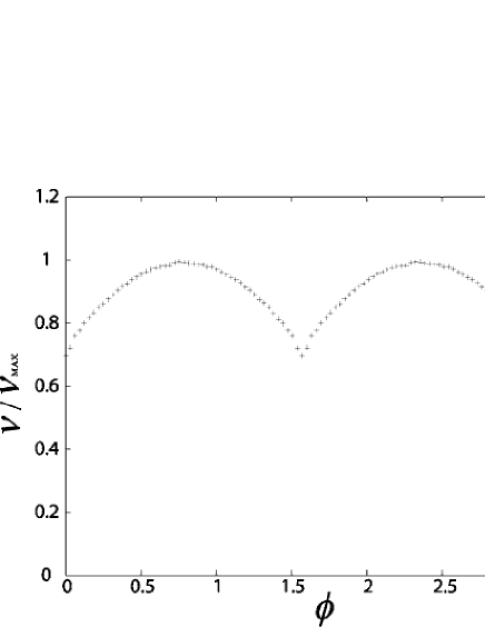
Figure 3: Angular dependence of specific heat $C_{\rm s}\propto\nu(\epsilon=0,\phi)$ with use of the band-structure of YNi₂B₂C. $\phi$ is the angle between magnetic field direction and the $a$ axis.

Figure 3 shows the angular dependence of specific heat $C_{\rm s}\propto\nu(\epsilon=0,\phi)$ calculated with use of the band-structure of YNi₂B₂C and the gap-structure consistent with the STM experiments (See Fig. 2). Here, the magnetic field is applied within the $a$-$b$ plane at an angle $\phi$ from the $a$ axis. It should be noted that narrow cusps appear at $\phi=0$ and $\phi=\pi/2$. This angular variation is consistent with the FAD heat capacity and the AV thermal transport experiments as shown in Fig. 2 in Ref. Park, and Fig. 2 in Ref. Izawa, , respectively. These angular variations can be explained by the fact that quasiparticles (QPs) around the gap-nodes in momentum space contribute to the DOS and QPs traveling parallel to the vortex do not contribute to the DOS (Note that QP with $\mbox{\boldmath$v$}_{\rm F}$ parallel to the vortex line gives no contribution in Eq. (42) because $\mbox{\boldmath$v$}_{s}$ is perpendicular to the vortex line and $d=|{\bm{v}}_{\rm F}\cdot{\bm{v}}_{s}|=0$ for such a QP.). In other words, the narrow cusps appear at the direction of the Fermi velocity of QPs at the gap-nodes. In the case of YNi₂B₂C, the direction of the Fermi velocity at $\bullet$ is parallel to the $\langle$ 100 $\rangle$.

IV.3 Density of States without Magnetic Fields

Comparing with the result of the STM/STS experiment in the absence of magnetic fields,Nakai we calculate the density of states in the absence of magnetic field in the bulk region. In Fig. 4, we show the DOS with use of the band-structure and the gap-structure. Here, we assume the smearing parameter $\delta=0.05\Delta_{\infty}$. Any singularities like that at $E=0.5\Delta_{\infty}$in the case of $s$+$g$ wave superconductivityMakiThal do not occur in our gap-structure. Our result is consistent with the density of states by the STM/STS experiment shown in Fig. 4(c) in Ref.Nakai, .

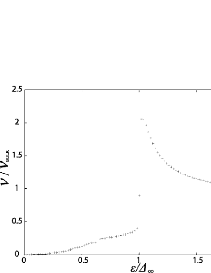
Figure 4: Quasiparticle density of states without magnetic fields. the smearing factor $\delta=0.05\Delta_{\infty}$.

IV.4 Angular Dependence of the LDOS patterns

One can obtain the three-dimensional information of the pairing symmetry from STM/STS experiments under the magnetic field with various directions. We have shown the LDOS patterns for the vortex parallel to the $b$ axis about $s$+$g$ wave superconductor in Fig. 14 in Ref. Nagai, . We calculate the LDOS patterns on the $a$-$b$ plane with various directions of magnetic fields, since the LDOS will be observed by the STM/STS experiments on the clean surface perpendicular to the crystal $c$ axis. As shown in Fig. 5, these LDOS patterns are different qualitatively. The four peaks in the LDOS patterns for the vortex parallel to the $c$ axis disappear in the LDOS patterns for the vortex tilting from the $c$ axis by angle $\theta=\pi/4$ within the $a$-$c$ plane as shown in Fig. 5(a). Only the two peaks remain in the LDOS pattern for the vortex tilting from the $a$ axis by angle $\phi=\pi/4$ and tilting from the $c$ axis by angle $\theta=\pi/4$ as shown in Fig. 5(b).

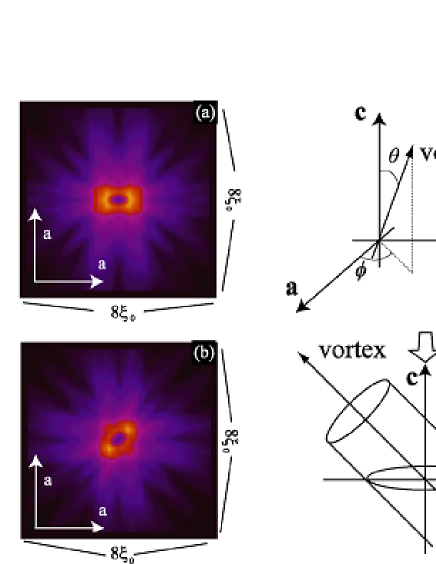
Figure 5: (Color Online) Distributions of the local density of states for the vortex tilting from the $a$ axis by angle $\theta$ and the $c$ axis by angle $\phi$.(a) $(\phi,\theta)=(0,\pi/4)$, (b) $(\phi,\theta)=(\pi/4,\pi/4)$. The smearing factor is $\delta=0.05\Delta_{\infty}$ and the energy is $\epsilon=0.3\Delta_{\infty}$. These LDOS patterns will be observed by the STM/STS experiments from the $c$ axis.

V Discussions

We considered the 17th band and neglect the 18th and 19th bands. By the angular resolved photo emission experiment,Baba the isotropic superconducting gap exists on the FS from 18th band and the FS from 19th band is not observed. Since the LDOS pattern from the isotropic superconducting gap is almost isotropic, the LDOS from 18th band does not contribute to the four peak structure of the STM/STS experiment. Comparing Fig. 1(c) with Fig. 1(f), the LDOS at the center by the theoretical calculation is quite smaller than that at a vortex center by the STM/STS experiments. Considering the FS from 18th band, it seems that this LDOS at a vortex center becomes large. Therefore, the calculations with use of the FSs from 17th and 18th bands are needed for quantitative comparison with STM/STS experiment.

The results of STM/STS experiments around a vortex can not be explained by the ‘two-gap model’ since the strong anisotropy of the gap-structure makes the four peak structure of this experiment. Two isotropic gaps make two isotropic LDOS patterns even if the highly anisotropic FS is considered. The LDOS patterns with the model of point-nodes and that with the two-gap model are qualitatively different in the zero energy region as shown in Fig. 1(d).

The previous analyses of the FAD heat capacity and the AV thermal transport experiments are insufficient since the isotropic FS is assumed, so that these analyses lead to the wrong conclusion that the gap function has point-nodes along the $a$ axis and $b$ axis. The information about nodes we obtain is the directions of the Fermi velocity at the nodes on the FS, since the Doppler-shift method is based on the fact that the energy has the term proportional to $\mbox{\boldmath$v_{\rm F}$}\cdot\mbox{\boldmath$v_{\rm s}$}$ as shown in Eq. 42. Therefore, these experiments suggest that the Fermi velocity at the nodes on the FS is parallel to the $a$ axis (the direction of nesting vectors). In the case of the anisotropic FS, the directions of the point-nodes are not found only from these experiments. In the only case of the isotropic FS, the directions of the point-nodes are parallel to the Fermi velocity at the nodes.

We have shown that the point-nodes in momentum space are at the ‘vector A’. These results suggest that the strong antiferromagnetic fluctuations suppress the superconducting order parameter at these points.MakiThal ; Kontani The reason why the point-nodes do not exist at the ‘the vector B’ is not clear yet. This is a future problem.

VI Conclusion

In conclusion, we calculated the LDOS patterns around a vortex core, the angular dependence of the DOS in weak magnetic field, the DOS in zero fields in the bulk region and the LDOS patterns for the vortex tilting from the crystal $c$ axis with use of the FS from 17th band obtained by the band-calculations, assuming various gap structures where positions of point-nodes are different. Comparing our theoretical calculations with the results of the STM/STS, the FAD heat capacity and the AV thermal transport experiments, we determined the gap-structure which is consistent with these experiments. The point-nodes are at ‘the vector A’, which is along $\langle 110\rangle$ as shown in Fig. 2. We also showed that the previous analyses of the FAD heat capacity and the AV thermal transport experiments are insufficient since the isotropic FS was assumed. Considering the anisotropic FS, we showed the most suitable gap structure. This gap structure is consistent with the results of the FAD heat capacity, the AV thermal transport, the density of states without magnetic fields by the STM and the local density of states around a vortex core by the STM. We hope that our results will be tested by the STM/STS experiments with the rotation of the magnetic fields.

References

- (1) R. J. Cava, H. Takagi, H. W. Zandbergen, J. J. Krajewski, W. F. Peck Jr., T. Siegrist, B. Batlogg, R. B. van Dover, R. J. Felder, K. Mizuhashi, J. O. Lee, H. Eisaki and S. Uchida, Nature (London) 367, 252 (1994).
- (2) D. D. Lawrie, J. P. Frank, Physica C 245, 159 (1995).
- (3) K. O. Cheon, I. R. Fisher, P. C. Canfield, Physica C 312, 35 (1999).
- (4) K-H. Muller and V. N. Narozhnyi, Rep. Prog. Phys. 64, 943 (2001).
- (5) K. Maki, P. Thalmeier and H. Won, Phys. Rev. B 65, 140502(R) (2002).
- (6) T. Park, M. B. Salamon, E. M. Choi, H. J. Kim and S. I. Lee, Phys. Rev. Lett. 90, 177001 (2003).
- (7) K. Izawa, K. Kamata, Y. Nakajima, Y. Matsuda, T. Watanabe, M. Nohara, H. Takagi, P. Thalmeier and K. Maki, Phys. Rev. Lett. 89, 137006 (2002).
- (8) J. I. Lee, T. S. Zhao, I. G. Kim, B. I. Min and S. J. Youn, Phys. Rev. B 50, 4030 (1994).
- (9) D. J. Singh, Solid State Commun. 96, 899 (1996).
- (10) K. Yamauchi, H. Katayama-Yoshida, A. Yanase and H. Harima, Physica C 412-414, 225 (2004).
- (11) H. Nishimori, K. Uchiyama, S. Kaneko, A. Tokura, H. Takeya, K. Hirata and N. Nishida, J. Phys. Soc. Jpn. 73, 3247 (2004).
- (12) Y. Nagai, U, Ueno, Y. Kato and N. Hayashi, J. Phys. Soc. Jpn. 75, 104701 (2006).
- (13) H. F. Hess, R. B. Robinson and J. V. Waszczak, Phys. Rev. Lett. 64, 2711 (1990).
- (14) F. Gygi and M. Schlüter, Phys. Rev. B 43, 7609 (1991).
- (15) N. Hayashi, M. Ichioka and K. Machida, Phys. Rev. B 56, 9052 (1997).
- (16) N. Schopohl and K. Maki, Phys. Rev. B 52, 490 (1995).
- (17) M. Ichioka, N. Hayashi, N. Enomoto and K. Machida, Phys. Rev. B. 53, 15316 (1996).
- (18) C. Caroli, P. G. de Gennes and J. Matricon, Phys. Lett. 9, 307 (1964).
- (19) L. Kramer and W. Pesch, Z. Phys. 269, 59 (1974).
- (20) Y. Nagai, Y. Kato and N. Hayashi, J. Phys. Soc. Jpn. 75, 043706 (2006).
- (21) H. Harima, O. Sakai, T. Kasuya and A. Yanase, Solid State Commun. 66, 603 (1988).
- (22) T. Ebihara, Y. Inada, M. Murakawa, S. Uji, C. Terakura, T. Terashima, E. Yamamoto, Y. Haga, Y. Onuki and H. Harima, J. Phys. Soc. Jpn. 69, 895 (2000).
- (23) H. Harima and K. Takegahara, J. Magn. Magn. Matter. 272-276, 475 (2004).
- (24) G. E. Volovik, Pis’ma Zh. Eksp. Teor. Fiz. 58, 457 (1993)[JETP Lett. 58, 469 (1993)].
- (25) M. Sigrist and K. Ueda, Rev. Mod. Phys. 63, 239 (1991).
- (26) A. I. Larkin and Yu. N. Ovchinnikov, Zh. ksp. Teor. Fiz. 55, 2262 (1968), [Sov. Phys. JETP 28, 1200 (1969)].
- (27) G. Eilenberger, Z. Phys. 214, 195 (1968).
- (28) J. W. Serene and D. Rainer, Phys. Rep. 101, 221 (1983).
- (29) M. Eschrig, Phys. Rev. B 61, 9061 (2000).
- (30) A. L. Shelankov, J. Low Temp. Phys. 60, 29 (1985).
- (31) N. Nakai, P. Miranovic, M. Ichioka, H. F. Hess, K. Uchiyama, H. Nishimori, S. Kaneko, N. Nishida and K. Machida, Phys. Rev. Lett. 97, 147001 (2006).
- (32) T. Baba, Doctor thesis, University of Tokyo, 2007.
- (33) H. Kontani, Phys. Rev. B 70, 054507 (2004).