Solar transition region features observed with Hinode/EIS

Abstract

Two types of solar active region feature prominent at transition region temperatures are identified in Hinode/EIS data of AR 10938 taken on 2007 January 20. The footpoints of 1 MK TRACE loops are shown to emit strongly in emission lines formed at $\log~{}T=5.4$–5.8, allowing the temperature increase along the footpoints to be clearly seen. A density diagnostic of Mg vii yields the density in the footpoints, with one loop showing a decrease from $3\times 10^{9}$ cm^-3 at the base to $1.5\times 10^{9}$ cm^-3 at a projected height of 20 Mm. The second feature is a compact active region transition region brightening which is particularly intense in O v emission ($\log~{}T=5.4$) but also has a signature at temperatures up to $\log~{}T=6.3$. The Mg vii diagnostic gives a density of $4\times 10^{10}$ cm^-3, and emission lines of Mg vi and Mg vii show line profiles broadened by 50 km s^-1 and wings extending beyond $\pm 200$ km s^-1. Continuum emission in the short wavelength band is also found to be enhanced, and is suggested to be free-bound emission from recombination onto He⁺.

1 Introduction

The Extreme ultraviolet Imaging Spectrometer (EIS) instrument on Hinode (Culhane et al., 2007; Kosugi et al., 2007) covers the two wavelength bands 170–211 and 246–292 Å that are dominated by coronal emission lines mainly from the iron ions. The majority of strong transition region lines in the solar spectrum are found at longer UV wavelengths, and all of the transition region lines found in the EIS bands are weak in normal conditions. Young (2007) however identified two types of active region features that were found from SOHO/CDS observations to yield significantly enhanced transition region emission lines: coronal loop footpoints and active region blinkers. He suggested that in such events the weak EIS lines would become significant, and so yield useful science. An EIS observation from 2007 January 20 is presented here that displays both types of active region feature identified by Young (2007) and demonstrates the value of including transition region lines in EIS studies.

2 Data

Active region AR 10938 crossed the solar disk during 2007 January 12–24. It was a well developed active region showing large cool loop structures visible in the TRACE 171 channel (Fig. 1, left panel), and a more compact high temperature core visible in Hinode/XRT images (Fig. 1, right panel) During the period January 18–23 the EIS observing study PRY_loop_footpoints was run a number of times at the footpoint regions of the loop system. This study uses the 2 slit to raster over an area of 100$\times$216 with 30 second exposure times, giving a total duration of 26 minutes. The 2 slit was used to both increase the counts for weak lines, and allow a larger spatial area to be covered more rapidly; the disadvantages are a degradation of the spatial (in the X-direction) and spectral resolution over the 1 slit. Due to on board data storage restrictions, only a fraction of the total EIS wavelength range could be downloaded, and so 20 wavelength windows were chosen to observe the transition region lines as well as a number of coronal lines. The list of the transition region lines (defined as emission lines whose temperature of maximum ionization, $T_{\rm max}$, is below $\log\,T=5.8$) is given in Table 1. Further discussion of useful emission transition region lines observed with EIS is given in Young et al. (2007).

Table 1: Transition region emission lines observed with the PRY_loop_footpoints EIS study.

Ion	Wavelength/Å	Transition	Log $T_{\rm max}$/K
O v	192.8a	2s2p ${}^{3}P^{\rm o}_{0,1}$ – 2s3d 3D1,2	5.4
O v	192.9b	2s2p ${}^{3}P^{\rm o}_{2}$ – 2s3d 3D3,2	5.4
Mg v	276.58	2s22p4 1D2 – 2s2p5 ${}^{1}P^{\rm o}_{1}$	5.4
Fe viii	185.12	3p63d 2D5/2 – 3p53d2 ${}^{1}P^{\rm o}_{1}$	5.6
Mg vi	268.99	2s22p3 ${}^{2}D^{\rm o}_{3/2}$ – 2s2p4 2P1/2	5.6
	270.40	2s22p3 ${}^{2}D^{\rm o}_{3/2,5/2}$ – 2s2p4 2P3/2	5.7
Mg vii	278.39	2s22p2 3P2 – 2s2p3 ${}^{3}S^{\rm o}_{1}$	5.8
	280.75	2s22p2 1D2 – 2s2p3 ${}^{1}P^{\rm o}_{1}$	5.8
Si vii	275.35	2s22p4 3P2 – 2s2p5 ${}^{3}P^{\rm o}_{2}$	5.8
a comprises three lines with wavelengths 192.750, 192.797, 192.801 Å.
b comprises two lines with wavelengths 192.904 and 192.911 Å.

Raster images for a number of the emission lines are shown in Fig. 2. The two EIS wavelength bands are imaged onto different CCDs and there is a spatial offset in the Solar-Y direction between the CCDs that varies with wavelength and ranges from 16 to 20 pixels depending on the wavelengths being compared. A fixed offset of 17 pixels has been applied to the images in Fig. 2. In addition, when comparing raster images from the two CCDs, there is a spatial offset in the solar-X direction of around 2 arcsec. The images have also been corrected for this effect.

The data have been calibrated to yield intensities in units of erg cm^-2 s^-1 sr^-1 at each pixel in the data-set. The dark current and CCD pedestal were removed by subtracting the median value of the darkest 2 % pixels in each wavelength window. Cosmic rays and CCD hot pixels were removed using the IDL routine NEW_SPIKE. The conversions from data numbers to photons and on to calibrated intensites were performed using data contained in the EIS directory of the Solarsoft IDL distribution.

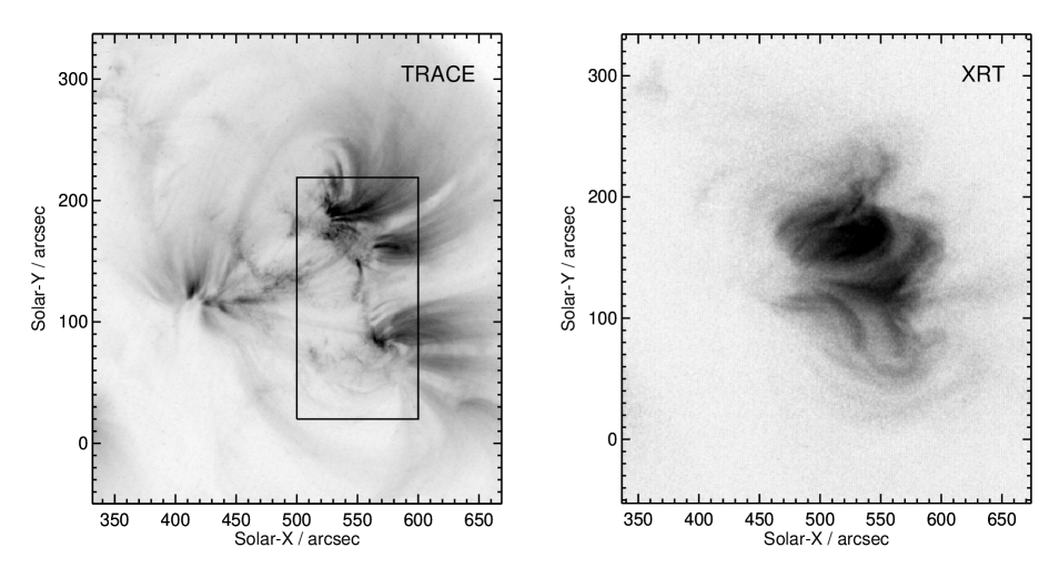
Figure 1: The left-hand panel shows a TRACE 171 filter image taken at 22:40 UT. The approximate location of the EIS raster is indicated by a black box. The right-hand panel shows a XRT image taken with the Al-Poly filter at 22:36 UT. For both images dark areas are bright in intensity.

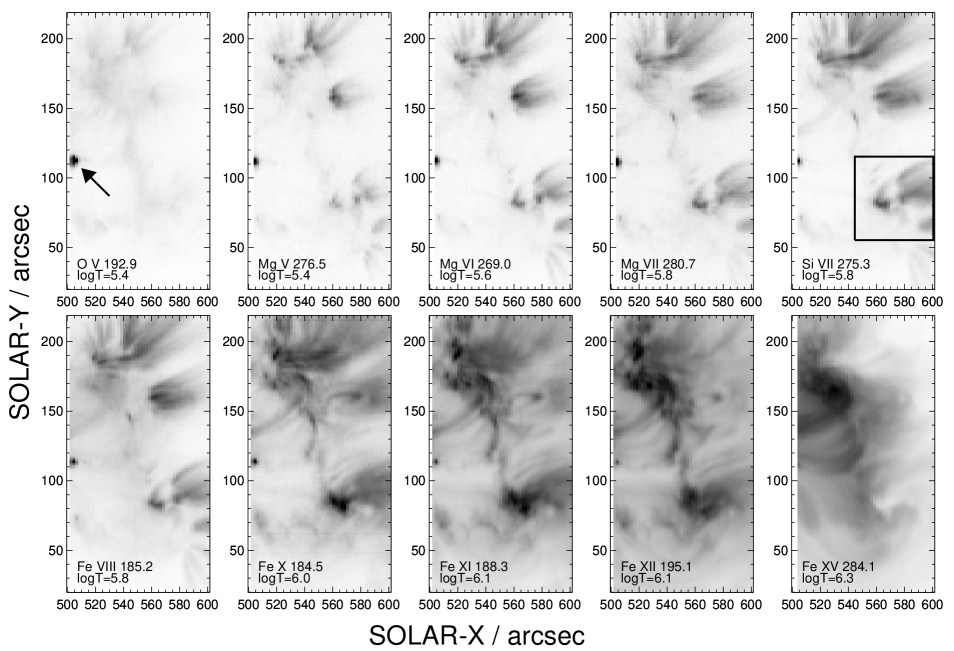
Figure 2: EIS raster images in ten different emission lines for the spatial region indicated in the TRACE image of Fig. 1. The loop footpoints are most clearly seen in Mg v–vii, Si vii and Fe viii. The box on the Si vii image indicates the region shown in Fig. 3, while the arrow in the O v image points to the location of the ARTRB.

3 Loop footpoints

Fig. 2 shows a number of ‘clumps’ of loop footpoints that can be readily identified with the loops in the TRACE 171 image (Fig. 1). The spectroscopic properties of such loops have been studied previously by Del Zanna (2003) and Del Zanna & Mason (2003) using SOHO/CDS spectra. In particular, there is a steep temperature increase at the loop base, leading to transition region lines being formed in a small spatial area at the footpoint of the loop. The main body of the loop is at temperatures of around 1 MK and thus strongly emits in the Fe ix $\lambda$171.1 and Fe x $\lambda$174.5 emission lines that contribute to the TRACE 171 passband. The Mg vii $\lambda$319.0/$\lambda$367.7 density diagnostic yielded densities of $\approx$ $2\times 10^{9}$ cm^-3.

Although EIS lacks the strong transition region lines (such as Ne vi $\lambda$562.8, O v $\lambda$629.7) observed by SOHO/CDS, the images in Fig. 2 clearly demonstrate that the footpoints of the 1 MK loops can be identified in the EIS data. In particular, enhanced emission at the base of the loops can be seen in Mg v, Mg vi and, to a lesser extent, O v. A comparison from spectra in and outside of the footpoint regions is shown in Fig. 4, demonstrating the strong enhancement of the cool lines. Generally the cool Mg emission can be identified to extend for a significant length along the loops (10–50 arcsec). We demonstrate below how the EIS spectra can be used to derive temperature, density and filling factor information about these loops.

3.1 Temperature analysis

A simply visual inspection of the loop footpoint images in Fig. 2 shows that the Fe viii $\lambda$185.21 structures look very similar to Si vii $\lambda$275.35 structures. This is at odds with the temperatures of maxium ionization given in Table 1 that are derived from the Mazzotta et al. (1998) ion balance calculations. The ionization and recombination rates are expected to be considerably more uncertain for Fe⁷⁺ than those for Si⁶⁺ given its more complex atomic structure. A conclusion from the EIS images is thus that Fe viii is actually principally formed at a temperature of $\log\,T=5.8$. This will have a knock-on effect for Fe ix which also must be formed at a higher temperature than given by Mazzotta et al. (1998).

The different appearance of the loop footpoint regions in the Mg v, Mg vi and Si vii lines clearly demonstrates that the loops are not isothermal in the lowest $\approx 10$ Mm of the loop. We defer to a later paper a discussion of whether the loops are actually multithermal in this region (i.e., a range of temperatures applies at a given point in the loop), or whether the temperature is simply decreasing towards the footpoints. Del Zanna (2003) inferred the latter from his analysis of SOHO/CDS spectra.

Two weak footpoints are highlighted by two arrows in the Mg vi image of Fig. 3. They show a different character to the other more extended footpoints in the image, being significantly more compact in Mg v–vii. Comparing the different images in Fig. 2 and also the TRACE image (Fig. 1), shows that these loops are hotter, emitting principally in Fe xii $\lambda$195.1 rather than Fe ix and Fe x.

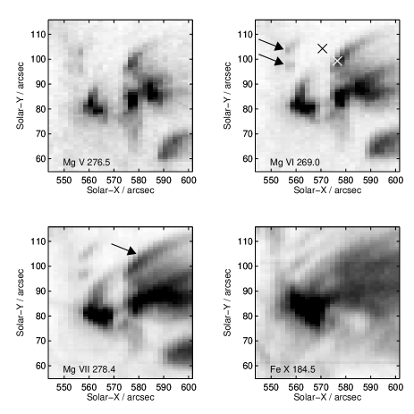
Figure 3: A close-up of the footpoint region indicated in the Si vii image of Fig. 2. Arrows point to two weak footpoints in the Mg vi image that are the compact footpoints of hot loops. The arrow in the Mg vii image points to the loop selected for density analysis. The two crosses on the Mg vi image indicate the spatial pixels from which the spectra shown in Fig. 4 were obtained.

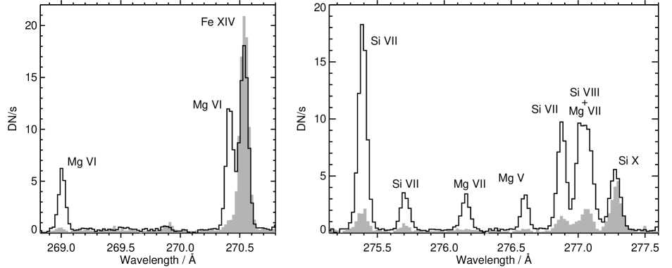
Figure 4: A comparison of spectra at the two pixels identified in Fig. 3. The spectrum from within the footpoint (white cross in Fig. 3) is identified with a solid line. The shaded spectrum is from a pixel outside of the footpoint (black cross in Fig. 3). The Y-axis shows the strength of the lines in data numbers (DN) per second.

3.2 Density analysis

The EIS long wavelength channel contains the Mg vii $\lambda$280.75/$\lambda$278.39 density diagnostic which is directly comparable to the $\lambda$319.0/$\lambda$367.7 diagnostic that is observed with SOHO/CDS (Young & Mason, 1997; Del Zanna, 2003). The diagnostic is sensitive to densities in the range $10^{8}$–$10^{11}$ cm^-3 (Fig. 5), but analysis is complicated by a blend of the $\lambda$278.39 line with Si vii $\lambda$278.44. A simultaneous two Gaussian fit to the feature is, however, able to resolve the two components if both are assumed to have the same width (this is a reasonable assumption since the two ions are formed at very similar temperatures). Tests of the validity of the two Gaussian fits have been confirmed with the current data-set by comparing the derived intensities with the Si vii $\lambda$275.35 and Mg vii $\lambda$276.14 lines. The Si vii $\lambda$278.44/$\lambda$275.35 and Mg vii $\lambda$276.14/$\lambda$278.39 ratios are branching ratios with fixed theoretical ratios of 0.32 and 0.20, respectively.

Figure 5: Theoretical variation of the Mg vii $\lambda$280.75/$\lambda$278.39 ratio with density. Produced using v.5.2 of the CHIANTI atomic database (Landi et al., 2006).

Fig. 6 shows the densities derived from the Mg vii diagnostic for a number of positions along the loop structure highlighted by an arrow in the Mg vii image of Fig. 3. Four to five pixels across the loop width (i.e., in the solar-Y direction) were averaged to derive the line intensities. An estimate of the background was made by summing a number of pixels in a low intensity region just to the north of the loop. There is a clear trend of decreasing density along the structure. The density estimates are in excellent agreement with those obtained by Del Zanna (2003) and Del Zanna & Mason (2003) demonstrating that such values are typical for 1 MK loops. The improved spatial resolution of EIS over CDS now means that the spatial variation of density in the footpoint regions can be accurately measured giving additional constraints on theoretical loop models.

By assuming an isothermal plasma whose temperature is the $T_{\rm max}$ of Mg vii it is possible to use the density measurements to estimate the column depth of the plasma in the loop. The atomic data from v5.2 of CHIANTI (Landi et al., 2006; Dere et al., 1997) were used together with the coronal abundances of Feldman et al. (1992) to derive column depths of 1.6–5.4 Mm (2.3–7.4). These values are comparable to the observed diameter of the loop (around 5–10) and thus suggest a filling factor of around unity.

Figure 6: Electron densities derived from the Mg vii $\lambda$280.75/$\lambda$278.39 density diagnostic.

4 Transition region brightening

The small intense brightening (heretoafter referred to as an ARTRB – active region transition region brightening) seen in the raster images (Fig. 2) was only present in one of the sequence of EIS rasters. However, the evolution of the event can be seen from TRACE images (Fig. 7) that demonstrate that it began at 22:42 UT and had faded completely by 23:49 UT. No TRACE data were available between 22:55 UT and 23:42 UT. The peak intensity occurred at 22:55 UT, corresponding closely to the time at which EIS scanned the region (22:57 UT). The brightening is very bright in the transition region at the temperature of O v ($\log\,T=5.4$) and the brightness decreases to higher temperatures, until it is barely discernible in Fe xv ($\log\,T=6.3$). The brightening is not apparent in co-temporal XRT images.

The density and temperature properties (discussed below) appear to be similar to those of impulsive events identified in EUV Skylab spectra by Widing (1982), and to an active region brightening seen in EUV spectra from SOHO/CDS by Young & Mason (1997), later termed active region blinkers and discussed further by Young (2004). There are also similarities in terms of intensity enhancement and line broadening to the bidirectional jet observed by Doyle et al. (2004) in TRACE and SOHO/SUMER data.

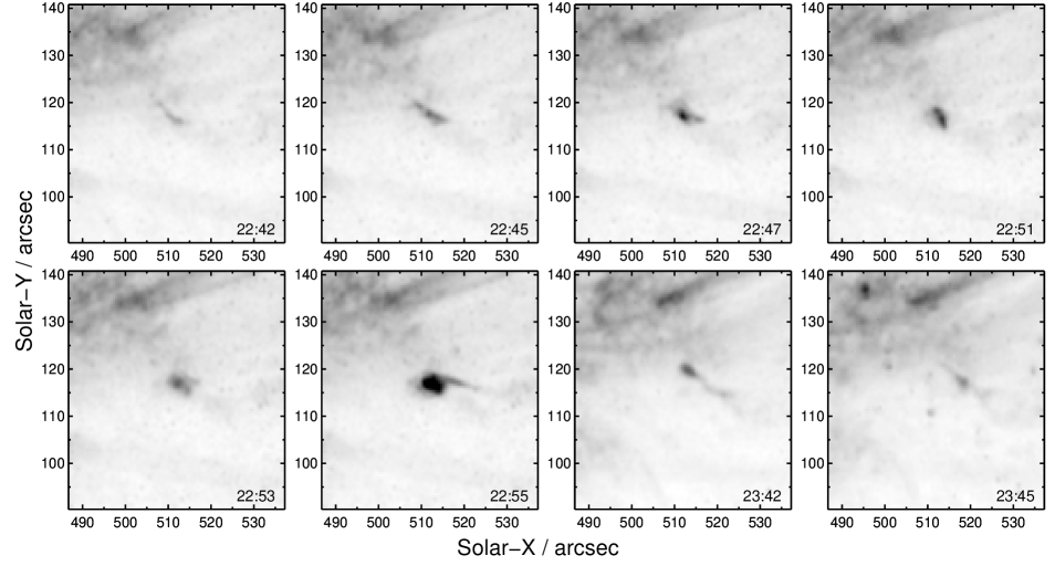
Figure 7: Evolution of the ARTRB as observed by TRACE in the 171 filter. No TRACE data were available between 22:55 and 23:42 UT. EIS observed the ARTRB at 22:57 UT.

4.1 Oxygen emission lines

A number of n=3 to 2 transitions of O iv–vi are found in the EIS wavebands (Young et al., 2007). They are mostly very weak but can be detected with the high spectral resolution and sensitivity of EIS. The O v 2s2p ${}^{3}P^{\rm o}_{J}$ – 2s3d ³D${}_{J^{\prime}}$ transitions are of particular interest as they lie close to Ca xvii 192.82 – an EIS core line that is observed in every EIS study. (This line is actually blended with Fe xi $\lambda$192.83 which dominates in most solar conditions.) The left-hand panel of Fig. 8 compares spectra of the ARTRB with a region outside of the ARTRB. The dashed line shows the normally dominant Fe xi line, while the solid line demonstrates the strong enhancement of O v $\lambda$192.9. The contribution of O v is complicated as there are actually five significant O v components and the CHIANTI prediction for the relative strengths is shown in the right panel of Fig. 8. It is thus seen that O v makes up around one half of the emission seen at 192.8 Å.

Figure 8: Left panel: a comparison of spectra in the vicinity of the Fe xi–Ca xvii–O v blend at 192.8–192.9 Å. The solid line is a spectrum from the ARTRB, while the dashed line is from a region to the north of the brightening showing the more typical appearance of the spectrum. Right panel: a synthetic spectrum generated with CHIANTI showing the five O v components (vertical lines) and the resulting spectral distribution (assuming Gaussian line profiles).

4.2 Line broadening

The brightening displays significantly broadened line profiles in the transition region, as demonstrated for Mg vi $\lambda$268.99 and Mg vii $\lambda$280.75 in Fig. 9. The cores of the lines are seen to be broadened by around 50 km s^-1 while the wings extend out beyond $\pm 200$ km s^-1. Given the strongly dynamic behaviour of the ARTRB in the TRACE movie, these features are most likely to be due to a superposition of high speed up- and down-flows in the structure.

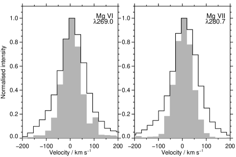
Figure 9: A comparison of emission line profiles for Mg vi $\lambda$269.0 (left-hand panel) and Mg vii $\lambda$280.7 (right-hand panel). The shaded feature gives the line profile averaged over a number of spatial pixels in one of the loop footpoints, the solid line gives the profile in the ARTRB.

4.3 Density

The Mg vii ratio used in the previous section yields a density of $\log\,N_{\rm e}$=$10.63^{+0.10}_{-0.09}$ for the ARTRB. Note that, because of the non-Gaussian profiles, it was necessary to use the Si vii $\lambda$275.35 line to estimate the Si vii contribution to Mg vii $\lambda$278.39. This high density is consistent with the high densities measured by Widing (1982), Young & Mason (1997) and Young (2004) for the transition region events they studied using Skylab and SOHO/CDS spectra, respectively.

4.4 Continuum emission

Another feature demonstrated by this small brightening is enhanced continuum emission in the short wavelength band (Fig. 10). The continuum level has been estimated from regions apparently free of emission lines, however Fig. 10 suggests that some of the regions chosen are affected by emission lines. The continuum is probably due to recombination onto H-like helium. The photoionization edge of He⁺ is at 227.8 Å, thus explaining why there is little continuum enhancement in the long wavelength band. Note that the continuum level appears to rise at the longest wavelengths in the 246–292 Å band. This is probably the short wavelength wing of He ii $\lambda$304, given the significant broadening of other cool lines in the EIS spectrum (Fig. 9).

Figure 10: Plot showing continuum emission for the ARTRB in the two EIS wavelength bands. The continuum level has been estimated from spectral regions believed to be free from emission lines.

4.5 Time evolution

The short lifetime of this ARTRB (as judged from the TRACE data) means that high cadence (at most a few minutes between rasters) EIS rasters are required to study such events in detail. EIS has the capability of automatically switching to a new study if a threshold intensity is reached in a specified emission line, and this will be a valuable tool for studying such short-lived features. EIS slot movies are also an alternative as the small spatial scale of the events should limit any spatial–spectral ambiguity introduced by using a wide slit. XRT data would appear to be of limited value due to the low temperature of the events, but SOT data will be extremely important for relating the ARTRBs to the magnetic field and photospheric/chromospheric plasma. A cursory glance of Ca ii images reveals that the ARTRB here is located at the edge of a plage region and is bright in Ca ii.

5 Conclusions

The EIS active region data-set shown here shows two types of structure that yield strongly enhanced transition region emission lines. Footpoints of large active region loops that are most characteristically seen in TRACE 171 filter images can clearly be seen in emission lines of Mg v–vii, Si vii and Fe viii – ions formed at temperatures $\log\,T=5.4$–5.8. The density in these footpoint regions can be accurately measured using the Mg vii $\lambda$280.75/$\lambda$278.39 ratio, and a fall-off in density from $3\times 10^{9}$ to $1.5\times 10^{9}$ cm^-3 from the base of a loop to a (projected) height of 20 Mm is found here.

A strong active region transition region brightening (ARTRB) is also seen in the data-set and demonstrates very strong emission in O v $\lambda$192.9. The ARTRB shows broadened emission line profiles and extended wings. The Mg vii $\lambda$280.75/$\lambda$278.39 yields a density of $4\times 10^{10}$ cm^-3. The brightening is short-lived, but co-spatial TRACE images demonstrate a highly dynamic, small loop-like feature with a lifetime of around 60 minutes.

The value of including transition region lines in EIS studies has been demonstrated here, and observers are recommended to include one or more of the emission lines listed in Table 1 when designing EIS studies.

Hinode is a Japanese mission developed and launched by ISAS/JAXA, with NAOJ as domestic partner and NASA and STFC (UK) as international partners. It is operated by these agencies in co-operation with ESA and NSC (Norway). The authors thank D. Bewsher for useful comments on the manuscript. G. Del Zanna thanks the hospitality of DAMTP, University of Cambridge.

References

- Culhane et al. (2007) Culhane, J. L., Harra, L. K., James, A. M., et al. 2007, Solar Physics, in press
- Del Zanna (2003) Del Zanna, G. 2003, A&A, 406, L5
- Del Zanna & Mason (2003) Del Zanna, G., & Mason, H. E. 2003, A&A, 406, 1089
- Dere et al. (1997) Dere, K. P., Landi, E., Mason, H. E., Monsignori-Fossi, B. F., & Young, P. R. 1997, A&AS, 125, 149
- Doyle et al. (2004) Doyle, J. G., Madjarska, M. S., Dzifčáková, E., & Dammasch, I. E. 2004, Sol. Phys., 221, 51
- Feldman et al. (1992) Feldman, U., Mandelbaum, P., Seely, J. L., Doschek, G. A., & Gursky H. 1992, ApJS, 81, 387
- Kosugi et al. (2007) Kosugi, T., Matsuzaki, K., Sakao, T., et al. 2007, Solar Physics, submitted
- Landi et al. (2006) Landi, E., Del Zanna, G., Young, P. R., Dere, K. P., Mason, H. E., & Landini, M. 2006, ApJS, 162, 261
- Mazzotta et al. (1998) Mazzotta, P., Mazzitelli, G., Colafrancesco, S., & Vittorio, N. 1998, A&AS, 133, 403
- Widing (1982) Widing, K. G. 1982, ApJ, 258, 835
- Young & Mason (1997) Young, P. R., & Mason, H. E. 1997, Sol. Phys., 175, 523
- Young (2004) Young, P. R. 2004, in Proc. 13th SOHO Workshop, ESA SP-547, page257
- Young (2007) Young, P. R. 2007, in ASP Conf. Ser., 369, New Solar Physics with the Solar-B Mission, ed. K. Shibata, S. Nagata, & T. Sakurai (San Francisco: ASP), in press
- Young et al. (2007) Young, P. R., Del Zanna, G., Mason, H. E., et al. 2007, PASJ, this issue