Nonlinear turbulent magnetic diffusion and effective drift velocity of large-scale magnetic field in a two-dimensional magnetohydrodynamic turbulence

Abstract

We study a nonlinear quenching of turbulent magnetic diffusion and effective drift velocity of large-scale magnetic field in a developed two-dimensional MHD turbulence at large magnetic Reynolds numbers. We show that transport of the mean-square magnetic potential strongly changes quenching of turbulent magnetic diffusion. In particularly, the catastrophic quenching of turbulent magnetic diffusion does not occur for the large-scale magnetic fields $B\gg B_{\rm eq}/\sqrt{\rm Rm}$ when a divergence of the flux of the mean-square magnetic potential is not zero, where $B_{\rm eq}$ is the equipartition mean magnetic field determined by the turbulent kinetic energy and ${\rm Rm}$ is the magnetic Reynolds number. In this case the quenching of turbulent magnetic diffusion is independent of magnetic Reynolds number. The situation is similar to three-dimensional MHD turbulence at large magnetic Reynolds numbers whereby the catastrophic quenching of the $\alpha$ effect does not occur when a divergence of the flux of the small-scale magnetic helicity is not zero.

I Introduction

The magnetic fields of the Sun, solar type stars, galaxies and planets are believed to be generated by a dynamo process due to the simultaneous action of the $\alpha$ effect (the helical motions of turbulence) and differential rotation (see, e.g., M78 ; P79 ; KR80 ; ZRS83 ; RSS88 ; S89 ). The kinematic stage of the mean-field dynamo, i.e. the growth of a weak mean magnetic field with negligible effect on the turbulent flows, is well understood, while the nonlinear stage of dynamo evolution is a topic of intensive discussions (for reviews, see KU99 ; O03 ; BS05 ). The most contentious issue is the question of the equilibrium magnetic field strength at which dynamo action saturates. In particular, the problem of catastrophic quenching of the $\alpha$ effect in a developed three-dimensional magnetohydrodynamic (MHD) turbulence with large magnetic Reynolds numbers has been intensively discussed in astrophysics and magnetohydrodynamics during last years (see, e.g., CV91 ; VC92 ; GD94 ; CH96 ). The catastrophic quenching implies very strong reduction of the $\alpha$ effect during the growth of the mean magnetic field so that the dynamo generated magnetic field should be saturated at a very low level. However, this is in contradiction with observations of the magnetic fields of the Sun, stars and galaxies.

In a two-dimensional MHD turbulence with imposed large-scale magnetic field at large magnetic Reynolds numbers, the catastrophic quenching can occur for turbulent magnetic diffusion (see, e.g., CV91 ; DHK05 ). In particular, small-scale magnetic fluctuations strongly affect the large-scale magnetic field dynamics even for very weak mean fields. This causes a strong reduction of turbulent magnetic diffusion CV91 . This conclusion is based on Zeldovich theorem Z57 . In a two-dimensional MHD turbulence energy is transferred from large-scale stirring to small scales and dissipated due to an Alfvenized cascade, whereby eddy energy is converted to Alfven wave energy (see, e.g., I64 ; K65 ). The above discussed quenching is caused by the tendency of the mean magnetic field to Alfvenize the turbulence.

A principal difference between two-dimensional and three-dimensional MHD turbulence is related to different integral of motions for these kind of turbulence. In particular, square of total (small-scale and large-scale) magnetic potential is conserved in two-dimensional MHD turbulence, while total (small-scale and large-scale) magnetic helicity is conserved in three-dimensional MHD turbulence. The magnetic helicity and the $\alpha$ effect can be positive and negative, while the squared magnetic potential is only positive. A comprehensive comparison between two-dimensional and three-dimensional MHD turbulence has been performed in DHK05 ; DII05 .

It has been recently recognized BF00 ; KMRS00 that in three-dimensional MHD turbulence the catastrophic quenching of the $\alpha$ effect does not arises when a divergence of the flux of magnetic helicity is not zero (see also BS05 ; KKMR03 ; RKL06 ). In the present study we show that in a developed two-dimensional MHD turbulence with large magnetic Reynolds numbers ${\rm Rm}$, a non-zero divergence of the flux of the mean-square magnetic potential strongly changes a balance in the equation for these fluctuations and results in that the catastrophic quenching of turbulent magnetic diffusion does not occur for the magnetic fields $B\gg B_{\rm eq}/\sqrt{\rm Rm}$, where $B_{\rm eq}$ is the equipartition mean magnetic field determined by the turbulent kinetic energy.

This paper is organized as follows. In Sec. II we formulate the governing equations, the assumptions, the procedure of the derivations. In Sec. III we determine the nonlinear turbulent magnetic diffusion coefficients and the nonlinear drift velocities of the mean magnetic field in a developed two-dimensional MHD turbulence. Finally, we draw conclusions in Sec. IV. In Appendix A we perform the derivation of the nonlinear turbulent magnetic diffusion and the nonlinear drift velocities of the mean magnetic field and in Appendix B we present the nonlinear functions used in Sec. III and their asymptotic formulas.

II Governing equations and the procedure of derivation

Let us consider a developed two-dimensional MHD turbulence with large hydrodynamic and magnetic Reynolds numbers. We study nonlinear quenching of the turbulent magnetic diffusion and the effective drift velocity of the magnetic field. We use a mean field approach whereby the velocity, pressure and magnetic field are separated into the mean and fluctuating parts. In a two-dimensional MHD turbulence the mean magnetic field is ${\bf B}=\mbox{\boldmath$\nabla$}{\bf\times}[A(x,y)\,{\bf e}]$, where $A(x,y)$ is the mean magnetic potential and ${\bf e}$ is the unit vector perpendicular to the plane of the two-dimensional MHD turbulence, i.e., it is directed along $z$-axis. The equation for the evolution of the mean magnetic potential for an incompressible turbulent flow with a zero mean velocity reads:

$${\partial{A}\over\partial t}+{\rm div}\,\langle{\bf u}\,a\rangle=\eta\Delta{A}\;,$$ (1)

where ${\bf u}$ are the velocity fluctuations and $\eta$ is the magnetic diffusion caused by an electrical conductivity of a fluid. The mean electromotive force is ${\cal E}_{z}=\langle{\bf u}\times{\bf b}\rangle_{z}=-{\rm div}\,\mbox{\boldmath$\Gamma$}_{a}$, where the spatial flux of magnetic potential $\mbox{\boldmath$\Gamma$}_{a}=\langle{\bf u}\,a\rangle$ and magnetic fluctuations ${\bf b}=\mbox{\boldmath$\nabla$}{\bf\times}[a(x,y)\,{\bf e}]$ are described by the fluctuations of the magnetic potential $a(x,y)$. The mean electromotive force ${\cal E}_{z}({\bf B})$ in a two-dimensional MHD turbulence is given by:

$${\cal E}_{z}({\bf B}) = \{[{\bf V}^{\rm eff}({\bf B}){\bf\times}{\bf B}]_{i}-{\eta}_{ij}({\bf B})\,(\mbox{\boldmath$\nabla$}{\bf\times}{\bf B})_{j}\}\,e_{i}\;,$$ (2)

where the nonlinear turbulent magnetic diffusion ${\eta}_{ij}({\bf B})$ and the nonlinear effective drift velocity ${\bf V}^{\rm eff}({\bf B})$ of the mean magnetic field are determined in Sec. III.

In order to derive equations for the nonlinear turbulent magnetic diffusion and the nonlinear effective drift velocity of the mean magnetic field in a two-dimensional MHD turbulence we use a procedure outlined below (see Appendix A for details). This procedure is similar to that used in RK04 for a study of a three-dimensional MHD turbulence. We use equations for fluctuations of velocity and magnetic field

$${\partial{\bf u}(t,{\bf x})\over\partial t} = -{\mbox{\boldmath$\nabla$}p\over\rho}+{1\over\mu\,\rho}[({\bf b}\cdot\mbox{\boldmath$\nabla$}){\bf B}+({\bf B}\cdot\mbox{\boldmath$\nabla$}){\bf b}]$$ (3)

$$+{\bf u}^{N}+{\bf F}\,,$$

$${\partial{\bf b}(t,{\bf x})\over\partial t} = ({\bf B}\cdot\mbox{\boldmath$\nabla$}){\bf u}-({\bf u}\cdot\mbox{\boldmath$\nabla$}){\bf B}+{\bf b}^{N}\,,$$ (4)

where $\rho$ is the fluid density, ${\bf F}$ is a random external stirring force, ${\bf u}^{N}$ and ${\bf b}^{N}$ are the nonlinear terms which include the molecular dissipative terms, $p$ are the fluctuations of total (hydrodynamic and magnetic) pressure. Hereafter we omit the magnetic permeability of the fluid $\mu$ and include $\mu^{-1/2}$ in the definition of magnetic field, we also omit the density $\rho$ of incompressible fluid and include $\rho^{1/2}$ in the definition of velocity field. We rewrite Eqs. (3) and (4) in a Fourier space and derive equations for the two-point second-order correlation functions of the velocity fluctuations $\langle u_{i}\,u_{j}\rangle$, the magnetic fluctuations $\langle b_{i}\,b_{j}\rangle$ and the cross-helicity $\langle b_{i}\,u_{j}\rangle$. The equations for these correlation functions are given by Eqs. (16)-(LABEL:B8) in Appendix A.

The second-moment equations include the first-order spatial differential operators $\hat{\cal N}$ applied to the third-order moments $M^{(III)}$. A problem arises how to close the system, i.e., how to express the set of the third-order terms $\hat{\cal N}M^{(III)}$ through the lower moments $M^{(II)}$ (see, e.g., O70 ; MY75 ; Mc90 ). We use the spectral $\tau$ approximation which postulates that the deviations of the third-moment terms, $\hat{\cal N}M^{(III)}({\bf k})$, from the contributions to these terms afforded by the background turbulence, $\hat{\cal N}M^{(III,0)}({\bf k})$, are expressed through the similar deviations of the second moments, $M^{(II)}({\bf k})-M^{(II,0)}({\bf k})$:

$$\hat{\cal N}M^{(III)}({\bf k}) - \hat{\cal N}M^{(III,0)}({\bf k})$$ (5)

$$= -\,{1\over\tau(k)}\,[M^{(II)}({\bf k})-M^{(II,0)}({\bf k})]\;,$$

(see, e.g., O70 ; PFL76 ; KRR90 ; KMR96 ; RK04 ), where $\tau(k)$ is the scale-dependent relaxation time, which can be identified with the correlation time of the turbulent velocity field, and the quantities with the superscript $(0)$ correspond to the background turbulence. A justification of the $\tau$ approximation for different situations has been performed in numerical simulations and analytical studies in BS05 ; BF02 ; FB02 ; BK04 ; BSM05 ; SSB07 .

Next, we split all second-order correlation functions, $M^{(II)}$, into symmetric and antisymmetric parts with respect to the wave vector ${\bf k}$. We assume that the characteristic time of variation of the mean magnetic field ${\bf B}$ is substantially larger than the correlation time $\tau(k)$ for all turbulence scales. This allows us to get a stationary solution for the equations for the second-order moments, $M^{(II)}$. We use a model of the background anisotropic and inhomogeneous two-dimensional MHD turbulence determined by Eqs. (31)-(32) in Appendix A.

In this study we consider an intermediate nonlinearity which implies that the mean magnetic field is not enough strong in order to affect the correlation time of turbulent velocity field. The theory for a very strong mean magnetic field can be modified after taking into account a dependence of the correlation time of the turbulent velocity field on the mean magnetic field.

Using the solution of the derived second-moment equations, we determine the mean electromotive force, ${\cal E}_{i}=\varepsilon_{imn}\,\int\langle b_{n}\,u_{m}\rangle_{\bf k}\,{\rm d}{\bf k}$ (see Appendix A for details), where $\varepsilon_{ijk}$ is the fully antisymmetric Levi-Civita tensor. This procedure allows us to determine the nonlinear turbulent magnetic diffusion and the nonlinear effective drift velocity of the mean magnetic field in a two-dimensional MHD turbulence.

III Turbulent transport coefficients

The derivation outlined in Sec. II yields the nonlinear turbulent magnetic diffusion of the mean magnetic field. In particular, in order to determine the nonlinear turbulent magnetic diffusion ${\eta}_{ij}({\bf B})$ we use an identity: $\eta_{ij}=(\varepsilon_{ikp}b_{jkp}+\varepsilon_{jkp}b_{ikp})/4$, where the tensor $b_{ijk}$ is determined by Eq. (34) in Appendix A. The nonlinear turbulent magnetic diffusion coefficient along the mean magnetic field, $\eta_{{}_{B}}$, and the cross-field turbulent magnetic diffusion coefficient, $\eta_{{}_{\perp}}$, are given by:

$$\eta_{{}_{B}} = \tau_{0}\,[\langle{\bf u}^{2}\rangle^{(0)}-\langle{\bf b}^{2}\rangle^{(0)}]\,\Psi_{1}(\beta)\;,$$ (6)

$$\eta_{{}_{\perp}} = \tau_{0}\,[\langle{\bf u}^{2}\rangle^{(0)}-\langle{\bf b}^{2}\rangle^{(0)}]\,\Psi(\beta)\;,$$ (7)

where $\tau_{0}=l_{0}/u_{0}$ and $u_{0}=\sqrt{\langle{\bf u}^{2}\rangle^{(0)}}$ is the characteristic turbulent velocity in the maximum scale of turbulent motions $l_{0}$. The quantities with the superscript $(0)$ correspond to the background turbulence. The functions $\Psi(\beta)$, $\,\Psi_{1}(\beta)$ and their asymptotic formulas are given in Appendix B, $\beta=4\,(B/B_{\rm eq})$ and $B_{\rm eq}=\sqrt{\langle{\bf u}^{2}\rangle^{(0)}}$ is the equipartition field. More general equations for $\eta_{{}_{B}}$ and $\eta_{{}_{\perp}}$ in the case of an anisotropic background turbulence are given by Eqs. (LABEL:B36) and (36) in Appendix A. It follows from Eqs. (6) and (7) that in the case of Alfvenic equipartition, $\langle{\bf u}^{2}\rangle^{(0)}=\langle{\bf b}^{2}\rangle^{(0)}$, the nonlinear turbulent magnetic diffusion vanishes.

The nonlinear turbulent magnetic diffusion depends on a flux of mean-square magnetic potential. This flux can change properties of the quenching of the cross-field turbulent magnetic diffusion. Indeed, let us determine the parameter $\epsilon=\langle{\bf b}^{2}\rangle^{(0)}/\langle{\bf u}^{2}\rangle^{(0)}$ using budget equation for the evolution of the mean-square magnetic potential $\langle a^{2}\rangle$:

$${\partial\langle a^{2}\rangle\over\partial t}+{\rm div}\,{\bf F}^{A}=2\eta_{{}_{\perp}}{\bf B}^{2}-2\eta\langle{\bf b}^{2}\rangle\;,$$ (8)

where the flux ${\bf F}^{A}=\langle{\bf u}\,a^{2}\rangle-\eta\mbox{\boldmath$\nabla$}\langle a^{2}\rangle$ determines the transport of $\langle a^{2}\rangle$. The first term $2\eta_{{}_{\perp}}{\bf B}^{2}$ in the right hand side of Eq. (8) describes a production of the mean-square magnetic potential $\langle a^{2}\rangle$, while the term $-2\eta\langle{\bf b}^{2}\rangle$ determines the resistive dissipation of $\langle a^{2}\rangle$. In the absence of the flux of the mean-square magnetic potential, ${\bf F}^{A}=0$, Eq. (8) implies the catastrophic quenching of the cross-field turbulent magnetic diffusion. In particular, in a steady-state Eq. (8) reads $\eta_{{}_{\perp}}=\eta\,\langle{\bf b}^{2}\rangle/{\bf B}^{2}$. Since the magnetic energy is less than the kinetic energy, $\langle{\bf b}^{2}\rangle<\langle{\bf u}^{2}\rangle^{(0)}$, we get

$${\eta_{{}_{\perp}}\over\eta_{{}_{T}}}<{1\over{\rm Rm}\,(B/B_{\rm eq})^{2}}\;,$$ (9)

where $\eta_{{}_{T}}=l_{0}\,u_{0}/2$ and ${\rm Rm}=u_{0}\,l_{0}/\eta$ is the magnetic Reynolds number. This estimate implies a strong quenching of the cross-field turbulent magnetic diffusion with increasing ${\rm Rm}\,(B/B_{\rm eq})^{2}$ due to Alfvenization of turbulence by tangling of a weak mean magnetic field by velocity fluctuations DHK05 .

Situation is drastically changed when ${\rm div}\,{\bf F}^{A}\not=0$. Indeed, Eq. (8) is not closed because it depends on the magnetic energy $\langle{\bf b}^{2}\rangle$. The energy of magnetic fluctuations $\langle{\bf b}^{2}\rangle$ can be determined in the same way as we derived the cross-helicity tensor. In particular, $\langle{\bf b}^{2}\rangle$ is obtained from Eq. (LABEL:B24) given in Appendix A, after the integration in ${\bf k}$-space. The result is given by

$$\langle{\bf b}^{2}\rangle = {1\over 2}\Big{[}\langle{\bf u}^{2}\rangle^{(0)}[1-\phi(\beta)]+\langle{\bf b}^{2}\rangle^{(0)}[1+\phi(\beta)]\Big{]}\;,$$

(10)

where the function $\phi(\beta)$ and its asymptotic formulas are given in Appendix B. More general equation for $\langle{\bf b}^{2}\rangle$ for anisotropic background turbulence is given by Eq. (37) in Appendix A.

Equation (8) allows us to determine the energy of magnetic fluctuations of the background turbulence self-consistently. In particular, combining Eq. (10) with the steady-state solution of Eq. (8) we determine the parameter $\epsilon=\langle{\bf b}^{2}\rangle^{(0)}/\langle{\bf u}^{2}\rangle^{(0)}$ [see, e.g., Eq. (38) in Appendix A for anisotropic background turbulence]. When $B\gg B_{\rm eq}/\sqrt{\rm Rm}$, the parameter $\epsilon$ is given by

$$\epsilon=1-{{\rm div}\,{\bf F}^{A}\over 4\eta_{{}_{T}}B^{2}\Psi(\beta)}\;.$$ (11)

Therefore, Eqs. (6), (7) and (11) yield the nonlinear turbulent magnetic diffusion in two directions:

$$\eta_{{}_{B}} = {{\rm div}\,{\bf F}^{A}\over 2B^{2}}\,\biggl{(}{\Psi_{1}(\beta)\over\Psi(\beta)}\biggr{)}\;,$$ (12)

$$\eta_{{}_{\perp}} = {{\rm div}\,{\bf F}^{A}\over 2B^{2}}\;.$$ (13)

where $\eta_{{}_{B}}$ is the nonlinear turbulent magnetic diffusion along the mean magnetic field and $\eta_{{}_{\perp}}$ is the cross-field nonlinear turbulent magnetic diffusion. Remarkably, Eq. (13) can be obtained directly from Eq. (8) written in a steady-state if we neglect the resistive dissipation term $-2\eta\langle{\bf b}^{2}\rangle$ in the right hand side of Eq. (8).

In order to determine the parameter $\epsilon$ we use the steady-state solution of Eq. (8). However, the steady-state solution of this equation exists not for all values of the mean magnetic field. Indeed, let us plot in Fig. 1 the function $\Psi(\beta)$ for the exponent of the energy spectrum of the background turbulence $q=5/3$. At $B\to 0.18\,B_{\rm eq}$ the function $\Psi(\beta)$ tends to zero (see Fig. 1). In the range $B\geq 0.18\,B_{\rm eq}$ the steady-state solution of Eq. (8) does not exist. The turbulent magnetic diffusion should be positive, which implies that ${\rm div}\,{\bf F}^{A}>0$. Therefore, when ${\rm div}\,{\bf F}^{A}<0$ there is no steady-state solution of Eq. (8) for $B\geq 0.18\,B_{\rm eq}$ as well. More detailed discussion of this facet is given in Appendix A after Eq. (41).

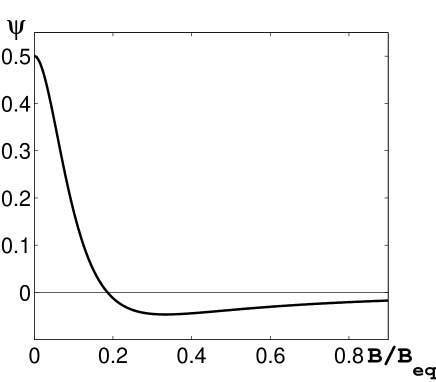
Figure 1: The function $\Psi(B/B_{\rm eq})$ for $q=5/3$.

In inhomogeneous turbulence there are also turbulent diamagnetic and paramagnetic effects. In particular, an inhomogeneity of the velocity fluctuations leads to a transport of mean magnetic flux from regions with high intensity of the velocity fluctuations (turbulent diamagnetism, see, e.g., Z57 ; KR80 ). On the other hand, an inhomogeneity of magnetic fluctuations due to the small-scale dynamo causes turbulent paramagnetic velocity, i.e., the magnetic flux is pushed into regions with high intensity of the magnetic fluctuations (see, e.g., VK83 ; RKR03 ). In order to determine the nonlinear turbulent diamagnetic and paramagnetic drift velocities ${\bf V}^{\rm eff}({\bf B})$ of the mean magnetic field, we use an identity: $V^{\rm(eff)}_{k}=\varepsilon_{kji}a_{ij}/2$, where the tensor $a_{ij}$ is determined by Eq. (LABEL:C1) in Appendix A. The inhomogeneities of the velocity and magnetic fluctuations of the background turbulence are characterized by the following parameters $\Lambda_{i}^{(v)}=\nabla_{i}\langle{\bf u}^{2}\rangle^{(0)}/\langle{\bf u}^{2}\rangle^{(0)}$ and $\Lambda_{i}^{(b)}=\nabla_{i}\langle{\bf b}^{2}\rangle^{(0)}/\langle{\bf b}^{2}\rangle^{(0)}$. The nonlinear effective drift velocity of the mean magnetic field is given by

$${\bf V}^{\rm eff}=-2\eta_{{}_{T}}[{\bf\Lambda}^{(v)}-\epsilon{\bf\Lambda}^{(m)}]\Psi_{1}(\beta)\;,$$ (14)

where the function $\Psi_{1}(\beta)$ and its asymptotic formulas are given in Appendix B. When $B\gg B_{\rm eq}/\sqrt{\rm Rm}$, Eqs. (11) and (14) yield

$${\bf V}^{\rm eff} = -2\eta_{{}_{T}}\biggl{[}{\bf\Lambda}^{(v)}-{\bf\Lambda}^{(m)}+{{\rm div}\,{\bf F}^{A}\over 4\eta_{{}_{T}}B^{2}\Psi(\beta)}\,{\bf\Lambda}^{(m)}\biggr{]}\Psi_{1}(\beta)\;.$$

The first term $\propto{\bf\Lambda}^{(v)}$ in Eq. (LABEL:RN43) determines the turbulent diamagnetic drift velocity while the second term $\propto{\bf\Lambda}^{(m)}$ describes the turbulent paramagnetic drift velocity. The last term $\propto{\rm div}\,{\bf F}^{A}$ in Eq. (LABEL:RN43) determines the turbulent diamagnetic drift velocity caused by magnetic fluctuations for $B<0.18\,B_{\rm eq}$. More general equation for ${\bf V}^{\rm eff}$ for anisotropic background turbulence is given by Eq. (43) in Appendix A.

IV Conclusions

In the present study we investigate nonlinear quenching of the turbulent magnetic diffusion and the effective drift velocity of the magnetic field in a developed two-dimensional MHD turbulence at large magnetic Reynolds numbers. We elucidate an important role of transport of the mean-square magnetic potential which strongly changes quenching properties of turbulent magnetic diffusion. In particular, we show that the catastrophic quenching of turbulent magnetic diffusion does not arises for the magnetic fields $B\gg B_{\rm eq}/\sqrt{\rm Rm}$ for a non-zero divergence of the flux of the mean-square magnetic potential. In this case the quenching of turbulent magnetic diffusion is independent of magnetic Reynolds number. This is similar to a three-dimensional MHD turbulence at large magnetic Reynolds numbers whereby the catastrophic quenching of the $\alpha$ effect does not occur when a divergence of the flux of the small-scale magnetic helicity is not zero. Note that in a two-dimensional MHD turbulence, the magnetic field may only decay, while in three-dimensional MHD turbulence magnetic field may grow by dynamo mechanism.

Note that a quenching of turbulent magnetic diffusivity in a ’wavy’ magnetohydrodynamic turbulence in two dimensions was recently studied in SD07 . They found that the turbulent magnetic diffusivity in the fourth-order does not vanish when the magnetic Reynolds number tends to infinity. In particularly, the second-order (quasi-linear) contribution to the spatial flux of the mean magnetic potential is quenched as ${\rm Rm}^{-1}$, while the fourth-order contribution to the flux is independent of ${\rm Rm}$. This implies that the turbulent magnetic diffusivity is not quenched catastrophically in the presence of dispersive waves which can transfer the mean-square magnetic potential. These findings are in an agrement with our results.

Appendix A Derivations of the nonlinear turbulent transport coefficients

We use equations for fluctuations of velocity and magnetic field written in a Fourier space and derive equations for the second moments in two-dimensional MHD turbulence using a procedure which is similar to that used in RK04 for a study of a three-dimensional MHD turbulence. In order to exclude the pressure term from the equation of motion (3) we determine $\mbox{\boldmath$\nabla$}{\bf\times}(\mbox{\boldmath$\nabla$}{\bf\times}{\bf u}).$ We also apply the two-scale approach, e.g., we use large-scale ${\bf R}$, ${\bf K}$ and small-scale ${\bf r}$, ${\bf k}$ variables (see, e.g., RS75 ). We assume that there exists a separation of scales, i.e., the maximum scale of turbulent motions $l_{0}$ is much smaller then the characteristic scale $L_{B}$ of inhomogeneities of the mean magnetic field. We derive equations for the following correlation functions: $f_{ij}({\bf k,R})=\hat{L}(u_{i};u_{j})$, $\;h_{ij}({\bf k,R})=\hat{L}(b_{i};b_{j})$ and $g_{ij}({\bf k,R})=\hat{L}(b_{i};u_{j})$, where

$$\hat{L}(a;c)=\int\langle a({\bf k}+{\bf K}/2)c(-{\bf k}+{\bf K}/2)\rangle$$

$$\times\exp{(i{\bf K}{\bf\cdot}{\bf R})}\,d{\bf K}\;.$$

The equations for these correlation functions are given by

$${\partial f_{ij}({\bf k})\over\partial t} = i({\bf k}{\bf\cdot}{\bf B})\Phi_{ij}^{(M)}+I^{f}_{ij}+F_{ij}+\hat{\cal N}f_{ij}\;,$$ (16)

$${\partial h_{ij}({\bf k})\over\partial t} = -i({\bf k}{\bf\cdot}{\bf B})\Phi_{ij}^{(M)}+I^{h}_{ij}+\hat{\cal N}h_{ij}\;,$$ (17)

$${\partial g_{ij}({\bf k})\over\partial t} = i({\bf k}{\bf\cdot}{\bf B})[f_{ij}({\bf k})-h_{ij}({\bf k})]+I^{g}_{ij}+\hat{\cal N}g_{ij}\;,$$

where hereafter we omit arguments $t$ and ${\bf R}$ in the correlation functions and neglect terms $\sim O(\nabla^{2}).$ Here $\Phi_{ij}^{(M)}({\bf k})=g_{ij}({\bf k})-g_{ji}(-{\bf k}),$ $\,F_{ij}({\bf k})=\langle\tilde{F}_{i}({\bf k})u_{j}(-{\bf k})\rangle+\langle u_{i}({\bf k})\tilde{F}_{j}(-{\bf k})\rangle,$ and ${\bf\tilde{F}}({\bf k})={\bf k}{\bf\times}({\bf k}{\bf\times}{\bf F}({\bf k}))/k^{2}\rho.$ The stirring force ${\bf F}({\bf k})$ is an external parameter, that determines the background turbulence. The source terms $I_{ij}^{f}$ , $\,I_{ij}^{h}$ and $I_{ij}^{g}$ which contain the large-scale spatial derivatives of the mean magnetic field and turbulence are given by

$$I_{ij}^{f} = {1\over 2}({\bf B}{\bf\cdot}\mbox{\boldmath$\nabla$})\Phi_{ij}^{(P)}+[g_{qj}({\bf k})(2P_{in}^{(2)}(k)-\delta_{in}^{(2)})$$

$$+g_{qi}(-{\bf k})(2P_{jn}^{(2)}(k)-\delta_{jn}^{(2)})]B_{n,q}-B_{n,q}k_{n}\Phi_{ijq}^{(P)}\;,$$

$$I_{ij}^{h} = {1\over 2}({\bf B}{\bf\cdot}\mbox{\boldmath$\nabla$})\Phi_{ij}^{(P)}-[g_{iq}({\bf k})\delta_{jn}^{(2)}+g_{jq}(-{\bf k})\delta_{in}^{(2)}]B_{n,q}$$ (20)

$$-B_{n,q}k_{n}\Phi_{ijq}^{(P)}\;,$$

$$I_{ij}^{g} = {1\over 2}({\bf B}{\bf\cdot}\mbox{\boldmath$\nabla$})(f_{ij}+h_{ij})+h_{iq}(2P_{jn}^{(2)}(k)-\delta_{jn}^{(2)})B_{n,q}$$ (21)

$$-f_{nj}B_{i,n}-B_{n,q}k_{n}(f_{ijq}+h_{ijq})\;,$$

where $P_{ij}^{(2)}(k)=\delta_{ij}^{(2)}-k_{ij}$, $\,k_{ij}=k_{i}k_{j}/k^{2}$, $\,\Phi_{ij}^{(P)}({\bf k})=g_{ij}({\bf k})+g_{ji}(-{\bf k}),$ and $B_{i,j}=\nabla_{j}B_{i},$ the terms $\hat{\cal N}f_{ij}$, $\,\hat{\cal N}h_{ij}$ and $\,\hat{\cal N}g_{ij}$ are the third-order moment terms appearing due to the nonlinear terms, $f_{ijq}=(1/2)\partial f_{ij}/\partial k_{q}$, and similarly for $h_{ijq}$ and $\Phi_{ijq}^{(P)}$. For the derivation of Eqs. (16)-(LABEL:B8) we use identities given in RK04 . We take into account that in Eq. (LABEL:B8) the terms with symmetric tensors with respect to the indexes ”i” and ”j” do not contribute to the mean electromotive force because ${\cal E}_{m}=\varepsilon_{mji}\,g_{ij}$.

We use the spectral $\tau$ approximation which postulates that the deviations of the third-moment terms, $\hat{\cal N}M^{(III)}({\bf k})$, from the contributions to these terms afforded by the background turbulence, $\hat{\cal N}M^{(III,0)}({\bf k})$, are expressed through the similar deviations of the second moments, $M^{(II)}({\bf k})-M^{(II,0)}({\bf k})$ [see Eq. (5)]. The superscript ${(0)}$ corresponds to the background turbulence. First, we solve Eqs. (16)-(LABEL:B8) neglecting the sources $I^{f}_{ij},I^{h}_{ij},I^{g}_{ij}$ with the large-scale spatial derivatives. Then we will take into account the terms with the large-scale spatial derivatives by perturbations. We assume that $\eta k^{2}\ll\tau^{-1}(k)$ and $\nu k^{2}\ll\tau^{-1}(k)$ for the inertial range of turbulent flow, where $\nu$ is the kinematic viscosity and $\eta$ is the magnetic diffusion due to the electrical conductivity of fluid. We also assume that the characteristic time of variation of the mean magnetic field ${\bf B}$ is substantially larger than the correlation time $\tau(k)$ for all turbulence scales. We split all correlation functions into symmetric and antisymmetric parts with respect to the wave number ${\bf k}$, e.g., $f_{ij}=f_{ij}^{(s)}+f_{ij}^{(a)},$ where $f_{ij}^{(s)}=[f_{ij}({\bf k})+f_{ij}(-{\bf k})]/2$ is the symmetric part and $f_{ij}^{(a)}=[f_{ij}({\bf k})-f_{ij}(-{\bf k})]/2$ is the antisymmetric part, and similarly for other tensors. Thus, in a steady-state Eqs. (16)-(LABEL:B8) yield:

$$\hat{f}_{ij}^{(s)}({\bf k}) \approx {1\over 1+2\psi}[(1+\psi)f_{ij}^{(0)}({\bf k})+\psi h_{ij}^{(0)}({\bf k})]\;,$$

$$\hat{h}_{ij}^{(s)}({\bf k}) \approx {1\over 1+2\psi}[\psi f_{ij}^{(0)}({\bf k})+(1+\psi)h_{ij}^{(0)}({\bf k})]\;,$$

$$\hat{g}_{ij}^{(a)}({\bf k}) \approx {i\tau({\bf k}{\bf\cdot}{\bf B})\over 1+2\psi}[f_{ij}^{(0)}({\bf k})-h_{ij}^{(0)}({\bf k})]\;,$$ (24)

where $\psi({\bf k})=2(\tau\,{\bf k}{\bf\cdot}{\bf B})^{2}$, $\,\hat{f}_{ij},\hat{h}_{ij}$ and $\hat{g}_{ij}$ are solutions without the sources $I^{f}_{ij},I^{h}_{ij}$ and $\,I^{g}_{ij}$. The correlation functions $\hat{f}_{ij}^{(a)}({\bf k})$, $\hat{h}_{ij}^{(a)}({\bf k})$ and $\hat{g}_{ij}^{(s)}({\bf k})$ vanish if we neglect the large-scale spatial derivatives, i.e., they are proportional to the first-order spatial derivatives.

Next, we take into account the large-scale spatial derivatives in Eqs. (16)-(LABEL:B8) by perturbations. Their effect determines the following steady-state equations for the second moments $\tilde{f}_{ij}$, $\tilde{h}_{ij}$ and $\tilde{g}_{ij}$:

$$\tilde{f}_{ij}^{(a)}({\bf k}) = i\tau({\bf k}{\bf\cdot}{\bf B})\tilde{\Phi}_{ij}^{(M,s)}({\bf k})+\tau I^{f}_{ij}\;,$$ (25)

$$\tilde{h}_{ij}^{(a)}({\bf k}) = -i\tau({\bf k}{\bf\cdot}{\bf B})\tilde{\Phi}_{ij}^{(M,s)}({\bf k})+\tau I^{h}_{ij}\;,$$ (26)

$$\tilde{g}_{ij}^{(s)}({\bf k}) = i\tau({\bf k}{\bf\cdot}{\bf B})(\tilde{f}_{ij}^{(a)}({\bf k})-\tilde{h}_{ij}^{(a)}({\bf k}))+\tau I^{g}_{ij}\;,$$

where $\tilde{\Phi}_{ij}^{(M,s)}=[\tilde{\Phi}_{ij}^{(M)}({\bf k})+\tilde{\Phi}_{ij}^{(M)}(-{\bf k})]/2.$ The solution of Eqs. (25)-(LABEL:B30) yield

$$\tilde{\Phi}_{ij}^{(M,s)}({\bf k}) = {\tau\over 1+2\psi}\{I^{g}_{ij}-I^{g}_{ji}+i\tau({\bf k}{\bf\cdot}{\bf B})(I^{f}_{ij}-I^{f}_{ji}$$ (28)

$$+I^{h}_{ji}-I^{h}_{ij})\}\;.$$

Substituting Eq. (28) into Eqs. (25)-(LABEL:B30) we obtain the final expressions in ${\bf k}$-space for the tensors $\tilde{f}_{ij}^{(a)}({\bf k})$, $\tilde{h}_{ij}^{(a)}({\bf k})$, $\tilde{g}_{ij}^{(s)}({\bf k})$ and $\tilde{\Phi}_{ij}^{(M,s)}({\bf k})$. In particular,

$$\tilde{\Phi}_{mn}^{(M,s)}({\bf k})={\tau(k)W(k)\langle{\bf u}^{2}\rangle^{(0)}\over(1+2\psi)^{2}}\biggl{[}(1+\epsilon)(1+2\psi)(\delta_{nj}^{(2)}\delta_{mk}^{(2)}$$

$$-\delta_{mj}^{(2)}\delta_{nk}^{(2)}+k_{nk}\delta_{mj}^{(2)}-k_{mk}\delta_{nj}^{(2)})-2(\epsilon+2\psi)(k_{nj}\delta_{mk}^{(2)}$$

$$-k_{mj}\delta_{nk}^{(2)})\biggr{]}\,B_{j,k}\;.$$ (29)

The correlation functions $\tilde{f}_{ij}^{(s)}({\bf k})$, $\tilde{h}_{ij}^{(s)}({\bf k})$ and $\tilde{g}_{ij}^{(a)}({\bf k})$ are of the order of $\sim O(\nabla^{2})$, i.e., they are proportional to the second-order spatial derivatives. Thus $\hat{g}_{ij}+\tilde{g}_{ij}$ is the correlation function of the cross-helicity, and similarly for other second moments. Now we calculate the mean electromotive force ${\cal E}_{i}({\bf r}=0)=(1/2)\varepsilon_{inm}\int\tilde{\Phi}_{mn}^{(M,s)}({\bf k})\,d{\bf k}$. Thus,

$${\cal E}_{i} = \varepsilon_{inm}\int{\tau\over 1+2\psi}\,[I^{g}_{mn}+i\tau({\bf k}{\bf\cdot}{\bf B})(I^{f}_{mn}-I^{h}_{mn})]\,d{\bf k}\;.$$

We use the following model of the background anisotropic and inhomogeneous two-dimensional MHD turbulence:

$$\langle u_{i}\,u_{j}\rangle^{(0)}({\bf k})=\langle{\bf u}^{2}\rangle^{(0)}\,W^{v}(k)\,\biggl{\{}(1-\sigma^{v})\Big{[}\delta_{ij}^{(2)}-k_{ij}$$

$$\quad\;+{i\over 2k^{2}}(k_{i}\Lambda_{j}^{(v)}-k_{j}\Lambda_{i}^{(v)})\Big{]}+\sigma^{v}\beta_{ij}\delta({\bf k}\cdot{\bf B})\biggr{\}}\;,$$ (31)

$$\langle b_{i}\,b_{j}\rangle^{(0)}({\bf k})=\langle{\bf b}^{2}\rangle^{(0)}\,W^{m}(k)\,\biggl{\{}(1-\sigma^{m})\Big{[}\delta_{ij}^{(2)}-k_{ij}$$

$$\quad\;+{i\over 2k^{2}}(k_{i}\Lambda_{j}^{(m)}-k_{j}\Lambda_{i}^{(m)})\Big{]}+\sigma^{m}\beta_{ij}\delta({\bf k}\cdot{\bf B})\biggr{\}}\;,$$

(32)

where $\delta_{ij}^{(2)}=\delta_{ij}-e_{i}e_{j}$, $\,\delta_{ij}$ is the Kronecker tensor, $e_{i}$ is the unit vector which is perpendicular to the plane of the two-dimensional MHD turbulence, $k_{ij}=k_{i}k_{j}/k^{2}$, $\,\sigma^{v}$ and $\sigma^{m}$ are the degrees of anisotropy of the velocity and magnetic fluctuations of the background turbulence, and $\sigma^{v}>\sigma^{m}$, $\,\beta_{ij}=B_{i}B_{j}/B^{2},$ $\,W^{v}(k)=W^{m}(k)=E(k)/2\pi k$. The energy spectrum of the velocity and magnetic fluctuations is $E(k)=k_{0}^{-1}\,(q-1)\,(k/k_{0})^{-q}$, the turbulent correlation time is $\,\tau(k)=2\tau_{0}(k/k_{0})^{1-q},$ where $1<q<3$ is the exponent of the energy spectrum, $k_{0}=1/l_{0},$ and $l_{0}$ is the maximum scale of turbulent motions, $\tau_{0}=l_{0}/u_{0}$, $\,u_{0}$ is the characteristic turbulent velocity in the scale $l_{0}$. The inhomogeneities of the velocity and magnetic fluctuations of the background turbulence are characterized by $\,\Lambda_{i}^{(v)}=\nabla_{i}\langle{\bf u}^{2}\rangle^{(0)}/\langle{\bf u}^{2}\rangle^{(0)}$ and $\Lambda_{i}^{(b)}=\nabla_{i}\langle{\bf b}^{2}\rangle^{(0)}/\langle{\bf b}^{2}\rangle^{(0)}$. Note that $\langle u_{i}\,b_{j}\rangle^{(0)}({\bf k})=0$. In Eqs. (31) and (32) we neglected small quadratic terms in the parameters $\Lambda_{i}^{(v)}$ and $\Lambda_{i}^{(b)}$.

After the integration in ${\bf k}$-space we obtain ${\cal E}_{i}=a_{ij}B_{j}+b_{ijk}B_{j,k},$ where $B_{j,k}=\nabla_{k}B_{j}$ and

$$a_{ij} = 2\eta_{{}_{T}}[(1-\sigma^{v})\Lambda_{n}^{(v)}-\epsilon(1-\sigma^{m})\Lambda_{n}^{(m)}]\,\varepsilon_{ipn}K_{pj}^{(1)}\;,$$

$$b_{ijk} = 2\eta_{{}_{T}}\biggl{[}[1-\sigma^{v}+\epsilon(1-\sigma^{m})]\,(\varepsilon_{ijk}K_{pp}^{(1)}-\varepsilon_{ijp}K_{pk}^{(1)})$$ (34)

$$-2\epsilon(1-\sigma^{m})\varepsilon_{ink}K_{nj}^{(1)}+2\,\varepsilon_{ink}\tilde{K}_{nj}^{(1)}[1-\sigma^{v}$$

$$-\epsilon(1-\sigma^{m})]\biggr{]}+2\eta_{{}_{T}}\beta_{pk}\,[(\sigma^{v}+\epsilon\sigma^{m})\varepsilon_{ijp}$$

$$-2\epsilon\sigma^{m}\,\varepsilon_{inp}({\bf e}{\bf\times}\mbox{\boldmath$\hat{\beta}$})_{n}({\bf e}{\bf\times}\mbox{\boldmath$\hat{\beta}$})_{j}]\;.$$

Here $\mbox{\boldmath$\hat{\beta}$}={\bf B}/B$,

$$K_{ij}^{(1)} = {1\over\pi}\int_{{\rm Rm}^{-c}}^{1}x\,K_{ij}[y(x)]\,dx\;,$$

$$\tilde{K}_{ij}^{(1)} = {1\over\pi}\int_{{\rm Rm}^{-c}}^{1}\;x\,y(x){dK_{ij}(y)\over dy}\,dx\;,$$

$$K_{ij}(y) = \int_{0}^{2\pi}{k_{ij}\over 1+y\cos^{2}\varphi}\,d\varphi=D_{1}(y)\delta_{ij}^{(2)}+D_{2}(y)\beta_{ij},$$

$$D_{1}(y) = {2\pi\over y}(\sqrt{y+1}-1),\;D_{2}(y)={2\pi\over y}\biggl{[}2-{y+2\over\sqrt{y+1}}\biggr{]},$$

$$y(x) = {2\beta^{2}\over x^{\gamma}}\;,\quad\gamma={2\,(2-q)\over q-1}\;,\quad c={q-1\over 3-q}\;,$$

$\beta=4\,(B/B_{\rm eq})$ and $B_{\rm eq}=\sqrt{\langle{\bf u}^{2}\rangle^{(0)}}$ is the equipartition field. For $q=5/3$ the parameters $\gamma=1$ and $c=1/2$, and for $q=3/2$ the parameters $\gamma=2$ and $c=1/3$.

To determine the nonlinear turbulent magnetic diffusion ${\eta}_{ij}({\bf B})$ we use an identity: $\eta_{ij}=(\varepsilon_{ikp}b_{jkp}+\varepsilon_{jkp}b_{ikp})/4$. The nonlinear turbulent magnetic diffusion coefficient along the mean magnetic field, $\eta_{{}_{B}}$, and the cross-field turbulent magnetic diffusion coefficient, $\eta_{{}_{\perp}}$, are given by:

$$\eta_{{}_{B}} = 2\eta_{{}_{T}}\biggl{[}\sigma^{v}-\epsilon\sigma^{m}+[1-\sigma^{v}-\epsilon(1-\sigma^{m})]\Psi_{1}(\beta)\biggr{]}\;,$$

$$\eta_{{}_{\perp}} = 2\eta_{{}_{T}}[1-\sigma^{v}-\epsilon(1-\sigma^{m})]\Psi(\beta)\;,$$ (36)

where $\eta_{{}_{T}}=l_{0}\,u_{0}/2$, the functions $\Psi(\beta)$, $\,\Psi_{1}(\beta)$ and their asymptotic formulas are given in Appendix B, $\beta=4\,(B/B_{\rm eq})$, $\,B_{\rm eq}=\sqrt{\langle{\bf u}^{2}\rangle^{(0)}}$ is the equipartition field and the parameter $\epsilon=\langle{\bf b}^{2}\rangle^{(0)}/\langle{\bf u}^{2}\rangle^{(0)}$. To derive Eqs. (LABEL:B36) and (36) we used the following identities:

$$e_{i}\varepsilon_{ijp}\beta_{pk}\nabla_{k}B_{j}=\Delta_{x}A\;,\quad e_{i}\varepsilon_{ipk}\beta_{pj}\nabla_{k}B_{j}=\Delta_{y}A\;,$$

$$e_{i}\varepsilon_{inp}\beta_{pk}\nabla_{k}B_{j}({\bf e}{\bf\times}\mbox{\boldmath$\hat{\beta}$})_{n}({\bf e}{\bf\times}\mbox{\boldmath$\hat{\beta}$})_{j}=\Delta_{x}A\;,$$

where ${\bf B}={\bf e}_{x}B$. The nonlinear turbulent magnetic diffusion coefficients $\eta_{{}_{B}}$ and $\eta_{{}_{\perp}}$ for $\sigma^{v}=\sigma^{m}=0$ are given in Sec. III [see Eqs. (6) and (7)].

Now we determine the parameter $\epsilon=\langle{\bf b}^{2}\rangle^{(0)}/\langle{\bf u}^{2}\rangle^{(0)}$ using budget equation for the evolution of the mean-square magnetic potential $\langle a^{2}\rangle$ [see Eq. (8)]. To this end we determine the energy of magnetic fluctuations $\langle{\bf b}^{2}\rangle$ which is obtained from Eq. (LABEL:B24) by the integration in ${\bf k}$-space. The result is given by

$$\langle{\bf b}^{2}\rangle = {\langle{\bf u}^{2}\rangle^{(0)}\over 2}\Big{[}(1-\sigma^{v})[1-\phi(\beta)]+\epsilon[1+\sigma^{m}$$ (37)

$$+\phi(\beta)(1-\sigma^{m})]\Big{]}\;,$$

where the function $\phi(\beta)$ and its asymptotic formulas are given in Appendix B. Combining Eq. (37) with the steady-state solution of Eq. (8) we determine the parameter $S(\epsilon)\equiv 1-\sigma^{v}-\epsilon(1-\sigma^{m})$:

$$S(\epsilon) = 2\biggl{[}{1-\sigma^{v}\over 1-\sigma^{m}}+{\rm Rm}\,{{\rm div}\,{\bf F}^{A}\over 4\eta_{{}_{T}}\,B_{\rm eq}^{2}}\biggr{]}\,\biggl{[}{1+\sigma^{m}\over 1-\sigma^{m}}+\phi(\beta)$$ (38)

$$+2\,{\rm Rm}\,\Psi(\beta)\,{B^{2}\over B_{\rm eq}^{2}}\biggr{]}^{-1}\;.$$

When $B\gg B_{\rm eq}/\sqrt{\rm Rm}$, Eq. (38) yields the parameters $\epsilon$:

$$\epsilon = {1\over 1-\sigma^{m}}\biggl{[}1-\sigma^{v}-{{\rm div}\,{\bf F}^{A}\over 4\eta_{{}_{T}}B^{2}\Psi(\beta)}\biggr{]}\;.$$ (39)

Using Eqs. (LABEL:B36), (36) and (39) we obtain the nonlinear turbulent magnetic diffusion in two directions:

$$\eta_{{}_{B}} = {2\eta_{{}_{T}}\over 1-\sigma^{m}}\,\biggl{[}\sigma^{v}-\sigma^{m}+{{\rm div}\,{\bf F}^{A}\over 4\eta_{{}_{T}}B^{2}\Psi(\beta)}[\sigma^{m}$$ (40)

$$+(1-\sigma^{m})\,\Psi_{1}(\beta)]\biggr{]}\;,$$

$$\eta_{{}_{\perp}} = {{\rm div}\,{\bf F}^{A}\over 2B^{2}}\;.$$ (41)

Note that there is a small range of the magnitudes of the mean magnetic field when there can be an anomalous behaviour of the nonlinear turbulent magnetic diffusion. At $B\to 0.18\,B_{\rm eq}$ the function $\Psi(\beta)$ changes sign (see Fig. 1). On the other hand, the function $S(\epsilon)$ changes sign for slightly larger value of the magnetic field $B>0.18\,B_{\rm eq}$ [see Eq. (38)]. Therefore, this implies that at $B>0.18\,B_{\rm eq}$ the nonlinear turbulent magnetic diffusion can be anomalously large. The width of the range of the anomalous behaviour of the nonlinear turbulent magnetic diffusion is very small, $\delta B\sim 1/{\rm Rm}$. In this range the steady-state solution of Eq. (8) for $B>0.18\,B_{\rm eq}$ does not exist.

To determine the nonlinear effective drift velocity ${\bf V}^{\rm eff}({\bf B})$ of the mean magnetic field we use an identity: $V^{\rm(eff)}_{k}=\varepsilon_{kji}a_{ij}/2$, which yields

$${\bf V}^{\rm eff}=-2\eta_{{}_{T}}[(1-\sigma^{v}){\bf\Lambda}^{(v)}-\epsilon(1-\sigma^{m}){\bf\Lambda}^{(m)}]\Psi_{1}(\beta)\;,$$

(42)

where the function $\Psi_{1}(\beta)$ and its asymptotic formulas are given in Appendix B. When $B\gg B_{\rm eq}/\sqrt{\rm Rm}$, Eqs. (39) and (42) yield

$${\bf V}^{\rm eff} = -2\eta_{{}_{T}}\biggl{[}(1-\sigma^{v})\,({\bf\Lambda}^{(v)}-{\bf\Lambda}^{(m)})$$ (43)

$$+{{\rm div}\,{\bf F}^{A}\over 4\eta_{{}_{T}}B^{2}\Psi(\beta)}\,{\bf\Lambda}^{(m)}\biggr{]}\Psi_{1}(\beta)\;.$$

The nonlinear effective drift velocity ${\bf V}^{\rm eff}({\bf B})$ of the mean magnetic field for $\sigma^{v}=\sigma^{m}=0$ is given in Sec. III [see Eq. (LABEL:RN43)].

Appendix B Functions $\Psi(\beta)$, $\,\Psi_{1}(\beta)$ and $\phi(\beta)$

In this section we present the functions $\Psi(\beta)$, $\,\Psi_{1}(\beta)$ and $\phi(\beta)$ used in Sec. III:

$$\Psi(\beta) = {1\over\pi}\int_{{\rm Rm}^{-c}}^{1}\;x\biggl{[}1+2y(x){d\over dy}\biggr{]}\,[D_{1}(y)+D_{2}(y)]\,dx,$$

$$\Psi_{1}(\beta) = {1\over\pi}\int_{{\rm Rm}^{-c}}^{1}\;x\biggl{[}1+2y(x){d\over dy}\biggr{]}D_{1}(y)\,dx\;,$$

$$\phi(\beta) = {1\over 2\pi}\int_{{\rm Rm}^{-c}}^{1}\;[2D_{1}(y)+D_{2}(y)]\,dx\;.$$

These functions for $q=5/3$ are given by

$$\Psi(\beta) = {\beta^{4}\over 6}\,[M(\beta)-M(\beta\,{\rm Rm}^{1/4})]+{25\over 2}L(\beta,{\rm Rm})\;,$$

$$\Psi_{1}(\beta) = {1\over 6\beta^{2}}\{2-[2-5\beta^{2}(1-3\beta^{2})]\,\sqrt{2\beta^{2}+1}\}$$ (45)

$$+{5\over 2}L(\beta,{\rm Rm})\;,$$

$$\phi(\beta) = {1\over 2}\,\biggl{[}\sqrt{2\beta^{2}+1}-{2\over\beta^{2}}\,L(\beta,{\rm Rm})\biggr{]}\;,$$ (46)

$$L(\beta,{\rm Rm}) = \beta^{4}\biggl{[}\ln{\sqrt{2\beta^{2}\sqrt{\rm Rm}+1}-1\over\sqrt{2\beta^{2}\sqrt{\rm Rm}+1}+1}$$ (47)

$$-\ln{\sqrt{2\beta^{2}+1}-1\over\sqrt{2\beta^{2}+1}+1}\biggr{]}\;,$$

$$M(y) = {1\over y^{4}\sqrt{2y^{2}+1}}\,\biggl{[}5[1-5y^{2}(1+6y^{2})]$$ (48)

$$+{2\over y^{2}}(1-\sqrt{2y^{2}+1})\biggr{]}\;.$$

Asymptotic formulas for the functions $\Psi(\beta)$, $\,\Psi_{1}(\beta)$ and $\phi(\beta)$ are as follows. For $\beta\ll{\rm Rm}^{-1/4}$ these functions are given by

$$\Psi(\beta) = {1\over 2}\,\biggl{[}1-9\beta^{2}+{25\over 2}\beta^{4}\ln{\rm Rm}\biggr{]}\;,$$

$$\Psi_{1}(\beta) = {1\over 2}\,\biggl{[}1-3\beta^{2}+{5\over 2}\beta^{4}\ln{\rm Rm}\biggr{]}\;,$$

$$\phi(\beta) = 1-{1\over 2}\beta^{2}\ln{\rm Rm}\;,$$

for ${\rm Rm}^{-1/4}\ll\beta\ll 1$ they are given by

$$\Psi(\beta) = {1\over 2}\,\biggl{[}1-9\beta^{2}+50\beta^{4}|\ln\beta|\biggr{]}\;,$$

$$\Psi_{1}(\beta) = {1\over 2}\,\biggl{[}1-3\beta^{2}+10\beta^{4}|\ln\beta|\biggr{]}\;,$$

$$\phi(\beta) = 1-2\beta^{2}\,|\ln\beta|\;,$$

and for $\beta\gg 1$ these functions are given by

$$\Psi(\beta) = -{1\over 3\beta^{2}}\,\biggl{[}1-{1.7\over\beta}\biggr{]}\;,$$

$$\Psi_{1}(\beta) = {1\over 3\beta^{2}}\;,\quad\phi(\beta)=-{0.24\over\beta}\;.$$

References

- (1) H. K. Moffatt, Magnetic Field Generation in Electrically Conducting Fluids (Cambridge University Press, New York, 1978).
- (2) E. Parker, Cosmical Magnetic Fields (Oxford University Press, New York, 1979).
- (3) F. Krause and K. H. Rädler, Mean-Field Magnetohydrodynamics and Dynamo Theory (Pergamon, Oxford, 1980).
- (4) Ya. B. Zeldovich, A. A. Ruzmaikin and D. D. Sokoloff, Magnetic Fields in Astrophysics (Gordon and Breach, New York, 1983).
- (5) A. Ruzmaikin, A. M. Shukurov and D. D. Sokoloff, Magnetic Fields of Galaxies (Kluwer Academic, Dordrecht, 1988).
- (6) M. Stix, The Sun: An Introduction (Springer, Berlin and Heidelberg, 1989).
- (7) R. Kulsrud, Ann. Rev. Astron. Astrophys. 37, 37 (1999), and references therein.
- (8) M. Ossendrijver, Astron. Astrophys. Rev. 11, 287 (2003), and references therein.
- (9) A. Brandenburg and K. Subramanian, Phys. Rept. 417, 1 (2005), and references therein.
- (10) F. Cattaneo and S. I. Vainshtein, Astrophys. J. 376, L21 (1991).
- (11) S. I. Vainshtein and F. Cattaneo, Astrophys. J. 393, 165 (1992).
- (12) A. Gruzinov and P. H. Diamond, Phys. Rev. Lett., 72, 1651 (1994); Phys. Plasmas 2, 1941 (1995); Phys. Plasmas 3, 1853 (1996).
- (13) F. Cattaneo and D. W. Hughes, Phys. Rev. E 54 R4532 (1996).
- (14) P. H. Diamond, D. W. Hughes and Eun-jin Kim, In. Fluid Dynamics and Dynamos in Astrophysics and Geophysics, reviews, the Durham Symposium on Astrophysical Fluid Mechanics, 29 July - 8 August 2002. Eds. by A. M. Soward, C. A. Jones, D. W. Hughes and N. O. Weiss (CRC Press, Boca Raton, 2005), p. 145.
- (15) P. H. Diamond, S.-I. Itoh, K. Itoh and T. S. Hahm, Plasma Phys. Control. Fusion 47, R35 (2005).
- (16) Ya. B. Zeldovich, Zh. Eksp. Teor. Fiz. 31, 154 (1956) [Sov. Phys. JETP 4, 460 (1957)].
- (17) T. S. Iroshnikov, Astron. Zh. 40, 742 (1963) [Sov. Astron. 7, 566 (1964)].
- (18) R. H. Kraichnan, Phys. Fluids 8, 1385 (1965).
- (19) E. G. Blackman and G. B. Field, Astrophys. J. 534, 984 (2000).
- (20) N. Kleeorin, D. Moss, I. Rogachevskii and D. Sokoloff, Astron. Astrophys. 361, L5 (2000); 387, 453 (2002); 400, 9 (2003).
- (21) N. Kleeorin, K. Kuzanyan, D. Moss, I. Rogachevskii and D. Sokoloff, Astron. Astrophys. 409, 1097 (2003).
- (22) I. Rogachevskii, N. Kleeorin and E. Liverts, Geophys. Astrophys. Fluid Dynam. 100, 537 (2006).
- (23) I. Rogachevskii and N. Kleeorin, Phys. Rev. E 70, 046310 (2004); 75, 046305 (2007).
- (24) A. S. Monin and A. M. Yaglom, Statistical Fluid Mechanics (MIT Press, Cambridge, Massachusetts, 1975), Vol. 2.
- (25) W. D. McComb, The Physics of Fluid Turbulence (Clarendon, Oxford, 1990).
- (26) S. A. Orszag, J. Fluid Mech. 41, 363 (1970).
- (27) A. Pouquet, U. Frisch, and J. Leorat, J. Fluid Mech. 77, 321 (1976).
- (28) N. Kleeorin, I. Rogachevskii, and A. Ruzmaikin, Zh. Eksp. Teor. Fiz. 97, 1555 (1990) [Sov. Phys. JETP 70, 878 (1990)].
- (29) N. Kleeorin, M. Mond, and I. Rogachevskii, Astron. Astrophys. 307, 293 (1996).
- (30) E. G. Blackman and G. Field, Phys. Rev. Lett. 89, 265007 (2002); Phys. Fluids 15, L73 (2003).
- (31) G. Field and E. G. Blackman, Astrophys. J. 572, 685 (2002).
- (32) A. Brandenburg, P. Käpylä, and A. Mohammed, Phys. Fluids 16, 1020 (2004).
- (33) A. Brandenburg and K. Subramanian, Astron. Astrophys. 439, 835 (2005).
- (34) S. Sur, K. Subramanian and A. Brandenburg, Mon. Not. Roy. Astron. Soc. 376, 1238 (2007).
- (35) S. I. Vainshtein and L. L. Kitchatinov, Geophys. Astrophys. Fluid Dynam. 24, 273 (1983).
- (36) K.-H. Rädler, N. Kleeorin and I. Rogachevskii, Geophys. Astrophys. Fluid Dyn. 97, 249 (2003).
- (37) S. R. Keating and P. H. Diamond, J. Fluid Mech., submitted (2007).
- (38) P. H. Roberts and A. M. Soward, Astron. Nachr. 296, 49 (1975).