Abstract

We discuss the lightest scalar resonances, $f_{0}(600)$, $\kappa(800)$, $a_{0}(980)$ and $f_{0}(980)$ in the extended Nambu Jona-Lasinio model. We find that the model parameters can be tuned, but unnaturally, to accommodate those scalars except the $f_{0}(980)$. We also discuss problems encountered in the K Matrix unitarization approximation by using $N_{c}$ counting technique.

Key words: Nambu Jona-Lasinio model; Scalars
PACS: 12.39.Fe, 14.40.-n

1 Introduction

The original model of Nambu and Jona-Lasinio [2] (NJL)was proposed as a dynamical model of the strong interactions between nucleons and pions, before the invention of QCD. In this model pions appear as the massless composite bosons associated with the dynamical spontaneous breakdown of the chiral symmetry of the initial lagrangian. Even after the invention of QCD, the NJL model or the extended NJL (ENJL) model still serves as a useful tool widely discussed in the literature when discussing low energy strong interaction physics at the quark-level, starting from last seventies and eighties [3, 4]. More recent extensive reviews can be found in [5].

The ENJL model provides a natural extension and hence is considered more general than the linear sigma model or the model in which the $\rho$ meson takes the role of a massive gauge boson of the isospin symmetry. The ENJL model attempts to provide a unified description to both the scalar sector as well as the vector sector, in a chiral symmetric way. However, there have been controversies for a long time on the spectrum of the lowest lying scalar nonet in strong interactions. This situation is also reflected in the early studies on ENJL models. In Ref. [6], the ENJL model is used to study the lightest scalar nonet, and it is found that, $m_{a}=500$MeV, $m_{K_{*}}=840$MeV, $m_{\sigma_{0}}\simeq 760$MeV, $m_{\sigma_{8}}=950$MeV. The mass of $a_{0}(980)$ meson (which is degenerate to the SU(2) $\sigma$ in Ref. [6]) could not be explained by the NJL model itself, and the mass difference is ascribed to a possible $qq\bar{q}\bar{q}$ content in the physical $a_{0}$. In Ref. [7] the role of QCD $U_{A}(1)$ anomaly is considered and a sum rule is obtained between the mass of scalars and the pseudoscalars in the NJL model via ’t Hooft’s instanton interaction [8]. The instanton effect will break the degeneracy between the octet and the singlet, which lifts the former and suppresses the latter. Starting with a ‘bare’ quarkonium mass of 1100MeV in Ref. [7], $U_{A}(1)$ splits the $0^{+}$ nonet into a singlet $\thicksim 1000$MeV and an octet $\thicksim 1300$MeV. Broken $SU_{f}(3)$ further splits the masses so that one gets: $m_{a_{0}}=1320$MeV, $m_{\sigma_{8}}=1590$MeV, $m_{\sigma_{0}}=1000$MeV, $m_{K^{*}_{0}}=1430$MeV. Apparently this assignment is not for the lightest scalars since it contains a heavy $a_{0}$. The above work did not include $\kappa$ (or $K^{*}_{0}(800)$) in their lightest scalar nonet. This situation is improved by Volkov $et$ $al$ [9] who discussed the NJL model with the ’t Hooft interaction (which splits the mass between $a_{0}$ and $\sigma$) and find $m_{a_{0}}=810$MeV, $m_{\sigma}=550$MeV, $m_{\sigma^{\prime}}=1130$MeV, $m_{K_{0}^{*}}=960$MeV. Nevertheless there is an apparent problem with these results, that is for a small $\sigma$ mass around 550MeV (and also a small mass for the $\kappa$), it does not possess enough phase space to develop a large width for the $\sigma$ as is revealed by recent determinations. More recent work [10, 11] observed that there is growing evidence that $a_{0}(980)$, $K_{0}^{*}(800)$ or $\kappa$, as well as $f_{0}(600)$ or $\sigma$ and $f_{0}(980)$, are members of the low-lying scalar nonet. Nevertheless Ref. [10] suffers from the similar problem as in Ref. [9], it also gives a rather small mass of $\sigma$ with which it is difficult to explain the large width of the sigma simultaneously.

On the other side, progress has been made in recent few years, demonstrating the existence of the light and broad $\sigma$ (or $f_{0}(600)$) and $\kappa$ resonances [12]. The pole locations of $\sigma$ and $\kappa$ are determined using dispersive approaches [13]–[17]. This new information on the pole locations urges and enables us to watch more carefully the dynamics with respect to the lightest scalars, within the scheme of the extended NJL model, which is the purpose of this paper.

The basic idea of the present paper is outlined already in Ref. [18], where we pointed out that in order to understand correctly the mass relations among lightest scalars one has to take into account the additional information provided by the widths of these scalars, ranging from a few tens MeV to a few hundred MeV. Especially when there appears a large width, since it is an unambiguous signal for strong interactions in the given channel, the bare mass spectrum at tree level has to be strongly distorted. A certain unitarization procedure is necessary to explore the relation between the pole mass parameters and the bare mass parameters put in the lagrangian. For example it is suggested in Ref. [18] that a $\sigma$ pole locates at $\sqrt{z}=m-i\Gamma/2=470-285i$ MeV corresponds to a bare mass $M_{\sigma}\simeq 930MeV$ with some uncertainties.

This paper is devoted to the study on the lightest scalar resonances within the ENJL model. Our aim is to explore whether one can explain within the model, at least at qualitative level, the masses and widths of $\sigma(600)$, $K_{0}^{*}(800)$, $a_{0}(980)$ and $f_{0}(980)$ simultaneously. We find that the model encounters serious difficulties for its own reason, though it can be finely tuned, unnaturally, to explain the masses and widths of $f_{0}(600)$, $K_{0}^{*}(800)$ and $a_{0}(980)$. However in such a case the ENJL model can no longer explain the vector meson spectrum. Furthermore, if we only focus on the scalar sector and ignore the problem with vector meson mass spectrum, there still remains a problem that the $f_{0}(980)$ is not possible to be described as a member of the scalar octet: it has a too small mass.

This paper is organized as following: section 1 is the introduction, in section 2, we make a short review on the ENJL model, especially those materials being used in this paper. In section 3, we reconstruct the mass relations of scalar mesons and also discuss the tree-level decay widths of scalars. In section 4, using $K$ matrix method we construct a unitarized scattering amplitude and find pole locations in each channel, numerical results are listed and discussed. We also discuss the $N_{c}$ dependence of pole trajectories. Our discussion is also slightly generalized by including the unitarization approximation of the more general resonance chiral theory. In section 5, we draw our conclusions on the nature of light scalars, based on our study on the $K$ matrix unitarization of the ENJL model amplitude.

2 The ENJL model

This section reviews how to derive an effective meson chiral lagrangian, involving both scalars and vector mesons, from a four fermi interaction. Combining with ’t Hooft’s interaction lagrangian the ENJL model provides the basic tool for our study. The method introduced in this section is standard [3, 4, 5].

2.1 Bosonization of the ENJL model

We start from the four quark interactions

$${\cal L}_{\rm QCD} \rightarrow \sum_{i}\bar{q}(i\partial\hbox to0.0pt{\hss$/$}-{\cal M})q+{\cal L}_{\rm NJL}^{\rm S,P}+{\cal L}_{\rm NJL}^{\rm V,A}+{\cal O}\left(1/\Lambda_{\chi}^{4}\right),$$ (1)

$${\rm with}\hskip 42.67912pt{\cal L}_{\rm NJL}^{\rm S,P} = \frac{\displaystyle 8\pi^{2}G_{S}}{\displaystyle N_{c}\Lambda_{\chi}^{2}}\,{\displaystyle\sum_{i,j}}\left(\overline{q}^{i}_{R}q^{j}_{L}\right)\left(\overline{q}^{j}_{L}q^{i}_{R}\right)$$

$${\rm and}\hskip 42.67912pt{\cal L}_{\rm NJL}^{\rm V,A} = -\frac{\displaystyle 8\pi^{2}G_{V}}{\displaystyle N_{c}\Lambda_{\chi}^{2}}\,{\displaystyle\sum_{i,j}}\left[\left(\overline{q}^{i}_{L}\gamma^{\mu}q^{j}_{L}\right)\left(\overline{q}^{j}_{L}\gamma_{\mu}q^{i}_{L}\right)+\left(L\rightarrow R\right)\right]\ ,$$

where $i,j$ are flavor indices, $\Psi_{R,L}\equiv(1/2)\left(1\pm\gamma_{5}\right)\Psi$ and the couplings $G_{S}$ and $G_{V}$ are dimensionless quantities. We adopt the same symbols and definitions as in the third reference of Ref. [5]. We introduce three complex $3\times 3$ auxiliary field matrices $M(x)$, $L_{\mu}(x)$ and $R_{\mu}(x)$, which under the chiral group $G=SU_{L}(3)\times SU_{R}(3)$ transform as

$$M \to g_{R}Mg_{L}^{\dagger},$$

$$L_{\mu}\to g_{L}L_{\mu}g_{L}^{\dagger}\,\,\, \,\,\,R_{\mu}\to g_{R}R_{\mu}g_{R}^{\dagger}.$$ and (2)

By polar decomposition

$$M=U\tilde{H}=\xi H\xi,$$ (3)

with $U$ unitary, $\tilde{H}$ (and $H$) hermitian and

$$\xi(\Phi)\to g_{R}\xi(\Phi)h^{\dagger}(\Phi,g_{L,R})=h(\Phi,g_{L,R})\xi(\Phi)g_{L}^{\dagger},$$ (4)

where $\xi(\Phi)\xi(\Phi)=U$. From the transformation laws of $M$ and $\xi$, it follows that $H$ transforms homogeneously, i.e.,

$$H\to h(\Phi,g_{L,R})Hh^{\dagger}(\Phi,g_{L,R}).$$ (5)

We can reconstruct the vector fields

$$W_{\mu}^{\pm}=\xi L_{\mu}\xi^{\dagger}\pm\xi^{\dagger}R_{\mu}\xi.$$ (6)

The transformation properties is

$$W_{\mu}^{\pm}\to h(\Phi,g)W_{\mu}^{\pm}h^{\dagger}(\Phi,g)\ .$$ (7)

After some deduction, one obtains in the Euclidean space the effective action $\Gamma_{eff}(M_{Q},\xi,\sigma,W_{\mu}^{\pm};v,a,s,p)$ in terms of the new auxiliary field variables and in the presence of the external field sources $v_{\mu}$, $a_{\mu}$, $s$ and $p$ [5],

$$e^{\Gamma_{eff}(M_{Q},\xi,\sigma,W_{\mu}^{\pm};v,a,s,p)}=$$

$$\hbox{exp}\left(-\int d^{4}x\left\{{N_{c}\Lambda_{\chi}^{2}\over 8\pi^{2}G_{S}(\Lambda_{\chi})}trH^{2}+{N_{c}\Lambda_{\chi}^{2}\over 16\pi^{2}G_{V}(\Lambda_{\chi})}{1\over 4}tr(W_{\mu}^{+}W_{\mu}^{+}+W_{\mu}^{-}W_{\mu}^{-})\right\}\right)\times$$

$$\int{\cal D}\bar{Q}{\cal D}Q\hbox{exp}\int d^{4}x\bar{Q}{\cal D}_{E}Q,$$ (8)

where ${\cal D}_{E}$ denotes the Euclidean Dirac operator

$${\cal D}_{E}=\gamma_{\mu}\nabla_{\mu}-{1\over 2}(\Sigma-\gamma_{5}\Delta)-H(x)$$ (9)

with $\nabla_{\mu}$, the covariant derivative

$$\nabla_{\mu}=\partial_{\mu}+\Gamma_{\mu}-{i\over 2}\gamma_{5}(\xi_{\mu}-W_{\mu}^{(-)})-{i\over 2}W_{\mu}^{(+)}$$ (10)

and

$$\Sigma=\xi^{\dagger}\cal{M}\xi^{\dagger}+\xi\cal{M}^{\dagger}\xi$$ (11)

$$\Delta=\xi^{\dagger}\cal{M}\xi^{\dagger}-\xi\cal{M}^{\dagger}\xi\ .$$ (12)

The quantities $\Gamma_{\mu}$ and $\xi_{\mu}$ are those

$$\Gamma_{\mu}={1\over 2}\{\xi^{\dagger}[\partial_{\mu}-i(v_{\mu}+a_{\mu})]\xi+\xi[\partial_{\mu}-i(v_{\mu}-a_{\mu})]\xi^{\dagger}\}\ ,$$ (13)

and

$$\xi_{\mu}=i\{\xi^{\dagger}[\partial_{\mu}-i(v_{\mu}+a_{\mu})]\xi-\xi[\partial_{\mu}-i(v_{\mu}-a_{\mu})]\xi^{\dagger}\}=i\xi^{\dagger}D_{\mu}U\xi^{\dagger}=\xi_{\mu}^{\dagger}\ .$$ (14)

The effective action is in the basis of constituent chiral quark fields $Q$,

$$Q_{L}=\xi q_{L}\,,\,\bar{Q}_{L}=\bar{q}_{L}\xi^{\dagger}\,;\,Q_{R}=\xi^{\dagger}q_{R}\,,\,\bar{Q}_{R}=\bar{q}_{R}\xi\ .$$ (15)

With

$$\hbox{exp }\int{\cal D}\bar{Q}{\cal D}Q\hbox{exp}\int d^{4}x\bar{Q}{\cal D}_{E}Q=\hbox{det}{\cal D}_{E},$$ (16)

we can get the effective action

$$\Gamma_{eff}(M_{Q},\xi,\sigma,W_{\mu}^{\pm};v,a,s,p)$$

$$=-\int d^{4}x\left\{{N_{c}\Lambda_{\chi}^{2}\over 8\pi^{2}G_{S}}trH^{2}+{N_{c}\Lambda_{\chi}^{2}\over 16\pi^{2}G_{V}}{1\over 4}tr(W_{\mu}^{+}W_{\mu}^{+}+W_{\mu}^{-}W_{\mu}^{-})\right\}$$

$$+\ln(\hbox{det}|{\cal D}_{E}|).$$ (17)

Using proper time regularization and heat-kernel expansion method [19], we get an effective Lagrangian of meson fields from the ENJL model. One can also use other regularization method [20] to get similar effective lagrangian.

2.2 Gap Equation and the ’t Hooft Interaction

Here, we are looking for translational invariant solutions which minimize the effective action, i.e.,

$${\delta\Gamma_{eff}(H,...)\over\delta H}|_{L_{\mu}=R_{\mu}=0,\xi=1,H=<H>;v_{\mu}=a_{\mu}=s=p=0}=0,$$ (18)

where $<H>=\hbox{diag}(M_{u},M_{d},M_{s})$. The minimum is reached when all the eigenvalues of $<H>$ are equal, i.e.,

$$<H>=M_{Q}1$$ (19)

and the minimum condition leads to the so called gap equation

$$\int d^{4}x\,\mathrm{Tr}(x|D_{E}^{-1}|x)|_{L_{\mu}=R_{\mu}=0,\xi=1,H=M_{Q};v_{\mu}=a_{\mu}=s=p=0}=-4M_{Q}{N_{c}\Lambda_{\chi}^{2}\over 16\pi^{2}G_{S}(\Lambda_{\chi})}\int d^{4}x,$$ (20)

where $M_{Q}$ is the constituent quark mass. From Eq. (20) one further gets,

$$M_{Q}={G_{S}\over\Lambda_{\chi}^{2}}\Gamma(-1,\frac{M_{Q}^{2}}{\Lambda_{\chi}^{2}})M_{Q}^{3},$$ (21)

where $\Gamma(-1,x)$ denotes the incomplete gamma function

$$\Gamma(n-2,x=\frac{M_{Q}^{2}}{\Lambda_{\chi}^{2}})=\int_{M_{Q}^{2}/\Lambda_{\chi}^{2}}^{\infty}{dz\over z}e^{-z}z^{n-2};\,\,\,\,\,n=1,2,3,...\ .$$ (22)

The Eq. (21) is obtained using proper time regularization method used in this paper. The gap equation (21) is obtained without introducing the current quark masses. We can introduce the current quark mass through the external source field $s=\hbox{diag}(m_{u},m_{d},m_{s})$, $m_{u,d,s}$ is the current quark mass. Unlike the method used in Ref. [11] we just use the gap equation without explicit $SU_{f}(3)$ breaking to avoid the complicated calculation in heat-kernel expansion. We need to shift the the SU(3) singlet field $\sigma_{0}$ and the octet filed $\sigma_{8}$ again in the broken phase to get the physical fields with zero vacuum expectation values in the effective lagrangian.

The next step is to add the ’t Hooft interaction [8], $\beta(\hbox{det}H+\hbox{det}H^{\dagger})$, where $\beta$ is a constant characterizing the strength of the anomaly contribution. We get the modified gap equation,

$$\displaystyle{{\delta\Gamma_{eff}^{\prime}(H,...)\over\delta H}|_{H=<H>}} ={\delta\Gamma_{eff}(H,...)\over\delta H}|_{H=<H>}+\beta{\delta(\hbox{det}H+\hbox{det}H^{\dagger})\over\delta H}$$ (23)

$$\Rightarrow \frac{\Lambda_{\chi}^{2}}{G_{S}}-\Gamma(-1,x)M_{Q}^{2}=\frac{8\pi^{2}\beta M_{Q}}{N_{C}}.$$

2.3 The Effective Lagrangian and its couplings

In the ENJL model, we have six input parameters:

$$G_{S},\,\ G_{V},\,\ \Lambda_{x},\,\ m_{q},\,\ m_{s},\,\ \hbox{and}\ \,\ \beta\ .$$ (24)

The gap equation

$$\frac{\Lambda_{\chi}^{2}}{G_{S}}-\Gamma(-1,x)M_{Q}^{2}=\frac{8\pi^{2}\beta M_{Q}}{N_{C}}$$ (25)

introduces a constituent chiral quark mass parameter $M_{Q}$, and the ratio

$$x=\frac{M_{Q}^{2}}{\Lambda_{x}^{2}}.$$ (26)

We can replace the parameters $G_{S}$, $G_{V}$ and $\Lambda_{x}$ with $x$, $M_{Q}$, and

$$g_{A}={1\over 1+4G_{V}x\Gamma(0,x)}\ ,$$ (27)

characterizing the $\pi$ – $A_{1}$ mixing. In the limit of $G_{V}\to 0~{}(g_{A}\to 1)$, the ENJL model goes back to the NJL model.

The effective Lagrangian can be written down in the form:

$${\cal L}_{eff} = \frac{1}{4}f_{\pi}^{2}\,\left[\,\mbox{tr}\,\left(D_{\mu}UD^{\mu}U^{\dagger}\right)+\,\mbox{tr}\,\left(\chi U^{\dagger}+U^{\dagger}\chi\right)\right]$$ (28)

$$-\frac{1}{4}\,\mbox{tr}\,\,[V_{\mu\nu}V^{\mu\nu}-2M_{V}^{2}V_{\mu}V^{\mu}]$$

$$-\frac{1}{4}\,\mbox{tr}\,\,[A_{\mu\nu}A^{\mu\nu}-2M_{A}^{2}A_{\mu}A^{\mu}]$$

$$-\frac{1}{2\sqrt{2}}\left[f_{V}\,\mbox{tr}\,\left(V_{\mu\nu}f_{+}^{\mu\nu}\right)+ig_{V}\,\mbox{tr}\,\left(V_{\mu\nu}[\xi^{\mu},\xi^{\nu}]\right)+f_{A}\,\mbox{tr}\,\left(A_{\mu\nu}f_{-}^{\mu\nu}\right)\right]$$

$$+\cal{L}_{S}$$

$$+\tilde{L}_{1}\left(\,\mbox{tr}\,\,D_{\mu}U^{\dagger}D^{\mu}U\right)^{2}+\tilde{L}_{2}\,\mbox{tr}\,\left(D_{\mu}U^{\dagger}D_{\nu}U\,\mbox{tr}\,\,D^{\mu}U^{\dagger}D^{\nu}U\right)$$

$$+\tilde{L}_{3}\,\mbox{tr}\,\left(D_{\mu}U^{\dagger}D^{\mu}UD_{\nu}U^{\dagger}D^{\nu}U\right)$$

$$+\tilde{L}_{5}\,\mbox{tr}\,\left[D_{\mu}U^{\dagger}D^{\mu}U\left(\chi^{\dagger}U+U^{\dagger}\chi\right)\right]+\tilde{L}_{7}\left[\,\mbox{tr}\,(U\chi^{{\dagger}}-\chi U^{{\dagger}})\right]^{2}$$

$$+\tilde{L}_{8}\,\mbox{tr}\,\left(\chi^{\dagger}U\chi^{\dagger}U+\chi U^{\dagger}\chi U^{\dagger}\right)+\tilde{H}_{2}\,\mbox{tr}\,\left(\chi^{\dagger}\chi\right)\,,$$

where

$$\mathcal{L}_{S} = {1\over 2}\,\mbox{tr}\,\left(d_{\mu}Sd^{\mu}S-M_{S}^{2}S^{2}\right)+c_{m}\,\mbox{tr}\,\left(S\chi^{+}\right)+c_{d}\,\mbox{tr}\,\left(S\xi_{\mu}\xi^{\mu}\right)+...$$ (29)

The relevant coupling constants in above lagrangians are listed in the Appendix A. We do not integrate out the heavy resonances (vectors, axial-vectors and scalars) to get the low energy constants $L_{i}$, therefore we use $\tilde{L}_{i}$ to distinguish them from the LECs in chiral perturbation theory [21].

Attempts have been made in expressing the low energy constants in terms of QCD operators [22]. Nevertheless most reliable estimates and determinations at this stage are from phenomenological studies [23]. The couplings $f_{V}$ and $g_{V}$ can be then determined from the decay $\rho^{0}\to e^{+}e^{-}$ and $\rho\to\pi\pi$ respectively, with the result

$$|f_{V}|=0.20\,\,\,{\hbox{and}}\,\,\,|g_{V}|=0.090.$$

The decay $a_{1}\to\pi\gamma$ fixes the coupling

$$|f_{A}|=0.097\pm 0.022.$$

For the scalar couplings $c_{m}$ and $c_{d}$, there exists controversy due to the lowest scalar multiplet. One can take the scalar multiplet including $a_{0}(980)$ as the lightest scalar nonet as in Ref. [23]. Using the $a_{0}\to\eta\pi$ decay width and assuming the scalar saturation of $L_{5}$ and $L_{8}$ to determine $c_{m}$ and $c_{d}$, in this way one computes with $M_{S}=M_{a_{0}}=983$ MeV,

$$|c_{d}| = 32\,\hbox{MeV},$$

$$|c_{m}| = 42\,\hbox{MeV},$$

$$\hbox{and}\,\,\,c_{d}c_{m} > 0.$$ (30)

Alternately, the authors of Ref. [24] consider the scalar multiple to be around $1.2\sim 1.4$ GeV as the lightest scalars in the $L_{S}$ and gives the value $c_{d}=c_{m}\sim f_{\pi}/2$.

The coupling constants, $c_{m}$, $c_{d}$, $f_{V}$, $f_{A}$ and $G_{V}$ have been given from the ENJL model in Ref. [25]. As will be shown later, the most important parameter appearing in this paper is the axial vector coupling $g_{A}$. The preferred value of $g_{A}$ is found to be around 0.6 in Ref. [25]. In Ref. [26], an estimation gives $g_{A}=\frac{1}{2}$ under some additional theoretical constraints.

3 Scalar Mass Spectrum and Decays of Scalar Mesons

3.1 Scalar Mass Spectrum

The scalar nonet is denoted as the following,

$$S(x)=\left(\begin{array}[]{ccc}{\frac{a^{0}}{\sqrt{2}}}+{\frac{\sigma_{0}}{\sqrt{3}}+}\frac{\sigma_{8}}{\sqrt{6}}&a^{+}&\kappa^{+}\\ a^{-}&-{\frac{a^{0}}{\sqrt{2}}+}\frac{\sigma_{0}}{\sqrt{3}}+{\frac{\sigma_{8}}{\sqrt{6}}}&\kappa^{0}\\ \kappa^{-}&\overline{\kappa}^{0}&\frac{\sigma_{0}}{\sqrt{3}}-\sqrt{\frac{2}{3}}\sigma_{8}\end{array}\right)\ .$$ (31)

Mass relations for the scalar nonet can be extracted from the effective lagrangian. Firstly for the charge and flavor neutral scalars there is a mixing term:

$${\cal L}_{mixing}=M_{00}^{2}\sigma_{0}^{2}+M_{08}^{2}\sigma_{0}\sigma_{8}+M_{88}^{2}\sigma_{8}^{2}\ .$$ (32)

One finds

$$M_{00}^{2}=\frac{1}{3}(2M_{\kappa}^{2}+M_{a_{0}}^{2})-g_{A}M_{th}^{2},$$

$$M_{88}^{2}=\frac{1}{3}(4M_{\kappa}^{2}-M_{a_{0}}^{2}),$$

$$M_{08}^{2}=-\frac{4\sqrt{2}}{3}(M_{\kappa}^{2}-M_{a_{0}}^{2}),$$ (33)

where

$$M_{th}^{2}=m_{\eta}^{2}+m_{\eta^{\prime}}^{2}-2m_{K}^{2}=4\beta M_{Q}^{3}(\frac{1}{2f_{K}^{2}-f_{\pi}^{2}}+\frac{2}{f_{\pi}^{2}})\ ,$$ (34)

and

$$M_{a_{0}}^{2}\simeq 3g_{A}m_{\pi}^{2}+4M_{Q}^{2}+\frac{2}{3}g_{A}M_{th}^{2},$$

$$M_{\kappa}^{2}\simeq 3g_{A}m_{K}^{2}+4M_{Q}^{2}+\frac{2}{3}g_{A}M_{th}^{2},$$ (35)

and $M_{Q}$ is the constituent quark mass. The Eq. (3.1) is only exact in the leading order of cutoff dependence. After diagonalizing Eq. (32) one gets the masses for mass eigenstates and the mixing angle,

$$M^{2}_{\sigma}=\frac{1}{2}\left[2M_{\kappa}^{2}-g_{A}M_{th}^{2}-\sqrt{(M_{00}^{2}-M_{88}^{2})^{2}+(M_{08}^{2})^{2}}\right],$$

$$M^{2}_{\sigma^{\prime}}=\frac{1}{2}\left[2M_{\kappa}^{2}-g_{A}M_{th}^{2}+\sqrt{(M_{00}^{2}-M_{88}^{2})^{2}+(M_{08}^{2})^{2}}\right],$$

$$\tan 2\theta={\frac{4\sqrt{2}}{3}(M_{\kappa}^{2}-M_{a_{0}}^{2})\over\frac{2}{3}(M_{\kappa}^{2}-M_{a_{0}}^{2})+g_{A}M_{th}^{2}}\ .$$ (36)

From (35) and (36), one gets immediately two sum rules:

$$2M^{2}_{\kappa}-M^{2}_{\sigma}-M^{2}_{\sigma^{\prime}}\simeq g_{A}M^{2}_{th},$$ (37)

$$M^{2}_{\kappa}-M^{2}_{a}\simeq 3g_{A}(m^{2}_{K}-m^{2}_{\pi}).$$ (38)

The first sum rule Eq. (37) has been obtained in Ref. [7]. The second sum rule Eq. (38) is in qualitative agreement with the results given in Ref. [10]. They are the consequence of $U_{A}(1)$ breaking in the ENJL model combined with linear $SU(3)$ symmetry breaking terms. If we do not include the anomaly contribution in the scalar mass spectrum, just setting $M_{th}^{2}=0$ in (35), we can find the mixing angle $\theta=(\arctan 2\sqrt{2})/2=\theta_{id}\simeq 35.26^{\circ}$. Then the $\sigma$ is a pure non-strange state, and the $\sigma^{\prime}$ is purely strange. The scalar masses become

$$M_{a_{0}}^{2}=M^{2}_{\sigma}=3g_{A}m_{\pi}^{2}+4M_{Q}^{2}\ ,$$

$$M_{\kappa}^{2}=3g_{A}m_{K}^{2}+4M_{Q}^{2}\ ,$$

$$M^{2}_{\sigma^{\prime}}=2M^{2}_{\kappa}-m^{2}_{\pi}\ .$$ (39)

Before jumping into more detailed numerical calculations, we can make some simple estimates and discussions at qualitative level with Eqs. (37) and (38). The first important thing to notice is that, as already emphasized in Ref. [18], the scalar masses appeared in Eqs. (37) and (38) are only ‘bare’ mass parameters appeared in the lagrangian, which, when the interaction becomes strong, can be totally different from the pole mass positions. The large width of $\sigma$ (or $\kappa$) is an unambiguous signal for a strong $\sigma\pi\pi$ (or $\kappa K\pi$) interactions. The large widths are quite often ignored when discussing the mass spectrum in the literature. It is often attempted to set up SU(3) mass relations among pole mass parameters $m$. However, a light $\sigma$ with a mass around 500MeV as a bare parameter appeared in the lagrangian can hardly produce a large width, in any model calculations. On the other side, the parameter $M$ for $\sigma$ or $\kappa$ can be estimated to be $M_{\sigma}\simeq 930$MeV and $M_{\kappa}\simeq 1380$MeV with sizable error bars [18]. Qualitatively speaking the stronger the resonance couples to the $\pi\pi$ continuum, the larger the deviation is between $m$ and $M$. Instead of comparing different $m$, one should firstly examine the relations between different “bare” mass parameters, $M$. Since the former quantities associated with large widths are severely distorted by the strong couplings to the pseudo-goldstone pairs, it is not suitable to use them to discuss the SU(3) mass relations. For example, we have

$$m_{\sigma}<m_{\kappa}<m_{a_{0}}\ ,$$ (40)

but actually the mass relation should be read as

$$1GeV\simeq M_{\sigma}\lesssim M_{a_{0}}<M_{\kappa}\ .$$ (41)

The mass of $\sigma^{\prime}$ is unavoidably large, with or without anomaly contributions. If we include the contribution of the ’t Hooft interaction, taking for example $M_{\kappa}=1.2GeV$, $M_{\sigma}\simeq 1GeV$, $g_{A}=0.6$, and $M_{th}^{2}=0.72GeV^{2}$, we get $M_{a_{0}}=1.02GeV$, $M_{\sigma^{\prime}}=1.2GeV$, $\theta\simeq 23.59^{\circ}$, and

$${\sigma\choose\sigma^{\prime}}\simeq\left(\begin{array}[]{cc}0.98&-0.20\\ 0.20&0.98\end{array}\right){\sigma_{ns}\choose-\sigma_{s}}$$ (42)

from Eqs. (35)-(38). If $g_{A}$ grows larger, the mass of $\sigma^{\prime}$ will be heavier. If we neglect the contribution of ’t Hooft interaction, and taking for example $M_{a}=M_{\sigma}\simeq 1GeV$ and $g_{A}=0.6$, we get $M_{\kappa}\simeq 1.19GeV,M_{\sigma^{\prime}}\simeq 1.35GeV$. If $g_{A}$ grows larger, masses of $\kappa$ and $\sigma^{\prime}$ will be pushed higher too. In both cases, with and without ’t Hooft term’s contribution, the $\sigma^{\prime}$ is problematic within the present scenario to be identified with the physical $f_{0}(980)$ state, simply because the former is too heavy. As will be seen in the discussion given later in this paper, that in order to explain the large width of $\sigma$ and $\kappa$ in a dynamical approach, one needs large values of $M_{Q}$ and $g_{A}$. The immediate consequence is that the ENJL model would predict an unacceptably large vector meson spectrum and hence fails to give the correct description to the mass of $\rho$ and $a_{1}$ mesons. The reason for this is because in ENJL model the correlation between the parameters of scalar sector and the vector seems to be too strong. This is not necessary for hadron physics – in resonance chiral theory, for example, there is no such strong correlations between the two sectors. Hence we will in the following only focus upon the scalar sector and ignore the problem in the vector sector. The experience we are going to obtain is still meaningful – if not within the ENJL model itself – in a more general background, as in the resonance chiral theory.

In the scalar sector, as we mentioned above, the problem remains how to identify the $f_{0}(980)$ resonance. A possible way to solve the $\sigma^{\prime}$ and the $f_{0}(980)$ problem is that since the bare state $\sigma^{\prime}$ is much heavier it may mix with $f_{0}(1370)$, etc. Without instanton effects, the $\sigma$ and $\sigma^{\prime}$ are ideally mixed and the latter is $|\bar{s}s>$. When the instanton effects are taken into account, $\sigma^{\prime}$ may contain a sizable $|\bar{n}n>$ content and hence may have a sizable mixing with the heavier scalar like $f_{0}(1370)$, thus reducing to some extent its mass. On the other side, one may identify the $\sigma^{\prime}$ simply to the $f_{0}(1500)$ state, since the mass can be quite close to each other and the latter is known to be mainly $\bar{s}s$ state. Then the $f_{0}(980)$ may be considered as a $\bar{K}K$ molecule [28, 29]. Considering the complicated situation about $f_{0}(980)$, a convincing explanation to $f_{0}(980)$ is out of the range of the present discussion and remains to be explored in future.

There are six parameters ($M_{Q}$, $x$, $g_{A}$, $m_{q}$, $m_{s}$ and $\beta$) in the ENJL model under investigation, and there are different ways to choose physical parameters to be fit. For example, we can fit $f_{\pi}$, $f_{K}$, $m_{\pi}$, $m_{K}$, $M_{th}$ (through $M_{th}^{2}=m_{\eta}^{2}+m_{\eta^{\prime}}^{2}-2m_{K}^{2}$), $m_{\rho}$ and the bare mass of $\sigma$. In the old literature, the bare mass of $\sigma$ (and also $a_{0}$ in the absence of anomaly) is typically 500 – 600MeV which is too small. Since roughly there is a mass relation in the chiral limit, $M_{\sigma}\sim 2M_{Q}$ [30], it is difficult to increase the bare mass of $\sigma$ within the ENJL model. Adding ’t Hooft interaction term will even further decrease the singlet $\sigma$ mass. So the first thing to be noticed is that it is somewhat unnatural to assign a sigma mass of order 1GeV in the ENJL model. As can be seen from table 1, the $x$ parameter is quite large, which is not natural in the cutoff effective lagrangian approach. Another problem is that $f_{V}$ ($\simeq$ 0.1) can no longer be fitted well to its experimental value ($\simeq 0.2$). Also the current strange quark mass gets unnaturally large when $g_{A}$ increases. Furthermore, besides these problems, it is clear from table 1 that when $g_{A}$ gets larger the mass of $\sigma^{\prime}$ is enhanced and deviates more and more from the narrow width state $f_{0}(980)$. Barring this problem, setting $M_{\sigma}\sim 1$GeV, the bare mass of the $\kappa$ resonance is an output which turns out to be $\sim 1.3$GeV and agrees within expectation. Table 1 provides several fit values.

Table 1: Experimental values and predictions of the ENJL model for the various low energy parameters discussed in the text. All dimensional quantities are in MeV except $m_{th}^{2}$ in GeV.

	exp.	fit 1	fit 2	fit 3	fit 4	fit 5
	value
$f_{\pi}$	92.4	92.6	92.5	92.3	92.0	91.7
$f_{K}$	112.0	102.0	106.7	112.4	118.9	136.1
$m_{\pi}$	137.3	137.2	137.2	137.2	137.3	137.3
$m_{K}$	495.7	495.6	495.7	495.6	495.6	495.4
$m_{th}^{2}$	0.727	0.645	0.44	0.31	0.23	0.16
$M_{\sigma}^{\ddagger}$	$\thicksim 930$	856	869	881	892	903.8
$M_{a}$	984.7	1039	1025	1016	1010	1004
$M_{\kappa}^{\ddagger}$	$\thicksim 1400$	1227	1274	1330	1391	1458
$M_{\sigma^{\prime}}$	980	1360	1456	1560	1669	1784
$x$		0.175	0.234	0.295	0.356	0.419
$M_{Q}$		397.0	395.3	394.1	393.3	393.3
$g_{A}$		$0.5^{*}$	$0.6^{*}$	$0.7^{*}$	$0.8^{*}$	$0.9^{*}$
$m_{q}$		4.6	6.9	9.6	12.7	16.1
$m_{s}$		114.	172.4	240.0	317.1	403.5
$\beta$		9.2	6.7	5.2	4.0	3.1

(^‡) Corresponding to bare masses discussed in the text.
($*$) Values of $g_{A}$ are fixed in the fits.

3.2 Decays of Scalar Mesons

A serious investigation of the scalar mass spectrum unavoidably requires taking unitarization into account. But before doing that, in this section we will discuss at tree level the decay widths of light scalars, which can be helpful, though very rough, in the understanding of strong interaction dynamics behind. For example, if the decay width in a given channel in perturbation calculation is small then we can judge that the interaction is not strong and the difference between bare mass and pole mass is unimportant. If on the other hand the decay width is very large then one may claim that the difference between bare mass and pole mass ought to be large. In the latter case one has to find more reliable method to handle the strong interaction dynamics rather than calculating decay width perturbatively.

We use the effective lagrangian to calculate the decay rates of a scalar into two pseudoscalars, at tree level. The $\sigma$ decay width is expressed below,

$$\Gamma_{\sigma->\pi\pi}=3\Gamma_{\sigma->\pi_{0}\pi_{0}}$$

$$=\frac{g_{A}}{16\pi M_{\sigma}f_{\pi}^{2}}\sqrt{1-\frac{4m_{\pi}^{2}}{M_{\sigma}^{2}}}(g_{A}(M_{\sigma}^{2}-2m_{\pi}^{2})+m_{\pi}^{2})^{2}(\cos\theta+\frac{\sin\theta}{\sqrt{2}})^{2}\ ,$$ (43)

where $\theta$ is the scalar meson mixing angel defined by Eq. (36). When $\theta$ is equal to $\theta_{id}$, the decay width is maximal. From Fig. 1, one realizes that in order to explain the large discrepancy between $m_{\sigma}$ and $M_{\sigma}$, $g_{A}$ should not be small, for otherwise the decay width is small and the interaction will not be strong enough to develop a big difference between $m_{\sigma}$ and $M_{\sigma}$.

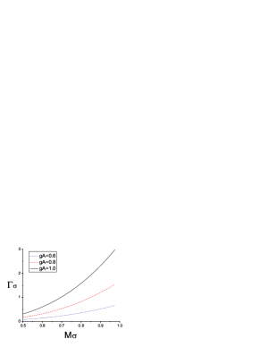
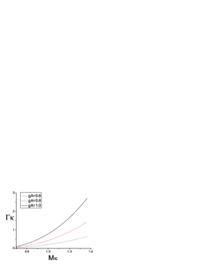
Figure 1: The decay widths of $\sigma$ (left) and $\kappa$ (right) as a function of scalar mass $M_{\sigma}$ and $M_{\kappa}$, respectively; for $g_{A}$=1.0, 0.8 and 0.6. The units are in GeV.

Especially, from the Fig. 1, we realize that the light $M_{\sigma}\thicksim 500MeV$ and $M_{\kappa}\thicksim 700MeV$ can not produce large widths. In the SU(3) limit, we have $g_{\sigma\pi\pi}=g_{\kappa K\pi}$ and the width is proportional to $g_{A}^{3}$. The only possibility in both cases to get a large width is to increase the bare mass parameters. We also plot the decay width of $a_{0}\rightarrow\pi\eta_{8}$ in Fig. 2. The decay width of $a_{0}$ is much smaller comparing with that of $\sigma$ and $\kappa$ simply because of SU(3) symmetry. See Fig. 2 for illustration. Therefore, as revealed by Figs. 1 and 2, the ENJL model does provide a possibility in its parameter space to explain the observed scalar spectrum and the vastly different widths simultaneously, at least qualitatively.

Figure 2: The decay width of $(a_{0}\rightarrow\pi\eta_{8})$ as a function of bare scalar mass $M_{a_{0}}$ for values of $g_{A}$=1.0, 0.8 and 0.6 respectively.

4 Pole masses of scalar resonances in the ENJL model

4.1 The K matrix unitarization and the pole positions

Certain unitarization approximation is necessary when a large width is involved. The unitarization method has been applied to (resonance) chiral perturbation theory amplitudes, and also to linear sigma models in the literature (see for example Ref. [32, 24]). To our knowledge, this paper is the first attempt to apply unitarization to ENJL amplitudes. The scattering amplitudes for two pseudoscalars to two pseudoscalars are easily obtainable at tree level in the ENJL model, The single channel K–matrix unitarization is the following:

$$T=\frac{T^{\mathrm{tree}}}{1-i\rho T^{\mathrm{tree}}}\ .$$ (44)

We use the $K$ Matrix amplitude determined from ENJL model to search for pole positions of scalars, which are not found in the previous literature. The results, corresponding to several choices of $g_{A}=0.6,0.7$ and 0.8, are listed in table 2. In the unitarized amplitudes there are actually quite a few poles in each channel, on both sheets. Nevertheless in each channel there is only one pole that falls on the real axis in the large $N_{c}$ limit which is just the input pole in the lagrangian. However, the results listed in table 2 should not be understood as accurate in any sense. On the contrary, it is known that the $K$ matrix results are crude for derivative coupling theories [33]. The results given in table 2 only provide a qualitative guide to the underlining dynamics: when $g_{A}$ is small the coupling strength between $\sigma$ and $\pi\pi$ is small and the width of $\sigma$ is also small. The mass of the $\sigma$ found from the unitarized amplitude is therefore very close to its input value. However, when $g_{A}$ increases up to, for example, 0.8, the width of $\sigma$ becomes large, and the pole mass $m_{\sigma}$ becomes totally different from the input bare mass, $M_{\sigma}$.

Table 2: Scalar pole masses

	fit 2 ($g_{A}=0.6$)	fit 3 ($g_{A}=0.7$)	fit 4 ($g_{A}=0.8$)
$\pi\pi\rightarrow\pi\pi$	$985\pm 133i$	$1161\pm 229i$	$544\pm 306i$
$\pi K\rightarrow\pi K$	$1423\pm 153i$	$1629\pm 202i$	$801\pm 360i$ ∗
$\pi\eta\rightarrow\pi\eta$	$1030\pm 31i$	$1016\pm 45i$	$1000\pm 60i$

^∗: The $N_{c}$ trajectory is marginal.

4.2 Pole trajectories with respect to the variation of $N_{c}$

As stated in last section that, all poles listed in table 2 fall on the real axis in the large $N_{c}$ limit. However, there are other poles on the second sheet and it is checked that they all go to $\infty$ on the complex $s$ plane when $N_{c}\to\infty$. Hence these states are dynamically generated. As discussed in section 4.1, for small values of $g_{A}$ (for example, fit 2 and fit 3) the $\sigma$ pole from the ENJL lagrangian has a rather small width and a large mass around 1GeV (as an input), but it is observed that in such a case there still exists a light and broad dynamical pole which disappears when $N_{c}\to\infty$. This pole, being dynamical, is certainly not the $\sigma$ pole responsible for chiral symmetry breaking in the ENJL model, since the latter is well monitored and falls on the real axis in the large $N_{c}$ limit. One may even further ask the question whether the experimentally observed $f_{0}(600)$ is the $\sigma$ responsible for chiral symmetry breaking (In the present situation corresponding to the light and broad resonance when $g_{A}$ is large as in fit 4), or a dynamically generated light and broad resonance, which is not the $\sigma$, when $g_{A}$ is small. To understand why there appears a ‘dynamical pole’ we recall that in general the tree level IJ=00 channel $\pi\pi$ elastic scattering amplitude, in the chiral limit, may be written as

$$T_{C.A.}=\frac{s}{16\pi f_{\pi}^{2}}\,,$$

$$T_{4}=\frac{s^{2}}{24\pi f_{\pi}^{4}}\triangle\,,\,\,(\triangle=22{\tilde{L}}_{1}+14{\tilde{L}}_{2}+11{\tilde{L}}_{3})$$

$$T_{S}=\frac{c_{d}^{2}}{16\pi f_{\pi}^{4}}(s-2M_{\sigma}^{2}+\frac{3s^{2}}{M_{\sigma}^{2}-s}+\frac{2M_{\sigma}^{4}}{s}\ln[1+\frac{s}{M_{\sigma}^{2}}]),\,\,\,$$ (45)

where $c_{d}\sim O(\sqrt{N_{c}})$ and $\tilde{L_{i}}$ are obtained by integrating out all resonance fields except scalars. The above expressions generally depict resonance chiral theory amplitudes including the ENJL model. The pole position in the chiral limit is determined by the equation

$$1+i(T_{CA}+T_{4}+T_{S})=0.$$ (46)

In Eq. (46) if we set $T_{4}$ and $T_{s}$ vanishing, we get the ‘current algebra sigma’ pole as already discussed in Ref. [33]. The $N_{c}$ dependence of the ‘current algebra sigma’ pole position is $\sqrt{s_{pole}}\sim\sqrt{N_{c}}$ and is ruled out through the study of Ref. [33, 34]. If setting $T_{4}=0$ and $\sqrt{2}c_{d}/f_{\pi}=1$ in Eq. (4.2) we recover the linear $\sigma$ model amplitude. In such a case the $\sigma$ resonance is light and broad when the bare mass of $\sigma$ is around 1GeV. In general, however, if we neglect the logarithm term in Eq. (46), which is suppressed when $s$ is large, it is not difficult to show that on the second sheet there exists, except the stable pole in the large $N_{c}$ limit, another pole with the property $s_{pole}\sim\sqrt{N_{c}}$ on the second sheet of complex s plane. Notice that dynamical pole obtained from Eq. (46) contains a different $N_{c}$ behavior comparing with the ‘current algebra $\sigma$’: the latter behaves as $\sqrt{s_{pole}}\sim\sqrt{N_{c}}$. The different $N_{c}$ dependence of the pole trajectory actually reminds us that the property of the so called ‘dynamical’ pole can be highly (unitarization) model dependent.

To prove the illegality of the light and broad dynamical pole generated from simple $K$ matrix unitarization of the tree level ENJL amplitude when $g_{A}$ is small, we make use of the low energy matching method developed in Ref. [35] (see also Ref. [34]). For $\pi\pi$ scattering $S$ matrix poles (on the second sheet) obey one relation:

$$\sum_{R}\frac{G_{R}}{M_{R}^{2}-4m_{\pi}^{2}}\sim O(N_{c}^{-1})\,,$$ (47)

where $M_{R}^{2}$ and $G_{R}$ are functions of the pole mass $z_{0}$ of resonance $R$ [15]:

$$M_{R}^{2}(z_{0})=\mathrm{Re}(z_{0})+\frac{\mathrm{Im}(z_{0})\mathrm{Im}[z_{0}\rho(z_{0})]}{\mathrm{Re}[z_{0}\rho(z_{0})]},$$ (48)

$$G_{R}(z_{0})=\frac{\mathrm{Im}(z_{0})}{\mathrm{Re}[z_{0}\rho(z_{0})]},\,\,$$ (49)

$$\rho(z_{0})=\sqrt{1-4m_{\pi}^{2}/z_{0}}\ .$$ (50)

No matter where on the second sheet does the pole locate, one always has ${G_{R}}/{(M_{R}^{2}-4m_{\pi}^{2})}>0$. The pole solution of Eq. (4.2) with the property $s_{pole}\sim\sqrt{N_{c}}$ corresponds to $M_{R}^{2}\propto\textit{O}(\sqrt{N_{c}})$ and $G_{R}\propto\textit{O}(1)$. Its contribution to the $l.h.s$ of Eq. (47) is $\textit{O}(1/\sqrt{N_{c}})$, meanwhile, the right-hand side is $\textit{O}(1/N_{c})$. The only possibility to satisfy Eq. (47) is that the contribution of a such ‘dynamical’ pole is canceled by a spurious pole on the physical sheet, whose contribution is also of order of $\textit{O}(1/\sqrt{N_{c}})$. This is just the case what we found from solutions of Eq. (4.2). Hence we demonstrate that the dynamical light and broad pole in the ENJL model, generated in the present simple $K$ matrix unitarization, is spurious.

We can also check the [1,1] Padé amplitude. The pole position of the [1,1] Padé amplitude is determined by the equation, in the chiral limit,

$$T_{2}-(T_{4}+T_{s}-i|T_{2}|^{2})=0$$

$$\sim\frac{s}{16\pi f_{\pi}^{2}}-\frac{s^{2}}{24\pi f_{\pi}^{4}}\Delta-\frac{c_{d}^{2}}{16\pi f_{\pi}^{4}}(s-2M_{\sigma}^{2}+\frac{3s^{2}}{M_{\sigma}^{2}-s})+i(\frac{s}{16\pi f_{\pi}^{2}})^{2}=0.$$ (51)

As before we neglect the logarithm term in above. It is straightforward to show that if no accidental cancelation occurs, when $N_{c}\to\infty$, there exist two poles on the second sheet of complex s plane, one is on the real axis and the other remains on the complex s plane: $s_{pole}\propto\textit{O}(1)$. At the same time, a spurious pole on the first sheet will be found, which is also $s_{pole}\propto\textit{O}(1)$. The latter exactly cancels the second sheet pole to meet the $N_{c}$ order of the $l.h.s$ of Eq. (47). Hence the dynamical pole with $s_{pole}\propto\textit{O}(1)$ found from the amplitude (4.2) is also a spurious one. Therefore the situation as described by Eq. (4.2) is quite different from the Padé amplitudes constructed from pure chiral perturbation theory [37, 38]. The latter is obtained by further integrating out the explicit scalar degree of freedom. There one does find that the dynamical pole falls on the real axis in the $N_{c}\to\infty$ limit.

5 Discussions and Conclusions

In this paper we discuss the possibility whether one can understand the light and broad $\sigma$ and $\kappa$, together with the narrow $a_{0}(980)$ and $f_{0}(980)$ in a same SU(3) nonet, in the ENJL model. We find that the ENJL model is quite reluctant for this picture. One difficulty is that the $\sigma^{\prime}$ resonance is simply too heavy to be identified as the $f_{0}(980)$ meson. One has to call for other mechanisms for the rescue. For example, the mixing with $f_{0}(1370)$ and/or $f_{0}(1500)$; or that $f_{0}(980)$ is simply a $\bar{K}K$ molecular state [29, 36]. Beside this difficulty, however, the ENJL model can give a rough but unified description to the light and broad $\sigma$, $\kappa$ and the narrow $a_{0}(980)$. For sufficiently large $g_{A}$ and an input bare $\sigma$ mass around 1GeV, a simple unitarization approximation generates a light and broad $\sigma$ resonance. The difference comes from the fact that the $\sigma$ couples very strongly to $\pi\pi$ continuum, hence its pole location is severely distorted. The price paid for this picture is that the $g_{A}$ and $M_{Q}$ parameter have to be unnaturally large. As a consequence, the ENJL model is no longer valid for describing the vector meson spectrum. However, if we disregard the constraints among parameters of ENJL model, the above picture can be realized without any foreseeable difficulty in general.

We also discussed the fate of dynamical poles generated from the simple $K$ matrix unitarized $\pi\pi$ scattering amplitude, when $g_{A}$ is small. It was confusing to notice that, in such a case, there still exists a light and broad dynamical pole which might be identified as the observed $f_{0}(600)$ resonance, besides the input heavy (and narrow) $\sigma$ pole. However, we find that this dynamical pole maintains a wrongful $N_{c}$ behavior which has to be canceled by an accompanying first sheet pole, hence violating analyticity and should be spurious. The lesson we learn from this study is that one has to be extremely cautious when trying to give a physical meaning to a dynamically generated resonance pole from a unitarized amplitude. The property of the latter can be highly model dependent. Finally further efforts have to be made in order to generate successfully the light and broad scalar spectrum from a general resonance lagrangian containing both the scalar and the vector sectors.

Acknowledgement: We would like to thank Zhi-Hui Guo and Juan Jose Sanz-Cillero for helpful discussions. This work is supported in part by National Natural Science Foundation of China under contract number 10575002, and 10421503.

Appendix A Effective Couplings in the Effective Lagrangian

We list in the following parameters of effective meson lagrangian obtained from ENJL model. The following expressions are found in agreement with those given in Ref. [25]. In the calculation, only those regularization scheme independent terms (leading terms in cutoff dependence) are kept.

$$f^{2}=\frac{N_{c}}{16\pi^{2}}\Gamma(0,x)4M_{Q}^{2}g_{A},\,\,B=\frac{N_{c}}{16\pi^{2}}\Gamma(-1,x)\frac{4M_{Q}^{3}}{f^{2}}=\frac{\Gamma_{-1}\cdot M_{Q}}{\Gamma_{0}\cdot g_{A}},$$

$$M_{V}^{2}={3\over 2}{\Lambda_{\chi}^{2}\over G_{V}(\Lambda_{\chi}^{2})}{1\over\Gamma(0,x)}=6M_{Q}^{2}\frac{g_{A}}{1-g_{A}},$$

$$M_{A}^{2}=(M_{V}^{2}+6M_{Q}^{2})/(1-{\Gamma(1,x)\over\Gamma(0,x)}),$$

$$f_{V}=\sqrt{2}\lambda_{V}\,\,\,\,\,,\,\,\,\,\,f_{A}=\sqrt{2}g_{A}\lambda_{A},$$

$$g_{V}={N_{c}\over 16\pi^{2}}{1\over\lambda_{V}}{\sqrt{2}\over 6}\left[(1-g_{A}^{2})\Gamma(0,x)+2g_{A}^{2}\Gamma(1,x)\right],$$

$$\lambda_{S}^{2}={N_{c}\over 16\pi^{2}}{2\over 3}\left[3\Gamma(0,x)-2\Gamma(1,x)\right],$$

$$M_{S}^{2}={N_{c}\over 16\pi^{2}}{8M_{Q}^{2}\over\lambda_{S}^{2}}\Gamma(0,x),$$

$$c_{m}={N_{c}\over 16\pi^{2}}{M_{Q}\over\lambda_{S}}\rho\left[\Gamma(-1,x)-2\Gamma(0,x)\right],$$

$$c_{d}={N_{c}\over 16\pi^{2}}{M_{Q}\over\lambda_{S}}2g_{A}^{2}\left[\Gamma(0,x)-\Gamma(1,x)\right],$$

$$\tilde{L}_{1}=\frac{1}{2}\frac{N_{c}}{16\pi^{2}}\left[\Gamma(0,x)\frac{(1-g_{A}^{2})^{2}}{24}\right],$$

$$\tilde{L}_{2}=\frac{N_{c}}{16\pi^{2}}\left[\Gamma(0,x)\frac{(1-g_{A}^{2})^{2}}{24}\right],$$

$$\tilde{L}_{3}=\frac{N_{c}}{16\pi^{2}}\left[-\Gamma(0,x)\frac{(1-g_{A}^{2})^{2}}{8}\right],$$

$$\tilde{L}_{5}=\frac{N_{c}}{16\pi^{2}}\left[\Gamma(0,x)\right]g_{A}^{2}M_{Q}\frac{1}{2B},$$

$$\tilde{L}_{7}=\frac{N_{c}}{16\pi^{2}}\left[-\Gamma(0,x)g_{A}M_{Q}\frac{1}{12B}\right],$$

$$\tilde{L}_{8}=\frac{N_{c}}{16\pi^{2}}\left[\Gamma(-1,x)\frac{M_{Q}^{2}}{8B^{2}}\right],$$

$$\tilde{H}_{2}=\frac{N_{c}}{16\pi^{2}}\left[\Gamma(-1,x)\frac{M_{Q}^{2}}{4B^{2}}\right].$$

In the following we list expressions of scalar mass and pseudoscalar decay constants. Some of them are not found in the previous literature.

$$M_{a}^{2} = M_{a_{0}}^{2}+\frac{1}{\lambda_{s}^{2}}(4\beta M_{Q}+\frac{2}{\sqrt{3}}\beta v_{0}-\frac{2}{\sqrt{6}}\beta v_{8}),$$

$$M_{\kappa}^{2} = M_{\kappa_{0}}^{2}+\frac{1}{\lambda_{s}^{2}}(4\beta M_{Q}+\frac{2}{\sqrt{3}}\beta v_{0}+\frac{2}{\sqrt{6}}\beta v_{8}),$$

$$M_{a_{0}}^{2} = \frac{N_{C}\Gamma[0,x]}{16\pi^{2}\lambda_{s}^{2}}4M_{Q}^{2}[2+\frac{3}{M_{Q}}(m_{d}+m_{u}+\frac{2}{\sqrt{3}}v_{0}+\frac{2}{\sqrt{6}}v_{8})],$$

$$M_{\kappa_{0}}^{2} = \frac{N_{C}\Gamma[0,x]}{16\pi^{2}\lambda_{s}^{2}}4M_{Q}^{2}[2+\frac{3}{M_{Q}}(m_{s}+m_{u}+\frac{2}{\sqrt{3}}v_{0}-\frac{1}{\sqrt{6}}v_{8})],$$

$$M_{00}^{2} = 4M_{Q}^{2}+4M_{Q}(m_{u}+m_{d}+m_{s})+\frac{12}{\sqrt{3}}v_{0}M_{Q}$$

$$- \beta\frac{M_{Q}+\frac{2}{\sqrt{3}}v_{0}}{\frac{N_{C}}{16\pi^{2}}\Gamma[0,x]},$$

$$M_{88}^{2} = 4M_{Q}^{2}+2M_{Q}(m_{u}+m_{d}+4m_{s})+\frac{12}{\sqrt{3}}v_{0}M_{Q}-2\sqrt{6}v_{8}M_{Q}$$

$$+ \beta\frac{2M_{Q}+\frac{1}{\sqrt{3}}v_{0}+\frac{2}{\sqrt{6}}v_{8}}{\frac{N_{C}}{16\pi^{2}}\Gamma[0,x]},$$

$$M_{08}^{2} = 4\sqrt{2}(m_{d}+m_{u}-2m_{s})M_{Q}$$

$$+ 2v_{8}(4\sqrt{3}M_{Q}+\frac{\beta}{\sqrt{3}\frac{N_{C}}{16\pi^{2}}\Gamma[0,x]}),$$

$$M^{2}_{\sigma} = \frac{1}{2}\left[M_{00}^{2}+M_{88}^{2}-\sqrt{(M_{00}^{2}-M_{88}^{2})^{2}+(M_{08}^{2})^{2}}\right],$$

$$M^{2}_{\sigma^{\prime}} = \frac{1}{2}\left[M_{00}^{2}+M_{88}^{2}+\sqrt{(M_{00}^{2}-M_{88}^{2})^{2}+(M_{08}^{2})^{2}}\right].$$

$$f_{\pi}^{2} = \frac{N_{C}}{4\pi^{2}}\Gamma[0,x]g_{1A}M_{Q}^{2}+\frac{N_{C}}{2\pi^{2}}\Gamma[0,x]g_{A}M_{Q}(\frac{v_{0}}{\sqrt{3}}+\frac{v_{8}}{\sqrt{6}}+m_{q}),$$

$$f_{K}^{2} = \frac{N_{C}}{8\pi^{2}}M_{Q}^{2}(g_{1A}+g_{2A})+\frac{N_{C}}{4\pi^{2}}\Gamma[0,x]g_{A}M_{Q}(\frac{2}{\sqrt{3}}v_{0}-\frac{1}{\sqrt{6}}v_{8}+m_{s}+m_{q}),$$

$$m_{\pi}^{2} = 2M_{Q}m_{q}\frac{\Gamma[-1,x]}{g_{A}\Gamma[0,x]},$$

$$m_{K}^{2} = M_{Q}(m_{q}+m_{s})\frac{\Gamma[-1,x]}{g_{A}\Gamma[0,x]},$$

$$g_{1A} = g_{A}(1-\frac{1}{3M_{Q}}(6m_{q}+2\sqrt{3}v_{0}+\sqrt{6}v_{8})(1-g_{A})),$$

$$g_{2A} = g_{A}(1-\frac{1}{3M_{Q}}(6m_{s}+2\sqrt{3}v_{0}-2\sqrt{6}v_{8})(1-g_{A})),$$

$$v_{0} = \frac{2(2m_{q}+m_{s})}{\sqrt{3}(4-\frac{\beta}{M_{Q}\frac{N_{C}}{16\pi^{2}}\Gamma[0,x]})}\frac{\Gamma[-1,x]}{\Gamma[0,x]},$$

$$v_{8} = \frac{2\sqrt{2}(m_{q}-m_{s})}{\sqrt{3}(4+\frac{2\beta}{M_{Q}\frac{N_{C}}{16\pi^{2}}\Gamma[0,x]})}\frac{\Gamma[-1,x]}{\Gamma[0,x]}.$$

$v_{0}$ and $v_{8}$ are the vacuum expectation values of the SU(3) singlet field $\sigma_{0}$ and the octet field $\sigma_{8}$ of the lowest order of the current quark mass in the broken phase. $f_{\pi}$ and $f_{K}$ will get the tadpole’s contribution.

References

• [1]
• [2] Y. Nambu and G. Jona-Lasinio, Phys. Rev. 122 (1961) 345; 124 (1961) 246.
• [3] T. Eguchi, Phys. Rev. D14(1976)2755; K. Kikkawa, Prog. Theor. Phys. 56(1976)947; M. K. Volkov and D. Ebert, Yad. Fiz. 36(1982)1265.
• [4] H. Kleinert, Phys. Lett. B59(1975)163; B62(1976)429; A. Dhar, R. Shankar and S. R. Wadia, Phys. Rev. D31 (1985) 3256; S. R. Wadia, Prog. Theor. Phys. Suppl. 86 (1986) 26 ; D. Ebert and H. Reinhardt, Nucl. Phys. B271 (1986) 188
• [5] T. Hatsuda and T. Kunihiro, Phys. Rept. (1994)247;
W. Weise, Hadrons in the NJL model, lectures given at Center for Theoretical Physics, Seoul National Univ., Seoul, Korea; September 1992, Regensburg preprint TPR-93-2;
J. Bijnens, Phys. Rept. 265(1996)369.
• [6] M. K. Volkov, Ann. Phys. 157(1984)282.
• [7] V. Dmitr$\breve{a}$inovi$\acute{c}$, Phys. Rev. C53(1996)1383; Nucl. Phys. A686(2001)379.
• [8] G. ’t Hooft, Phys. Rep.142(1986)357.
• [9] M. K. Volkov, M. Nagy, V. L. Yudichev, Nuovo Cim. A112(1999)225.
• [10] A. A. Osipov, H. Hansen, B. Hiller, Nucl. Phys. A745(2004)81.
• [11] A. A. Osipov, B. Hiller, Eur. Phys. J.C35(2004)223.
• [12] For a review see, S. Spanier, N. A. Tornqvist, Note on Scalar Mesons, Particle Data Group (W.-M. Yao $et$ $al.$), J. Phys. G33(2006)1; D. Bugg, Phys. Rept. 397(2004)257.
• [13] I. Caprini, G. Colangelo and H. Leutwyler, Phys. Rev. Lett. 96(2006)132001.
• [14] S. Descotes-Genon, B. Moussallam, Eur. Phys. J. C48(2006)553.
• [15] Z. G. Xiao and H. Q. Zheng, Nucl. Phys. A695 (2001)273.
• [16] Z. Y. Zhou $et$ $al.$, JHEP0502(2005)43.
• [17] H. Q. Zheng $et$ $al.$, Nucl. Phys. A733 (2004)235; Z. Y. Zhou and H. Q. Zheng, Nucl. Phys. A755(2006)212.
• [18] L. Y. Xiao, H. Q. Zheng, Z. Y. Zhou, talk given at 13th International Conference in QCD (QCD 06), Montpellier, France, 3-7 Jul 2006; hep-ph/0609009.
• [19] R. D. Ball, Phys. Rept. 182(1989)1.
• [20] Y. B. Dai, Y. L. Wu, Eur. Phys. J.C39(2005)S1.
• [21] J. Gasser, H. Leutwyler, Ann. Phys.158(1984)142; Nucl. Phys. B250(1985)465.
• [22] Q. Wang, $et$ $al.$, Phys. Rev. D61(2000)054011; J. Phys. G28(2002)L55; H. Yang, $et$ $al.$, Phys. Rev. D66(2002)014019.
• [23] G. Ecker et al., Nucl. Phys. B321(1989)311.
• [24] M. Jamin, J. A. Oller, A. Pich, Nucl. Phys. B587(2000)331.
• [25] J. Bijnens, C. Bruno, E. de Rafael, Nucl. Phys. B390(1993)501.
• [26] S. Peris, M. Perrottet, E. de Rafael, JHEP9805(1998)011.
• [27] G. Ecker $et$ $al.$, Phys. Lett. B223(1989)425.
• [28] M. Locher, V. Markushin and H. Q. Zheng, Eur. Phys. J. C4(1998)317.
• [29] See for example V. Baru, J. Haidenbauer, C. Hanhart, Yu. Kalashnikova, A. E. Kudryavtsev, Phys. Lett. B586(2004)53.
• [30] J. Bijnens, E. de Rafael, H. Q. Zheng, Z. Phys. C62(1994)437.
• [31] N. Tornqvist, M. Roos, Phys. Rev. Lett.76 (1996)1575; N. Tornqvist, Z. Phys.C68(1995)647.
• [32] D. Black $et$ $al.$, Phys. Rev.D64(2001)014031.
• [33] Z. H. Guo, L. Y. Xiao and H. Q. Zheng, hep-ph/0610434.
• [34] Z. H. Guo, J. J. Sanz Cillero and H. Q. Zheng, hep-ph/0701232.
• [35] Z. G. Xiao and H. Q. Zheng, Mod. Phys. Lett. A22(2007)55.
• [36] M. Locher, V. Markushin, H. Q. Zheng, Eur. Phys. J.C4(1998)317.
• [37] Z. X. Sun, L. Y. Xiao, Z. G. Xiao, H. Q. Zheng, Mod. Phys. Lett. A22(2007)711.
• [38] J. R. Pelaez, AIP Conf. Proc. 814, (2006)670; J. R. Pelaez and G. Rios, Phys. Rev. Lett. 97(2006)242002.