Excitation energies, polarizabilities, multipole transition rates, and lifetimes of ions along the francium isoelectronic sequence

Abstract

Relativistic many-body perturbation theory is applied to study properties of ions of the francium isoelectronic sequence. Specifically, energies of the $7s$, $7p$, $6d$, and $5f$ states of Fr-like ions with nuclear charges $Z=87-100$ are calculated through third order; reduced matrix elements, oscillator strengths, transition rates, and lifetimes are determined for $7s-7p$, $7p-6d$, and $6d-5f$ electric-dipole transitions; and $7s-6d$, $7s-5f$, and $5f_{5/2}\ -5f_{7/2}$ multipole matrix elements are evaluated to obtain the lifetimes of low-lying excited states. Moreover, for the ions $Z=87-92$ calculations are also carried out using the relativistic all-order single-double method, in which single and double excitations of Dirac-Fock wave functions are included to all orders in perturbation theory. With the aid of the SD wave functions, we obtain accurate values of energies, transition rates, oscillator strengths, and the lifetimes of these six ions. Ground state scalar polarizabilities in Fr I, Ra II, Ac III, and Th IV are calculated using relativistic third-order and all-order methods. Ground state scalar polarizabilities for other Fr-like ions are calculated using a relativistic second-order method. These calculations provide a theoretical benchmark for comparison with experiment and theory.

I Introduction

A detailed investigation of radiative parameters for electric dipole (E1) transitions in Fr-like ions with $Z$ = 89–92 was presented recently by Biémont et al. (2004). The electronic structure of Fr-like ions consists of a single $nl$ electron outside of a core with completely filled $n$=1, 2, 3, 4 shells and $5s$, $5p$, $5d$, $6s$, and $6p$ subshells. In Fig. 1, we plot one-electron DF energies of valence $5f$, $6d$, and $7s$ states as functions of $Z$. We find that the valence $7s$ orbital is more tightly bound than the $5f$ and $6d$ orbitals at low stages of ionization ($Z$ = 87–89), while the $5f$ and $6d$ orbitals are more tightly bound for highly ionized cases ($Z\geq$ 90). Competition between the $5f$, $6d$, and $7s$ orbitals leads to problems for calculations, making it difficult to obtain very accurate excitation energies and line strengths for the transitions between the low-lying $5f$, $6d$, and $7s$ states.

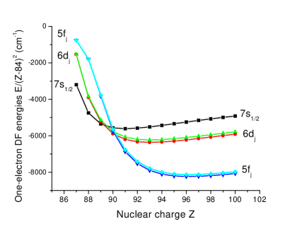
Figure 1: Dirac-Fock one-electron energies ($E/(Z-84)^{2}$ in cm^-1) for the $5f_{j}$, $6d_{j}$, and $7s_{1/2}$ states of Fr-like ions as functions of $Z$.

Relativistic Hartree-Fock and Dirac-Fock atomic structure codes were used in Ref. Biémont et al. (2004) to perform calculations of radiative transition rates and oscillator strengths for a limited number of transitions using the energies given by Blaise and Wyart , where experimental values were given for the $7p$, $8p$, $nd$ (with $n$ =10–33), and $ns$ (with $n$ =12–31) levels of neutral Fr, for 24 levels for Fr-like Th, and for seven levels of Fr-like Ac and U. Adopted energy level values in the $ns$, $np$, and $nd$ ($n\leq$ 30) series of neutral francium were presented by Biémont et al. (1998). Experimental measurements of energy levels of the $8s$ and $7d$ states in Fr I were reported recently in Refs. Simsarian et al. (1999); Grossman et al. (2000a). The experimental energies of 13 levels of Fr-like Ra were reported in the NIST compilation web .

Lifetime measurements for neutral francium were presented in Refs. Zhao et al. (1997); Simsarian et al. (1998); Grossman et al. (2000b); Aubin et al. (2003); Gomez et al. (2005) for the $7p$, $6d$, $9s$, and $8s$ levels. In those papers, experimental measurements were compared with ab-initio calculations performed by Johnson et al. (1996), Dzuba et al. (1995, 2001), Safronova et al. (1999), and Safronova and Johnson (2000). Third-order many-body perturbation theory was used in Ref. Johnson et al. (1996) to obtain the E1 transition amplitude for neutral alkali-metal atoms. The correlation potential method and the Feynman diagram technique were used in Refs. Dzuba et al. (1995, 2001) to calculate E1 matrix elements in neutral francium and Fr-like radium. Atomic properties of Th IV ion were studied by  Safronova et al. (2006) using a relativistic all-order method.

The present third-order calculations of excitation energies of the $7s$, $7p$, $6d$, and $5f$ states in Fr-like ions with nuclear charges $Z=87-100$ start from a closed-shell Dirac-Fock potential for the 86 electron radon-like core. We note that Th IV is the first ion in the francium isoelectronic sequence with a [Rn]$5f_{5/2}$ ground state instead of the [Rn]$7s_{1/2}$ ground state as for Fr I, Ra II, and Ac III. Correlation corrections become very large for such systems as was demonstrated by Savukov et al. (2003), where the ratio of the second-order and DF removal energies for the [Xe]$4f_{5/2}$ ground state in Ce IV and Pr V were 18% and 11%, respectively.

In the present paper, dipole matrix elements are calculated using both relativistic many-body perturbation theory, complete through third-order, and the relativistic all-order method restricted to single and double (SD) excitations. Such calculations permit one to investigate the convergence of perturbation theory and estimate the theoretical error in predicted data. To obtain lifetime predictions, multipole matrix elements for $7s-6d$, $7s-5f$ and $5f_{5/2}\ -5f_{7/2}$ transitions are also evaluated. Additionally, scalar polarizabilities for the $7s_{1/2}$ ground state in Fr I, Ra II, and Ac III are calculated using relativistic third-order and SD methods. Finally, scalar polarizabilities of the $5f_{5/2}$ ground state of Fr-like ions with nuclear charge $Z$ = 91–100 are calculated in second-order MBPT.

Table 1: Zeroth-order (DF), second-, and third-order Coulomb correlation energies $E^{(n)}$, single-double Coulomb energies $E^{\text{{SD}}}$, $E^{(3)}_{\text{{extra}}}$, first-order Breit and second-order Coulomb-Breit corrections $B^{(n)}$ to the energies of Fr-like systems. The total energies are $E^{(3)}_{\text{ tot}}=E^{(0)}+E^{(2)}+E^{(3)}+B^{(1)}+B^{(2)}$ + $E_{LS}$, $E^{\text{SD}}_{\text{tot}}=E^{(0)}+E^{\text{{SD}}}+E^{(3)}_{\text{{extra}}}+B^{(1)}+B^{(2)}$ + $E_{LS}$. Units: cm^-1.

$nlj$	$E^{(0)}$	$E^{(2)}$	$E^{(3)}$	$B^{(1)}$	$B^{(2)}$	$E_{LS}$	$E^{(3)}_{\text{ tot}}$	$E^{\text{{SD}}}$	$E^{(3)}_{\text{{extra}}}$	$E^{\text{{SD}}}_{\text{ tot}}$
Fr I, $Z$ = 87
$7s_{1/2}$	-28767	-4763	1737	67	-131	13	-31845	-4658	724	-32753
$7p_{1/2}$	-18855	-1847	546	30	-35	0	-20162	-1991	255	-20597
$7p_{3/2}$	-17655	-1346	391	19	-30	0	-18621	-1433	184	-18915
$6d_{3/2}$	-13807	-2424	711	19	-62	0	-15563	-3180	326	-16990
$6d_{5/2}$	-13924	-2240	616	15	-61	0	-15594	-2854	288	-16744
$8s_{1/2}$	-12282	-1053	396	17	-32	2	-12952	-925	162	-13058
$8p_{1/2}$	-9240	-554	171	10	-13	0	-9625	-551	77	-9716
$8p_{3/2}$	-8811	-421	128	7	-11	0	-9108	-421	58	-9178
$7d_{3/2}$	-7724	-981	298	10	-30	0	-8427	-991	132	-8604
$7d_{5/2}$	-7747	-860	244	7	-28	0	-8384	-856	109	-8515
Ra II, $Z$ = 88
$7s_{1/2}$	-75898	-7529	2896	147	-250	33	-80634	-6692	1152	-81508
$6d_{3/2}$	-62356	-8727	2764	155	-398	0	-68562	-8042	1152	-69488
$6d_{5/2}$	-61592	-7537	2202	114	-360	0	-67174	-7034	926	-67947
$7p_{1/2}$	-56878	-4182	1370	102	-109	0	-59698	-4027	587	-60326
$7p_{3/2}$	-52906	-3130	1011	63	-90	0	-55053	-3020	433	-55519
$5f_{5/2}$	-28660	-2563	824	11	-63	0	-30452	-4438	371	-32780
$5f_{7/2}$	-28705	-2491	784	8	-61	0	-30466	-4159	353	-32564
Ac III, $Z$ = 89
$7s_{1/2}$	-133640	-9552	3739	233	-357	58	-139519	-8192	1456	-140442
$6d_{3/2}$	-130697	-11506	3639	296	-659	0	-138927	-10036	1479	-139617
$6d_{5/2}$	-128322	-10002	2902	218	-600	0	-135804	-8884	1186	-136401
$5f_{5/2}$	-95668	-26451	9684	403	-1785	0	-113818	-23325	3952	-116424
$5f_{7/2}$	-94161	-24695	8837	289	-1658	0	-111387	-22100	3607	-114022
$7p_{1/2}$	-106328	-6202	2118	193	-189	0	-110409	-5688	874	-111139
$7p_{3/2}$	-98868	-4745	1597	119	-157	0	-102054	-4380	659	-102626
Th IV, $Z$ = 90
$5f_{5/2}$	-206606	-32100	11739	704	-2747	0	-229010	-26327	4672	-230304
$5f_{7/2}$	-203182	-30549	10954	521	-2616	0	-224872	-25252	4361	-226168
$6d_{3/2}$	-211799	-13258	4129	438	-880	0	-221370	-11422	1663	-222000
$6d_{5/2}$	-207574	-11608	3300	326	-807	0	-216364	-10208	1337	-216927
$7s_{1/2}$	-200273	-11204	4402	325	-458	89	-207119	-9455	1697	-208075
$7p_{1/2}$	-165095	-7991	2782	298	-272	0	-170278	-7147	1125	-171091
$7p_{3/2}$	-153572	-6213	2124	184	-226	1	-157703	-5619	861	-158372
Pa V, $Z$ = 91
$5f_{5/2}$	-336671	-34071	12323	953	-3390	0	-360855	-27589	4831	-361865
$5f_{7/2}$	-331505	-32627	11592	713	-3255	0	-355081	-26571	4544	-356073
$6d_{3/2}$	-303549	-14627	4452	586	-1082	0	-314221	-12604	1795	-314854
$6d_{5/2}$	-297300	-12880	3556	438	-999	0	-307185	-11354	1446	-307768
$7s_{1/2}$	-274949	-12646	3359	425	-557	126	-284242	-10606	1348	-284212
$7p_{1/2}$	-232148	-9630	2566	417	-356	0	-239151	-8533	1040	-239580
$7p_{3/2}$	-216015	-7600	4939	258	-297	1	-218715	-6925	1900	-221079
U VI, $Z$ = 92
$5f_{5/2}$	-481613	-35163	12554	1194	-3929	0	-506958	-28393	4876	-507866
$5f_{7/2}$	-474700	-33781	11863	898	-3789	0	-499509	-27398	4604	-500385
$6d_{3/2}$	-404911	-15830	4675	742	-1275	0	-416599	-13737	1908	-417273
$6d_{5/2}$	-396467	-14000	3718	557	-1181	0	-407374	-12472	1538	-408025
$7s_{1/2}$	-357141	-13966	5366	533	-655	173	-365690	-11752	2079	-366763
$7p_{1/2}$	-306870	-11224	3742	548	-442	0	-314245	-10135	1541	-315358
$7p_{3/2}$	-285578	-9134	2452	338	-369	2	-292289	-10236	1173	-294669

Table 2: The total third-order $E^{(3)}_{\text{ tot}}$ and all-order $E^{\text{SD}}_{\text{tot}}$ results for Fr-like ions are compared with experimental energies $E_{\text{{expt}}}$ Blaise and Wyart , $\delta E$ = $E_{\text{tot}}$ - $E_{\text{{expt}}}$. The energies are given relative to the ground state to facilitate comparison with experiment. Units: cm^-1

$nlj$	$E^{(3)}_{\text{ tot}}$	$E^{\text{{SD}}}_{\text{ tot}}$	$E_{\text{{expt}}}$	$\delta E^{(3)}$	$\delta E^{\text{{SD}}}$
Fr I, $Z$ = 87
$7s_{1/2}$	0	0	0	0	0
$7p_{1/2}$	11683	12156	12237	-554	-81
$7p_{3/2}$	13224	13838	13924	-700	-86
$6d_{3/2}$	16282	16048	16230	52	-192
$6d_{5/2}$	16251	16217	16430	-179	-213
$8s_{1/2}$	18893	19695	19733	-840	-38
$8p_{1/2}$	22220	23037	23113	-893	-76
$8p_{3/2}$	22737	23575	23658	-921	-83
$7d_{3/2}$	23418	24149	24245	-827	-96
$7d_{5/2}$	23461	24238	. 24333	-872	-95
Ra II, $Z$ = 88
$7s_{1/2}$	0	0	0	0	0
$6d_{3/2}$	12072	12020	12084	-12	-64
$6d_{5/2}$	13460	13561	13743	-283	-182
$7p_{1/2}$	20936	21182	21351	-415	-169
$7p_{3/2}$	25581	25989	26209	-628	-220
$5f_{5/2}$	50182	48728	48988	1194	-260
$5f_{7/2}$	50168	48944	49272	896	-328
Ac III, $Z$ = 89
$7s_{1/2}$	0	0	0	0	0
$6d_{3/2}$	592	825	801	-209	24
$6d_{5/2}$	3715	4041	4204	-488	-163
$5f_{5/2}$	25701	24018	23454	2247	564
$5f_{7/2}$	28132	26420	26080	2052	340
$7p_{1/2}$	29110	29303	29466	-356	-163
$7p_{3/2}$	37465	37816	38063	-598	-247
Th IV, $Z$ = 90
$5f_{5/2}$	0	0	0	0	0
$5f_{7/2}$	4138	4136	4325	-187	-190
$6d_{3/2}$	7640	8304	9193	-1553	-889
$6d_{5/2}$	12646	13377	14486	-1841	-1109
$7s_{1/2}$	21891	22229	23131	-1240	-901
$7p_{1/2}$	58732	59213	60239	-1507	-1026
$7p_{3/2}$	71307	71932	73056	-1749	-1124
U VI, $Z$ = 92
$5f_{5/2}$	0	0	0	0	0
$5f_{7/2}$	7449	7481	7609	-160	-128
$6d_{3/2}$	90359	90593	91000	-641	-407
$6d_{5/2}$	99584	99841	100510	-926	-669
$7s_{1/2}$	141268	141103	141447	-179	-344
$7p_{1/2}$	192713	191989	193340	-627	-832
$7p_{3/2}$	214669	211747	215886	-1217	-2689

II Third-order and all-order MBPT calculations of energies

We start from the “no-pair” Hamiltonian Sucher (1980)

$$H=H_{0}+V_{I}\,,$$ (1)

where $H_{0}$ and $V_{I}$ can be written in a second-quantized form as

$$H_{0}=\sum_{i}\varepsilon_{i}a_{i}^{\dagger}a_{i}\,,$$ (2)

$$V_{I}=\frac{1}{2}\sum_{ijkl}g_{ijkl}\ a_{i}^{\dagger}a_{j}^{\dagger}a_{l}a_{k}\,.$$ (3)

Negative-energy (positron) states are excluded from the sums. The quantities $\varepsilon_{i}$ are eigenvalues of the one-electron Dirac-Fock equations with a frozen core and $g_{ijkl}$ is a two-particle Coulomb matrix element. Our calculations start from a $V^{N-1}$ DF potential for a closed-subshell radon-like ion.

The all-order single-double (SD) method was discussed previously in Refs. Blundell et al. (1989); Liu ; Blundell et al. (1991); Safronova et al. (1998, 1999); Safronova and Johnson (2004). Briefly, we represent the wave function $\Psi_{v}$ of an atom with one valence electron atom as $\Psi_{v}\cong\Psi_{v}^{\rm SD}$ with

$$\Psi_{v}^{\rm SD}=\left[1+\sum_{ma}\rho_{ma}a_{m}^{\dagger}a_{a}+\frac{1}{2}\sum_{mnab}\rho_{mnab}a_{m}^{\dagger}a_{n}^{\dagger}a_{b}a_{a}\right.$$ (4)

$$\left.+\sum_{m\neq v}\rho_{mv}a_{m}^{\dagger}a_{v}+\sum_{mna}\rho_{mnva}a_{m}^{\dagger}a_{n}^{\dagger}a_{a}a_{v}\right]\!\!\Phi_{v},$$

where $\Phi_{v}$ is the lowest-order atomic wave function, which is taken to be the frozen-core DF wave function of a state $v$. Substituting the wave function $\Psi_{v}^{\rm SD}$ into the many-body Schrödinger equation, with Hamiltonian given by the Eqs. (1–3), one obtains the coupled equations for the single- and double-excitation coefficients $\rho_{mv}$, $\rho_{ma}$, $\rho_{mnva}$, and $\rho_{mnab}$. The coupled equations for the excitation coefficients are solved iteratively. We use the resulting excitation coefficients to evaluate multipole matrix elements and hyperfine constants. This method includes contribution of important classes of MBPT corrections to all orders.

The SD valence $E_{v}^{\rm SD}$ energy does not include a all third-order MBPT corrections. The missing part of the third-order contribution, $E_{\rm extra}^{(3)}$, is written out in Ref. Safronova et al. (1998) and must be calculated separately. We use our third-order energy code to separate out $E_{\rm extra}^{(3)}$ and add it to the $E_{v}^{\rm SD}$. For notational simplicity, we drop the index $v$ in the designations in the text and tables below.

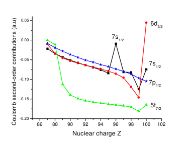
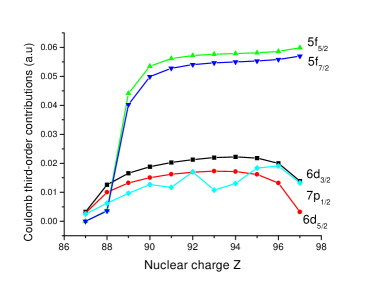
Figure 2: Coulomb second and third-order energies as functions of $Z$ for the $5f_{j}$, $6d_{j}$, $7s_{1/2}$, and $7p_{1/2}$ states in Fr-like ions.

Results of our energy calculations for low-lying states of Fr I–U VI are summarized in Table 1. Columns 2–7 of Table 1 give the lowest-order DF energies $E^{(0)}$, second- and third-order Coulomb correlation energies, $E^{(2)}$ and $E^{(3)}$, first-order Breit contribution $B^{(1)}$, second-order Coulomb-Breit $B^{(2)}$ corrections, and the Lamb shift contribution, $E_{\rm LS}$. The sum of these six contributions is our final third-order MBPT result $E^{(3)}_{\rm tot}$ listed in the eighth column. First-order Breit energies (column $B^{(1)}$ of Table 1) include retardation, whereas the second-order Coulomb-Breit energies (column $B^{(2)}$ of Table 1) are evaluated using the unretarded Breit operator. We list all-order SD energies in the column labelled $E^{\text{{SD}}}$ and the part of the third-order energies omitted in the SD calculation in column $E^{(3)}_{\text{{extra}}}$. We note that $E^{\text{{SD}}}$ includes $E^{(2)}$, part of $E^{(3)}$, and dominant higher-order corrections. The sum of the six terms $E^{(0)}$, $E^{\text{{SD}}}$, $E^{(3)}_{\text{{extra}}}$, $B^{(1)}$, $B^{(2)}$, and $E_{\rm LS}$ gives the final all-order results $E^{\text{{SD}}}_{\rm tot}$ listed in the eleventh column of the table.

As expected, the largest correlation contribution to the valence energy comes from the second-order term, $E^{(2)}$. This term is simple to calculate in comparison with $E^{(3)}$ and $E^{\rm SD}$ terms. Thus, we calculate the $E^{(2)}$ term with higher numerical accuracy than $E^{(3)}$ and $E^{\rm SD}$. The second-order energy $E^{(2)}$ includes partial waves up to $l_{\text{max}}=8$ and is extrapolated to account for contributions from higher partial waves (see, for example, Refs. Safronova et al. (1996, 1997)). As an example of the convergence of $E^{(2)}$ with the number of partial waves $l$, we consider the $5f_{5/2}$ state in U VI. Calculations of $E^{(2)}$ with $l_{\text{max}}$ = 6 and 8 yield $E^{(2)}(5f_{5/2})$ = -33598 and -347559 cm^-1, respectively. Extrapolation of these calculations yields -35163 and -35227 cm^-1, respectively. Therefore, we estimate the numerical uncertainty of $E^{(2)}(5f_{5/2})$ to be 64 cm^-1. This is the largest contribution from the higher partial waves, since the numerical uncertainty of $E^{(2)}(6d)$ is equal to 34 cm^-1, and the numerical uncertainty of $E^{(2)}(7s)$ is equal to 1 cm^-1. The numerical uncertainty of the second-order energy calculation for all other states ranges from 1 cm^-1 to 5 cm^-1. We use $l_{\text{max}}$ = 6 in our third-order and all-order calculations, owing to the complexity of these calculations. Therefore, we use our high-precision calculation of $E^{(2)}$ described above to account for the contributions of the higher partial waves, i.e. we replace $E^{(2)}$[$l_{\text{max}}$ = 6] with the final high-precision second-order value $E^{(2)}_{\rm final}$. The contribution $E^{(3)}_{\text{{extra}}}$ given in Table 1 accounts for that part of the third-order MBPT correction not included in the SD energy. The values of $E^{(3)}_{\text{{extra}}}$ are quite large and including this term is important.

We find that the correlation corrections to energies are especially large for $5f$ states. For example, $E^{(2)}$ is about 15% of $E^{(0)}$ and $E^{(3)}$ is about 36% of $E^{(2)}$ for $5f$ states. Despite the evident slow convergence of the perturbation theory expansion, the $5f$ energy from the third-order MBPT calculation is within 0.9% of the measured energy. The correlation corrections are so large for the $5f$ states that inclusion of correlation leads to the different ordering of states using the DF and $E^{(3)}_{\text{ tot}}$ energies. If we consider only DF energies the $6d_{3/2}$ appears to be the ground state for Th IV, but the full correlation shows that the $5f_{5/2}$ is the ground state. The correlation corrections are much smaller for all other states; the ratios of $E^{(0)}$ and $E^{(2)}$ are equal to 6%, 5%, and 2% for the $6d$, $7s$, and $10s$ states, respectively.

The third-order and all-order results are compared with experimental values in Table 2. The energies are given relative to the ground state to facilitate comparison with experiment. Experimental energies for Fr I, Ac III, Th IV, and U VI are taken from Blaise and Wyart and energies of Fr-like Ra are taken from the NIST compilation web . Differences of our third-order and all-order calculations with experimental data, $\delta E^{(3)}=E^{(3)}_{\rm tot}-E_{\text{{expt}}}$ and $\delta E^{\text{SD}}=E^{\text{{SD}}}_{\rm tot}-E_{\text{{expt}}}$, respectively, are given in the two final columns of Table 2. In general, the SD results agree better with the experimental values than the third-order MBPT values. Exceptions are the cases where the third-order fortuitously give results that are close to experimental values. Comparison of results from two last columns of Table 2 shows that the ratio of $\delta E^{(3)}$ and $\delta E^{\text{{SD}}}$ is about three for the $5f$ states. As expected, including correlation to all orders led to significant improvement of the results. Better agreement of all-order energies with experiment demonstrates the importance of the higher-order correlation contributions.

Below, we describe a few numerical details of the calculation. We use the B-spline method described Johnson et al. (1988a) to generate a complete set of basis DF wave functions for use in the evaluation of the MBPT expressions. We use 50 splines of order $k=8$ for each angular momentum. The basis orbitals are constrained to a spherical cavity of radius $R$ = 90–30 a.u for Fr I–U VI. The cavity radius is chosen large enough to accommodate all $nl_{j}$ orbitals considered here and small enough that 50 splines can approximate inner-shell DF wave functions with good precision. We use 40 out 50 basis orbitals for each partial wave in our third-order and all-order energy calculations, since contributions from the highest-energy orbitals are negligible.

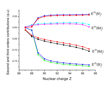
Figure 3: Coulomb second- and third-order energies as functions of $Z$ for the $5f_{j}$ and $6d_{j}$ states in Fr-like ions.

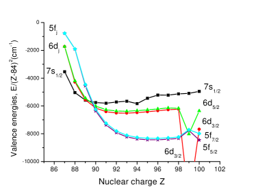
Figure 4: Valence removal energies ($E/(Z-84)^{2}$ in cm^-1) as functions of $Z$ for the $5f_{j}$, $6d_{j}$, and $7s_{1/2}$ states in Fr-like ions.

II.1 $Z$ dependence of energies in Fr-like ions

In Fig. 2, we illustrate the $Z$-dependence of the second and third-order energy corrections $E^{(n)}$ for the valence $7s$, $7p$, $6d$, and $5f$ states of Fr-like ions. The second-order energy $E^{(2)}$ is a smooth function of $Z$ for the $7p_{1/2}$ and $5f_{7/2}$ states, but exhibits a few sharp features for the $7s_{1/2}$ and $6d_{5/2}$ states. These very strong irregularities occur for the $7s_{1/2}$ state $Z$=96, 99 and $6d_{5/2}$ state for $Z$=99 and are explained by accidentally small energy denominators in the MBPT expressions for the correlation corrections to the energy. The third-order energy $E^{(3)}$ is a smooth function of $Z$ for the $6d$ and $5f$ states, but exhibits a similar sharp features for the $7p_{1/2}$ state. Most of the sharp features for the $6d_{j}$ and $7p_{j}$ states occur at very high values of $Z$, $Z>$ 97. Comparison of the $E^{(2)}$ and $E^{(3)}$ corrections for the $6d$ and $5f$ states is illustrated by Fig. 3. This figure shows also the smooth dependence of second- and third-order corrections to the $6d_{5/2}-6d_{3/2}$ and $5f_{7/2}-5f_{5/2}$ fine-structure intervals.

The total $E^{(3)}_{\text{ tot}}$ energies divided by $(Z-84)^{2}$ in Fr-like ions are shown in Fig. 4. We plot the five energy levels for the $7s_{1/2}$, $6d_{j}$, and $5f_{j}$ states. The $Z$-dependence of $E^{(3)}_{\text{ tot}}$ is smooth up to very high $Z$. Irregularities observed in Fig. 4 for high $Z$ are explained by vanishing energy denominators in MBPT expressions for correlation corrections.

Table 3: Reduced electric-dipole matrix elements in Fr-like ions calculated to first, second, third, and all orders of MBPT.

Transition		$Z^{({\rm DF})}$	$Z^{({\rm DF}+2)}$	$Z^{({\rm DF}+2+3)}$	$Z^{\text{{(SD)}}}$	Transition		$Z^{({\rm DF})}$	$Z^{({\rm DF}+2)}$	$Z^{({\rm DF}+2+3)}$	$Z^{\text{{(SD)}}}$
Fr I, $Z$ = 87						Th IV, $Z$ = 90
$7s_{1/2}$	$7p_{1/2}$	5.1438	4.7412	4.1362	4.2641	$7s_{1/2}$	$7p_{1/2}$	2.8994	2.3748	2.3669	2.4196
$7s_{1/2}$	$7p_{3/2}$	7.0903	6.6001	5.6451	5.8619	$7s_{1/2}$	$7p_{3/2}$	3.9933	3.3399	3.2930	3.3677
$6d_{3/2}$	$7p_{1/2}$	9.2216	8.7781	7.1945	7.0276	$6d_{3/2}$	$7p_{1/2}$	2.5465	2.1374	2.0723	2.1220
$6d_{3/2}$	$7p_{3/2}$	4.2832	4.1100	3.3108	3.2217	$6d_{3/2}$	$7p_{3/2}$	0.9963	0.8784	0.8270	0.8488
$6d_{5/2}$	$7p_{3/2}$	12.8041	12.2858	10.1204	9.9456	$6d_{5/2}$	$7p_{3/2}$	3.1975	2.8348	2.7006	2.7549
$6d_{3/2}$	$5f_{5/2}$	11.4529	11.3002	6.7352	6.9611	$6d_{3/2}$	$5f_{5/2}$	2.4281	1.4501	1.3367	1.5295
$6d_{5/2}$	$5f_{5/2}$	3.0143	2.9714	1.9006	1.9515	$6d_{5/2}$	$5f_{5/2}$	0.6391	0.4070	0.3624	0.4116
$6d_{5/2}$	$5f_{7/2}$	13.4863	13.2942	8.5062	8.7332	$6d_{5/2}$	$5f_{7/2}$	2.9557	1.8844	1.7032	1.9190
Ra II, $Z$ = 88						Pa V, $Z$ = 91
$7s_{1/2}$	$7p_{1/2}$	3.8766	3.3758	3.1793	3.2545	$7s_{1/2}$	$7p_{1/2}$	2.6267	2.1111	2.1365	2.1822
$7s_{1/2}$	$7p_{3/2}$	5.3395	4.7241	4.3881	4.5106	$7s_{1/2}$	$7p_{3/2}$	3.6173	2.9720	2.9750	3.0327
$6d_{3/2}$	$7p_{1/2}$	4.4462	3.9314	3.3975	3.5659	$6d_{3/2}$	$7p_{1/2}$	2.1785	1.8079	1.7817	1.8152
$6d_{3/2}$	$7p_{3/2}$	1.8815	1.7070	1.4262	1.5117	$6d_{3/2}$	$7p_{3/2}$	0.8319	0.7327	0.7004	0.7119
$6d_{5/2}$	$7p_{3/2}$	5.8616	5.3340	4.6240	4.8232	$6d_{5/2}$	$7p_{3/2}$	2.6895	2.3817	2.2936	2.3185
$6d_{3/2}$	$5f_{5/2}$	5.3548	4.6786	4.5967	4.4491	$6d_{3/2}$	$5f_{5/2}$	1.9275	1.0904	1.0864	1.2092
$6d_{5/2}$	$5f_{5/2}$	1.4797	1.3062	1.3088	1.2465	$6d_{5/2}$	$5f_{5/2}$	0.5023	0.3061	0.2947	0.3241
$6d_{5/2}$	$5f_{7/2}$	6.6382	5.8609	5.8347	5.6357	$6d_{5/2}$	$5f_{7/2}$	2.3242	1.4102	1.3673	1.5020
Ac III, $Z$ = 89						U VI, $Z$ = 92
$7s_{1/2}$	$7p_{1/2}$	3.2787	2.7544	2.6859	2.7463	$7s_{1/2}$	$7p_{1/2}$	2.4165	1.9138	1.9562	1.9599
$7s_{1/2}$	$7p_{3/2}$	4.5157	3.8665	3.7271	3.8176	$7s_{1/2}$	$7p_{3/2}$	3.3271	2.6952	2.7168	2.2449
$6d_{3/2}$	$7p_{1/2}$	3.1529	2.6942	2.5241	2.6048	$6d_{3/2}$	$7p_{1/2}$	1.9249	1.5837	1.5688	1.5613
$6d_{3/2}$	$7p_{3/2}$	1.2726	1.1300	1.0275	1.0662	$6d_{3/2}$	$7p_{3/2}$	0.7202	0.6353	0.6054	0.4963
$6d_{5/2}$	$7p_{3/2}$	4.0423	3.6067	3.3438	3.4383	$6d_{5/2}$	$7p_{3/2}$	2.3417	2.0760	1.9887	1.6018
$6d_{3/2}$	$5f_{5/2}$	3.5764	2.3879	1.7460	2.1624	$6d_{3/2}$	$5f_{5/2}$	1.6274	0.8798	0.9034	0.9974
$6d_{5/2}$	$5f_{5/2}$	0.9577	0.6708	0.4760	0.5877	$6d_{5/2}$	$5f_{5/2}$	0.4209	0.2479	0.2470	0.2674
$6d_{5/2}$	$5f_{7/2}$	4.4148	3.1076	2.2956	2.7539	$6d_{5/2}$	$5f_{7/2}$	1.9492	1.1353	1.1293	1.2293

Table 4: Comparison of length [L] and velocity [V] results for reduced electric-dipole matrix elements in first, second, and third orders of perturbation theory in Fr-like systems with $Z$ = 87–92.

Ion	$Z^{({\rm DF})}$		$Z^{({\rm DF}+2)}$		$Z^{({\rm DF}+2+3)}$		$Z^{({\rm DF})}$		$Z^{({\rm DF}+2)}$		$Z^{({\rm DF}+2+3)}$
	$L$	$V$	$L$	$V$	$L$	$V$	$L$	$V$	$L$	$V$	$L$	$V$
$6d_{3/2}-5f_{5/2}$						$6d_{5/2}-5f_{7/2}$
87	11.4529	11.4002	11.2693	11.2693	7.8982	7.8972	13.4863	13.4022	13.2703	13.2703	9.6464	9.6455
88	5.3549	5.1362	4.7603	4.7603	4.4885	4.4839	6.6382	6.3283	5.9720	5.9720	5.7071	5.7056
89	3.5764	3.1632	2.6134	2.6134	0.5254	0.4982	4.4148	3.8730	3.3832	3.3831	0.8484	0.8576
90	2.4281	0.7698	1.6597	1.6595	2.8562	2.9000	2.9557	0.5609	2.1257	2.1255	3.3454	3.3138
91	1.9275	2.0349	1.2702	1.2702	1.4017	1.4122	2.3242	2.4373	1.6097	1.6097	1.7219	1.7100
92	1.6274	1.6199	1.0312	1.0312	1.0559	1.0613	1.9492	1.9305	1.2978	1.2978	1.3024	1.2943
$6d_{3/2}-7p_{1/2}$						$7s_{3/2}-7p_{3/2}$
87	9.2216	9.9449	8.7906	8.7906	6.8407	6.8365	7.0903	6.6425	6.6268	6.6268	5.9488	5.9486
88	4.4462	2.0213	3.9815	3.9816	3.8547	3.8589	5.3395	4.9435	4.7968	4.7969	4.5150	4.5148
89	3.1529	2.3683	2.7533	2.7533	2.6221	2.6238	4.5158	4.1785	3.9641	3.9641	3.8018	3.8016
90	2.5465	2.0531	2.1960	2.1961	2.1074	2.1084	3.9933	3.7030	3.4515	3.4516	3.3434	3.3432
91	2.1785	1.8158	1.8631	1.8631	1.7957	1.7964	3.6173	3.3638	3.0915	3.0915	3.0121	3.0119
92	1.9249	1.6384	1.6343	1.6344	1.5743	1.5748	3.3271	3.1029	2.8190	2.8190	2.7460	2.7458

Table 5: Wavelengths $\lambda$ (Å), weighted transition rates $gA$ (s^-1) and oscillator strengths $gf$ in Ac III, Th IV, and U VI. The SD data ($gA^{\mathrm{(SD)}}$ and $gf^{\mathrm{(SD)}}$) are compared with theoretical ($gA^{\mathrm{(RHF)}}$ and $gf^{\mathrm{(RHF)}}$) values given in Ref. Biémont et al. (2004). Numbers in brackets represent powers of 10.

Lower	Upper	$\lambda^{\text{{(expt)}}}$	$gA^{\mathrm{(SD)}}$	$gA^{\mathrm{(RHF)}}$	$gf^{\mathrm{(SD)}}$	$gf^{\mathrm{(RHF)}}$
Ac III, $Z$ = 89
$7s_{1/2}$	$7p_{3/2}$	2626.44	1.63[9]	1.55[9]	1.69[+0]	1.6[+0]
$6d_{3/2}$	$7p_{3/2}$	2682.90	1.19[8]	1.23[8]	1.29[-1]	1.3[-1]
$6d_{5/2}$	$7p_{3/2}$	2952.55	9.30[8]	8.23[8]	1.22[+0]	1.1[+0]
$7s_{1/2}$	$7p_{1/2}$	3392.78	3.91[8]	3.59[8]	6.75[-1]	6.2[-1]
$6d_{3/2}$	$7p_{1/2}$	3487.59	3.24[8]	2.75[8]	5.91[-1]	5.0[-1]
$6d_{3/2}$	$5f_{5/2}$	4413.09	1.10[8]	2.34[8]	3.22[-1]	6.9[-1]
$6d_{5/2}$	$5f_{7/2}$	4569.97	1.61[8]	3.02[8]	5.04[-1]	9.5[-1]
$6d_{5/2}$	$5f_{5/2}$	5193.21	4.99[6]	1.03[6]	2.02[-2]	4.2[-2]
Th IV, $Z$ = 90
$6d_{3/2}$	$7p_{3/2}$	1565.86	3.80[8]	4.08[8]	1.40[-1]	1.5[-1]
$6d_{5/2}$	$7p_{3/2}$	1707.37	3.09[9]	2.83[9]	1.35[+0]	1.2[+0]
$6d_{3/2}$	$7p_{1/2}$	1959.02	1.21[9]	1.04[9]	6.98[-1]	6.0[-1]
$7s_{1/2}$	$7p_{3/2}$	2003.00	2.86[9]	2.70[9]	1.72[+0]	1.6[+0]
$7s_{1/2}$	$7p_{1/2}$	2694.81	6.06[8]	5.55[8]	6.60[-1]	6.0[-1]
$5f_{5/2}$	$6d_{5/2}$	6903.05	1.04[6]	2.22[6]	7.45[-3]	1.6[-2]
$5f_{7/2}$	$6d_{5/2}$	9841.54	7.83[6]	1.53[7]	1.14[-1]	2.2[-1]
$5f_{5/2}$	$6d_{3/2}$	10877.55	3.68[6]	7.93[6]	6.53[-2]	1.4[-1]
U VI, $Z$ = 92
$6d_{3/2}$	$7p_{3/2}$	800.729	9.72[8]	1.72[9]	9.34[-2]	1.7[-1]
$6d_{5/2}$	$7p_{3/2}$	866.737	7.98[9]	1.26[10]	8.99[-1]	1.4[+0]
$6d_{3/2}$	$7p_{1/2}$	977.129	5.29[9]	4.87[9]	7.58[-1]	6.9[-1]
$5f_{5/2}$	$6d_{5/2}$	994.921	1.47[8]	3.51[8]	2.18[-2]	5.2[-2]
$5f_{7/2}$	$6d_{5/2}$	1076.40	2.46[9]	5.55[9]	4.26[-1]	9.5[-1]
$5f_{5/2}$	$6d_{3/2}$	1098.91	1.52[9]	3.64[9]	2.75[-1]	6.6[-1]
$7s_{1/2}$	$7p_{3/2}$	1343.39	4.21[9]	6.08[9]	1.14[+0]	1.7[+0]
$7s_{1/2}$	$7p_{1/2}$	1927.05	1.09[9]	1.03[9]	6.05[-1]	5.8[-1]

Table 6: Wavelengths $\lambda$ (Å), weighted transition rates $gA$ (s^-1) and oscillator strengths $gf$ in Fr I and Ra II. The SD data ($gA^{\mathrm{(SD)}}$ and $gf^{\mathrm{(SD)}}$) are compared with theoretical ($gA^{\mathrm{(RHF)}}$, $gf^{\mathrm{(RHF)}}$) values given in Ref. Biémont et al. (1998, 2004) and theoretical ($gA^{\mathrm{(MBPT)}}$, $gf^{\mathrm{(MBPT)}}$) values given in Ref. Dzuba et al. (2001). Numbers in brackets represent powers of 10.

Lower	Upper	$\lambda^{\text{{(expt)}}}$	$gA^{\mathrm{(SD)}}$	$gA^{\mathrm{(MBPT)}}$	$gA^{\mathrm{(RHF)}}$	$gf^{\mathrm{(SD)}}$	$gf^{\mathrm{(MBPT)}}$	$gf^{\mathrm{(RHF)}}$
Fr I, $Z$ = 87
$7s_{1/2}$	$7p_{3/2}$	7181.84	1.88[8]			1.45[+0]	1.46[+0]	1.5[+0]
$7s_{1/2}$	$7p_{1/2}$	8171.66	6.75[7]			6.76[-1]	6.84[-1]	6.5[-1]
$7p_{1/2}$	$7d_{3/2}$	8328.18	4.39[7]			4.57[-1]	4.40[-1]	6.9[-1]
$7p_{3/2}$	$7d_{5/2}$	9606.79	8.83[7]			1.22[+0]	1.18[+0]	1.1[+0]
$7p_{3/2}$	$7d_{3/2}$	9689.14	1.08[7]			1.52[-1]	1.49[-1]	1.2[-1]
$7p_{1/2}$	$8s_{1/2}$	13342.0	1.49[7]			3.99[-1]
$7p_{3/2}$	$8s_{1/2}$	17216.1	2.18[7]			9.70[-1]
Ra II, $Z$ = 88
$6d_{3/2}$	$5f_{5/2}$	2708.96	2.02[9]		1.59[9]	2.22[+0]		1.7[+0]
$6d_{5/2}$	$5f_{7/2}$	2813.76	2.89[9]		2.01[9]	3.43[+0]		2.4[+0]
$6d_{5/2}$	$5f_{5/2}$	2836.46	1.38[8]		9.80[7]	1.66[-1]		1.2[-1]
$7s_{1/2}$	$7p_{3/2}$	3814.42	7.42[8]	7.30[8]	7.14[8]	1.62[+0]	1.59[+0]	1.5[+0]
$7s_{1/2}$	$7p_{1/2}$	4682.28	2.09[8]	2.05[8]	1.93[8]	6.87[-1]	6.73[-1]	6.3[-1]
$6d_{3/2}$	$7p_{3/2}$	7077.95	1.30[7]	1.29[7]	1.27[7]	9.80[-2]	9.70[-2]	9.5[-2]
$6d_{5/2}$	$7p_{3/2}$	8019.70	9.13[7]	9.10[7]	7.85[7]	8.81[-1]	8.78[-1]	7.6[-1]
$6d_{3/2}$	$7p_{1/2}$	10788.2	2.05[7]	2.03[7]	1.79[7]	3.58[-1]	3.54[-1]	3.1[-1]

Table 7: Lifetimes ${\tau}$ in ns for the $nl$ levels for neutral francium. Our SD results are compared with experimental measurements presented in Ref. Simsarian et al. (1998) for the $7p_{j}$ levels, in Ref. Grossman et al. (2000b) for the $7d_{j}$ levels, and in Ref. Gomez et al. (2005) for the $8s_{1/2}$ level.

Level	$\tau^{(\rm SD)}$	$\tau^{(\rm expt)}$
$7p_{1/2}$	29.62	29.45$\pm$0.11
$7p_{3/2}$	21.28	21.02$\pm$0.11
$7d_{3/2}$	73.08	73.6$\pm$0.3
$7d_{5/2}$	67.93	67.7$\pm$2.9
$8s_{1/2}$	54.36	53.30$\pm$0.44

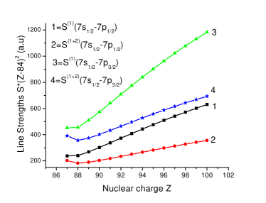
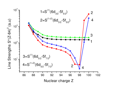
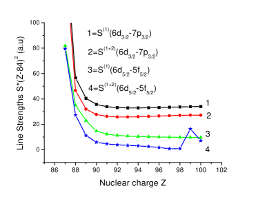
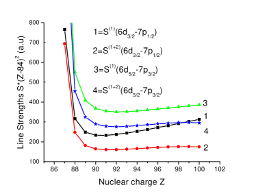
Figure 5: Line Strengths ($S\times(Z-84)^{2}$ in a.u) as functions of $Z$ in Fr-like ions.

III Electric-dipole matrix elements, oscillator strengths, transition rates, and lifetimes in Fr-like ions

III.1 Electric-dipole matrix elements

The matrix element of a one-particle operator $Z$ is given by Blundell et al. (1989)

$$Z_{wv}=\frac{\left\langle\Psi_{w}\right|Z\left|\Psi_{v}\right\rangle}{\sqrt{\left\langle\Psi_{v}|\Psi_{v}\right\rangle\left\langle\Psi_{w}|\Psi_{w}\right\rangle}}\,,$$ (5)

where $\Psi_{v}$ is the exact wave function for the many-body “no-pair” Hamiltonian $H$. In MBPT, we expand the many-electron wave function $\Psi_{v}$ in powers of $V_{I}$ as

$$\left|\Psi_{v}\right\rangle=\left|\Psi_{v}^{(0)}\right\rangle+\left|\Psi_{v}^{(1)}\right\rangle+\left|\Psi_{v}^{(2)}\right\rangle+\left|\Psi_{v}^{(3)}\right\rangle+\cdots\,.$$ (6)

The denominator in Eq. (5) arises from the normalization condition that contributes starting from third order Blundell et al. (1987). In the lowest order, we find

$$Z_{wv}^{(1)}=\left\langle\Psi_{w}^{(0)}\right|Z\left|\Psi_{v}^{(0)}\right\rangle=z_{wv}\,,$$ (7)

where $z_{wv}$ is the corresponding one-particle matrix element Johnson et al. (1995). Since $\Psi_{w}^{(0)}$ is a DF function we designate $Z^{(1)}$ by $Z^{(\rm DF)}$ below.

The second-order Coulomb correction to the transition matrix element in the DF case with $V^{N-1}$ potential is given by Johnson et al. (1996)

$$Z_{wv}^{(2)}=\sum_{na}\frac{z_{an}(g_{wnva}-g_{wnav})}{\varepsilon_{a}+\varepsilon_{v}-\varepsilon_{n}-\varepsilon_{w}}+\sum_{na}\frac{(g_{wavn}-g_{wanv})z_{na}}{\varepsilon_{a}+\varepsilon_{w}-\varepsilon_{n}-\varepsilon_{v}}\,.$$ (8)

Second-order Breit corrections are obtained from Eq. (8) by changing $g_{ijkl}$ to $b_{ijkl}$, where $b_{ijkl}$ is the matrix element of the Breit operator given in  Johnson et al. (1988b).

In the all-order SD calculation, we substitute the all-order SD wave function $\Psi_{v}^{\rm SD}$ into the matrix element expression given by Eq. (5) and obtain the expression  Blundell et al. (1989)

$$Z_{wv}^{(\rm SD)}=\frac{z_{wv}+Z^{(a)}+\cdots+Z^{(t)}}{\sqrt{(1+N_{w})(1+N_{v})}}\,,$$ (9)

where $z_{wv}$ is the lowest-order (DF) matrix element given by Eq. (7), and the terms $Z^{(k)}$, $k=a\cdots t$ are linear or quadratic functions of the excitation coefficients introduced in Eq. (4). The normalization terms $N_{w}$ are quadratic functions of the excitation coefficients. As a result, certain sets of many-body perturbation theory terms are summed to all orders. In contrast to the energy, all-order SD matrix elements contain the entire third-order MBPT contribution.

The calculation of the transition matrix elements provide another test of the quality of atomic-structure calculations and another measure of the size of correlation corrections. Reduced electric-dipole matrix elements between low-lying states of Fr-like systems with $Z$ = 87–92 calculated in various approximations are presented in Table 3.

Our calculations of the reduced matrix elements in the lowest, second, and third orders are carried out following the method described above. The lowest order DF value is obtained from Eq. (7). The values $Z^{({\rm DF}+2)}$ are obtained as the sum of the second-order correlation correction $Z^{(2)}$ given by Eq. (8) and the DF matrix elements $Z^{(\rm DF)}$. The second-order Breit corrections $B^{(2)}$ are rather small in comparison with the second-order Coulomb correction $Z^{(2)}$ (the ratio of $B^{(2)}$ to $Z^{(2)}$ is about 0.2%–2%).

The third-order matrix elements $Z^{({\rm DF}+2+3)}$ include the DF values, the second-order $Z^{(2)}$ results, and the third-order $Z^{(3)}$ correlation correction. $Z^{(3)}$ includes random-phase-approximation terms (RPA) iterated to all orders  Johnson et al. (1996).

We find correlation corrections $Z^{(2+3)}$ to be very large, 10-25%, for many cases. All results given in Table 3 are obtained using length form of the matrix elements. Length-form and velocity-form matrix elements differ typically by 5–20% for the DF matrix elements and 2–5 % for the second-order matrix elements in these calculations.

Electric-dipole matrix elements evaluated in the all-order SD approximation are given in columns labeled $Z^{\text{(SD)}}$ (Eq. (9)) of Table 3. The SD matrix elements $Z^{\text{(SD)}}$ include $Z^{(3)}$ completely, along with important fourth- and higher-order corrections. The fourth-order corrections omitted from the SD matrix elements were discussed recently by Derevianko and Emmons (2002). The $Z^{\text{{(SD)}}}$ values are smaller than the $Z^{({\rm DF}+2)}$ values and larger than the $Z^{({\rm DF}+2+3)}$ values for all transitions given in Table 3.

In Fig. 5, we illustrate the $Z$-dependences of the line strengths for the $7s_{1/2}-7p_{j}$, $6d_{j}-7p_{j^{\prime}}$, and $6d_{j}-5f_{j^{\prime}}$ transitions. Two sets of line strengths values $S^{(1)}$ and $S^{(1+2)}$ are presented for each transition. The values of $S^{(1)}$ and $S^{(1+2)}$ are obtained as $(Z^{(\rm DF)})^{2}$ and $(Z^{(\rm DF+2)})^{2}$, respectively. It should be noted that the values are scaled by $(Z-84)^{2}$ to provide better presentation of the line strengths. The difference between $S^{(1)}$ and $S^{(1+2)}$ curves increases with increasing $Z$; for the $7s_{1/2}-7p_{1/2}$ transition, the ratio of the second-order ($S^{(1+2)}$ - $S^{(1)}$) and the first-order ($S^{(1)}$) contributions is equal to 15% and 37% for $Z$ =87 and 92, respectively.

III.2 Form-independent third-order transition amplitudes

We calculate electric-dipole reduced matrix elements using the form-independent third-order perturbation theory developed by Savukov and Johnson in Ref. Savukov and Johnson (2000). Previously, a good precision of this method has been demonstrated for alkali-metal atoms. In this method, form-dependent “bare” amplitudes are replaced with form-independent random-phase approximation (“dressed”) amplitudes to obtain form-independent third-order amplitudes to some degree of accuracy. As in the case of the third-order energy calculation, a limited number of partial waves with $l_{\max}<7$ is included. This restriction is not very important for considered here ions because third-order correction is quite small, but it gives rise to some loss of gauge invariance. The gauge independence serves as a check that no numerical problems occurred.

Length and velocity-form matrix elements from DF, second-order (RPA), and third-order calculations are given in Table 4 for the limited number of transitions in Fr-like systems with $Z$ = 87–100. The $Z^{(\rm DF)}$ values differ in $L$ and $V$ forms by 2–15 % for the $p-s$ transitions. The very large $L-V$ difference (by a factor of 2–3) is observed in the $Z^{(\rm DF)}$ values for $d-f$ transitions as illustrated in Table 4. The second-order RPA contribution removes this difference in $L-V$ values, and the $L$ and $V$ columns with the $Z^{(\rm DF+2)}$ headings are almost identical. There are, however, small $L-V$ differences (0.002%–0.2%) in the third-order matrix elements. These remaining small differences can be explained by limitation in the number of partial waves taken into account in the $l_{max}$ in the third-order matrix element evaluations that we already discussed in the previous section describing the energy calculations.

III.3 Oscillator strengths, transition rates, and lifetimes

We calculate oscillator strengths and transition probabilities for the eight $7s-7p$, $7p-6d$, and $6d-5f$ electric-dipole transitions in Ra II, Ac III, Th IV, U VI and for the seven $7s-7p$, $7p-7d$, and $7p-8s$ electric-dipole transitions in Fr I. Wavelengths $\lambda$ (Å), weighted transition rates $gA$ (s^-1), and oscillator strengths $gf$ in Ac III, Th IV, U VI are given in Table 5 for Ac III, Th IV, U VI ions and in Table 6 for Ra II and Fr I.

The SD data ($gA^{\mathrm{(SD)}}$ and $gf^{\mathrm{(SD)}}$) are compared with theoretical ($gA^{\mathrm{(RHF)}}$ and $gf^{\mathrm{(RHF)}}$) results from Ref. Biémont et al. (2004). The experimental energies were used to calculate the $gA^{\mathrm{(SD)}}$, $gf^{\mathrm{(SD)}}$, $gA^{\mathrm{(RHF)}}$, and $gf^{\mathrm{(RHF)}}$. Therefore, we really compare the values of the electric-dipole matrix elements. The SD and RHF results for $s-p$ and $p-d$ transitions disagree by about 6–25 % with exception of the $6d_{j}-7p_{3/2}$ transitions where disagreement is 60 %. The largest disagreement (by a factor of 2–5) is observed between the SD and RHF results for the $f-d$ transitions. The correlation corrections are especially large for these transitions as illustrated in Table 3. Therefore, we expect that our values, which include correlation correction in rather complete way, will disagree with RHF calculations which appear not to include any correlation effects for transitions which involve $5f$ states. Our conclusion is confirmed by comparison of the $gA^{\mathrm{(RHF)}}$ and $gf^{\mathrm{(RHF)}}$ and our $gA^{\mathrm{(DF)}}$ and $gf^{\mathrm{(DF)}}$ results (see, also Ref Safronova et al. (2006)). Our values for transitions rates and oscillator strengths are in reasonable agreement (10–20 %) with RHF data.

The SD data $gA^{\mathrm{(SD)}}$ and $gf^{\mathrm{(SD)}}$ for Fr I and Ra II given Table 6 are compared with theoretical data ($gA^{\mathrm{(RHF)}}$, $gf^{\mathrm{(RHF)}}$) given in Refs. Biémont et al. (1998, 2004) and theoretical ($gA^{\mathrm{(MBPT)}}$ and $gf^{\mathrm{(MBPT)}}$) values from Ref. Dzuba et al. (2001). The wavelengths $\lambda^{\text{{(expt)}}}$ given in Table 6 are taken from NIST compilation web for Ra II and from Ref. Blaise and Wyart ($E(7p_{1/2})$ = 12237.409 cm^-1, $E(7p_{3/2})$ = 13923.998 cm^-1), Ref. Simsarian et al. (1999) ($E(8s_{1/2})$ = 19732.523 cm^-1), and Ref. Grossman et al. (2000a) ($E(7d_{3/2})$ = 24244.831 cm^-1 and $E(7d_{5/2})$ = 24333.298 cm^-1) for Fr I. Comparison of the $gf$ and $gA$ results obtained by three different approximations shows better agreement between our SD and MBPT Dzuba et al. (2001) results than between our and HFR results obtained Biémont et al. in Refs. Biémont et al. (2004, 1998), owing to more complete treatment of the correlation in our calculation and in Ref. Dzuba et al. (2001).

Our SD lifetime results are compared in Table 7 with experimental measurements presented in Refs. Simsarian et al. (1998); Grossman et al. (2000b); Gomez et al. (2005) for the $7p_{j}$, $7d_{j}$, $8s_{1/2}$ levels in neutral francium. We find that our SD lifetimes are in excellent agreement with precise measurements provided in Refs. Simsarian et al. (1998); Grossman et al. (2000b); Gomez et al. (2005).

Table 8: Reduced matrix elements of the electric-quadrupole (E2) and magnetic-multipole (M1 and M3) operators in first, second, third, and all orders of perturbation theory in Fr-like ions.

	Transition		$Z^{({\rm DF})}$	$Z^{({\rm DF}+2)}$	$Z^{({\rm DF}+2+3)}$	$Z^{\text{{(SD)}}}$
Ra II, $Z$ = 88
M3	$6d_{5/2}$	$7s_{1/2}$	128.8000	131.1100	128.7695	120.0000
E2	$6d_{3/2}$	$7s_{1/2}$	17.2630	17.0350	13.7518	14.5885
E2	$6d_{5/2}$	$7s_{1/2}$	21.7710	21.5580	17.8089	18.6906
M1	$6d_{3/2}$	$7s_{1/2}$	0.0000	0.0008	0.0189	0.0014
Ac III, $Z$ = 89
M3	$6d_{5/2}$	$7s_{1/2}$	80.7820	82.9520	81.2050	76.2511
E2	$6d_{3/2}$	$7s_{1/2}$	10.6820	10.4410	9.2237	9.5149
E2	$6d_{5/2}$	$7s_{1/2}$	13.6550	13.4270	11.9668	12.2808
M1	$6d_{3/2}$	$7s_{1/2}$	0.0000	0.0015	0.0203	0.0013
Th IV, $Z$ = 90
M1	$5f_{5/2}$	$5f_{7/2}$	1.8506	1.8525	1.8390	1.8514
E2	$5f_{5/2}$	$5f_{7/2}$	1.5669	1.2339	0.9724	1.0834
Pa V, $Z$ = 91
M1	$5f_{5/2}$	$5f_{7/2}$	1.8505	1.8520	1.8421	1.8513
E2	$5f_{5/2}$	$5f_{7/2}$	1.1348	0.8203	0.7033	0.7613
U VI, $Z$ = 92
M1	$5f_{5/2}$	$5f_{7/2}$	1.8505	1.8518	1.8443	1.8512
E2	$5f_{5/2}$	$5f_{7/2}$	0.9153	0.6205	0.5413	0.5864

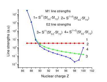
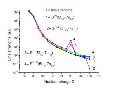
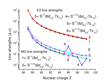
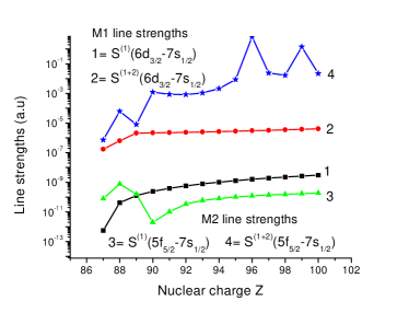
Figure 6: Multipole line strengths ($S$ in a.u) as functions of $Z$ in Fr-like ions.

Table 9: Wavelengths $\lambda$ (Å) and transition rates $A^{(SD)}$ (s^-1) of the electric-quadrupole (E2) and magnetic-multipole (M1 and M3) transitions in Ra II, Ac III, Th IV, and U VI calculated in the SD approximation. Numbers in brackets represent powers of 10.

	Transition		$\lambda$	$A^{\rm(SD)}$	$\lambda$	$A^{\rm(SD)}$
			Ra II, $Z$ = 88		Ac III,$Z$ = 89
E2	$7s_{1/2}$	$6d_{3/2}$	8275.145	1.536[+00]	124844.	1.053[-06]
E2	$7s_{1/2}$	$6d_{5/2}$	7276.373	3.197[+00]	23787.4	3.696[-03]
M3	$7s_{1/2}$	$6d_{5/2}$	7276.373	6.988[-07]	23787.4	7.070[-11]
M1	$7s_{1/2}$	$6d_{3/2}$	8275.145	2.281[-05]	124844.	4.354[-13]
			Th IV, $Z$ = 90		U VI, $Z$ = 90
M1	$5f_{5/2}$	$5f_{7/2}$	23119.6	9.352[-01]	13143.0	5.089[+00]
E2	$5f_{5/2}$	$5f_{7/2}$	23119.6	2.487[-05]	13143.0	1.227[-04]

IV Multipole matrix elements, transition rates, and lifetimes in Fr-like ions

Reduced matrix elements of the electric-quadrupole (E2) and magnetic-multipole (M1, M2, and M3) operators in lowest, second, third, and all orders of perturbation theory are given in Table 8 for Fr-like ions with $Z$ = 88–92. Detailed descriptions of the calculations of the multipole matrix elements in lowest and second orders of perturbation theory were given in Refs. Johnson et al. (1995); Safronova et al. (2001); Hamasha et al. (2004). Third-order and all-order calculations are carried out using the same method as the calculations of E1 matrix elements. In Table 8, we present E2, M1, and M3 matrix elements in the $Z^{(\rm DF)}$, $Z^{(\rm DF+2)}$, $Z^{(\rm DF+2+3)}$, and $Z^{\text{(SD)}}$ approximations for the $6d_{j}-7s_{1/2}$ transitions in Ra II and Ac III and the M1, E2 $5f_{5/2}-5f_{7/2}$ transition in Th IV, Pa V, and U VI. We already mentioned that the ground state in Ra II and Ac III is the $7s_{1/2}$ state with the $6d_{j}$ being the next lowest states; however, the ground state in Th IV, Pa V, and U VI is the $5f_{3/2}$ state with the $5f_{5/2}$ being the next lowest state. The second-order contribution is about 1–3% for all transitions involving the $7s_{1/2}$ states. For the $5f_{5/2}-5f_{7/2}$ transition, the second-order contribution (Coulomb and Breit) is very small (0.1%) for the M1 transition and is rather large (20%) for the E2 transition.

In Fig. 6, we illustrate the $Z$-dependences of the line strengths for the $5f_{5/2}-5f_{7/2}$, $6d{j}-7s_{1/2}$, and $5f_{j}-7ps_{1/2}$ transitions. Two sets of line strengths calculated in first- and second-order approximations are presented for each transition. The values of $S^{(1)}$ and $S^{(1+2)}$ are obtained as $(Z^{(\rm DF)})^{2}$ and $(Z^{(\rm DF+2)})^{2}$, respectively. The difference between $S^{(1)}$ and $S^{(1+2)}$ curves increases with increasing $Z$. For the $5f_{5/2}-5f_{7/2}$ transition, the ratio of the second-order ($S^{(1+2)}$ - $S^{(1)}$) and the first-order ($S^{(1)}$) contributions is equal to 18% and 67% for $Z$ =89 and 95, respectively.

The strong irregularities occur in the curves describing the second-order contributions (see, for example, $S^{(1+2)}(5f_{j}-7s_{1/2}))$ for $Z$ = 96 and $S^{(1+2)}(6d_{3/2}-7s_{1/2}))$ for $Z$ = 95, 99). Those sharp features are explained by accidentally small energy denominators in MBPT expressions for correlation corrections as discussed above.

Wavelengths and transition rates $A^{(SD)}$ for the electric quadrupole (E2) and magnetic-multipole (M1 and M3) transitions in Ra II, Ac III, Th IV, and U VI calculated in the SD approximation are presented in Table 9. The largest contribution to the lifetime of the $6d_{j}$ state in Ra II and Ac III ions comes from the E2 transition, but the largest contribution to the lifetime of the $5f_{7/2}$ state in Th IV  Safronova et al. (2006) and U VI ions comes from the M1 transition. Our SD result for the M1 matrix element in Th IV  Safronova et al. (2006) ion agrees to 0.5% with HFR results obtained by Biémont et al. in Ref. Biémont et al. (2004) since the correlation is small for M1 transition.

Finally, we find that the lifetimes of the $6d_{3/2}$ state is equal to 0.651 s in Ra II and 9.50$\times$10⁵ s in Ac III; the lifetime of the $6d_{3/2}$ state is equal to 0.313 s in Ra II and 271 s in Ac III. The lifetime of the $5f_{7/2}$ state is equal to 1.07 s in Th IV and 0.196 s in U VI.

V Ground state static polarizabilities for Fr-like ions

The static polarizability of Fr-like ions can be calculated as the sum of the polarizability of the ionic core $\alpha_{c}$, a counter term $\alpha_{vc}$ compensating for excitations from the core to the valence shell which violate the Pauli principle, and a valence electron contribution $\alpha_{v}$:

$$\alpha=\alpha_{\mathrm{c}}+\alpha_{\mathrm{v}}+\alpha_{\mathrm{vc}}.$$ (10)

These contributions are given by formulas listed, for example, in Refs. Fowler and Yellin (1970); Safronova and Clark (2004). We calculate $\alpha_{\mathrm{c}}$ in the relativistic RPA approximation (see Ref. Johnson et al. (1983)).

The $7s_{1/2}$ is the ground state in the cases of Fr I, Ra II, and Ac III, and the corresponding polarizability terms are given by

$$\alpha_{\mathrm{v}} = \sum_{n=7}^{N}[I_{v}(np_{1/2})+I_{v}(np_{3/2})],\quad$$ (11)

$$\alpha_{\mathrm{vc}} = \sum_{n=2}^{6}[I_{v}(np_{1/2})+I_{v}(np_{3/2})]\,,$$

where

$$I_{v}(nlj)=\frac{2}{3(2j+1)}\frac{(Z_{v,nlj})^{2}}{E_{nlj}-E_{v}}\,,$$ (12)

and N is the size of B-spline basis set (N = 50 in this calculation). The calculation of the $\alpha_{v}$ is divided into two parts:

$$\alpha_{v}^{\mathrm{main}} = \sum_{n=7}^{k}[I_{v}(np_{1/2})+I_{v}(np_{3/2})];\$$

$$\alpha_{v}^{\mathrm{tail}} = \sum_{n=k+1}^{N}[I_{v}(np_{1/2})+I_{v}(np_{3/2})].$$ (13)

Here, $k$ is equal to 10, 9, and 8 for Fr I, Ra II, and Ac III. The values of $\alpha_{v}^{\mathrm{main}}$ are calculated using SD values of dipole matrix elements $Z_{v,nlj}$ and experimental energies where they are available. We use SD energies when we did not find experimental data. The $\alpha_{v}^{\mathrm{tail}}$. and $\alpha_{\mathrm{c}}$ contributions are small and are calculated in DF approximation.

Our numerical results are given in Table 10. The sum over $n$ in the main polarizability term given by Eq. (V) converges faster for Ac III than for Fr I. The ratios of the second and first terms in sum over $n$ are equal to 1% for Fr I and only 0.1% for Ac III. Therefore, fast convergence allows us to limit the number of $n$ in Eq. (V) to $n$ = 8 in Ac III, since we have no experimental energy values for high $n$ for this ion.

Our SD results for $\alpha_{7s}^{\rm SD}$ given in last line of Table 10 are in good agreement with recommended value (317.7$\pm$2.4) for Fr given by Derevianko et al. in Ref. Derevianko et al. (1999) and recommended value (104.0) for Ra II given recently by Lim and P. Schwerdtfeger in Ref. Lim and Schwerdtfeger (2004). We did not find any data for the $\alpha_{7s}^{\rm SD}$ in Ac III. Our ionic core polarizabilities $\alpha_{c}$ given in Table 10 are in an excellent agreement with recommended values (20.4 in Fr I and 13.7 in Ra II) presented in Refs. Derevianko et al. (1999); Lim and Schwerdtfeger (2004).

The valence polarizability for the $5f_{5/2}$ state, which is the ground state in the case of Fr-like ions with $Z\geq$ 90, is given by  Safronova et al. (2006)

$$\alpha_{{\rm v}}=\sum_{n=n_{0}}^{N}[I_{v}(nd_{3/2})+I_{v}(nd_{5/2})+I_{v}(ng_{7/2})].$$ (14)

Here, $n_{0}$ equal to 6 for the $nd$ states and 5 for the $ng$ states.

We use the same designations as we use for the $7s_{1/2}$ polarizability given by Eqs. (10) - (V). Our results are listed in Table 11. The third-order (DF+2+3) and SD dipole matrix elements (a.u.) are calculated with the 50 splines and cavity radius $R$ = 45 for Th IV. We use use experimental energies Blaise and Wyart to calculate $\alpha_{v}^{\mathrm{main}}$ in Table 11. Both, third-order and all-order results for dipole polarizability of Th IV in the ground state $5f_{5/2}$ are presented in Table 11 (see also Ref. Safronova et al. (2006)). We see from this table that the largest contribution to the $\alpha_{v}^{\mathrm{main}}$ term comes from the $6d$ states ($\alpha_{v}^{\mathrm{main}}(6d)$). The core contribution ($\alpha_{c}$ = 7.750 a₀³) is larger than the main term, limiting the accuracy of our calculations. The $\alpha_{v}^{\mathrm{tail}}$ and $\alpha_{vc}$ terms calculated in the DF approximation contribute only 5% to the final results. No experimental data are available for Th IV polarizability.

The $5f_{5/2}$ ground state polarizabilities for Fr-like ions with $Z$ = 91–100 are given in Table 12. Results are obtained in DF and second-order MBPT approximations. The contribution of the $5g_{7/2}$ state into the $\alpha_{5f_{5/2}}$ polarizability increases with increasing $Z$; 1% for ion with $Z$ = 90 (Th IV), 19% for ion with $Z$ = 92 (U VI), and 30% for ion with $Z$ = 95 (Am IX). The main contributions are smaller than the core contributions. The calculations are conducted only in second-order approximation for these ions, owing to problems with accidentally very small denominators in the corresponding calculations of the properties with involving $5g$ state. We mentioned previously that the core values $\alpha_{\mathrm{c}}(c)$ are calculated in the relativistic RPA approximation following by method described by Johnson et al. in Ref. Johnson et al. (1983). Our $\alpha_{\mathrm{c}}(c)$ results for Ra II – U VI disagree with results presented by Biémont et al. in Ref. Biémont et al. (2004), but agree with Ra II result given in Ref. Lim and Schwerdtfeger (2004).

VI Conclusion

In summary, a systematic relativistic MBPT study of the atomic properties of the $7s_{1/2}$, $7p_{j}$, $6d_{j}$, and $5f_{j}$ states in Fr-like ions with nuclear charges $Z=87-100$ is presented. The energy values are in good agreement with available experimental energy data and provide a theoretical reference database for the line identification. A systematic all-order SD study of the reduced matrix elements and transition rates for eight $7s-7p$, $7p-6d$, and $6d-5f$ electric-dipole transitions is conducted. Multipole matrix elements ($7s_{1/2}\ -6d_{j}$, $7s_{1/2}\ -5f_{j}$, and $5f_{5/2}\ -5f_{7/2}$) are evaluated to obtain the lifetime data for the $6d_{3/2}$ and the $5f_{7/2}$ excited state. The scalar polarizabilities for the $7s_{1/2}$ ground state in Fr I, Ra II, and Ac III and $5f_{5/2}$ ground state in Th IV are calculated using a relativistic third-order and all-order methods. The scalar polarizabilities for Fr-like ions with nuclear charge $Z$ = 90–100 in the $5f_{5/2}$ ground state are calculated using a relativistic second-order MBPT. These calculations provide a theoretical benchmark for comparison with experiment and theory

Table 10: Contribution to the $7s_{1/2}$ static polarizabilities (a.u.) of Fr I, Ra II, and Ac III.

$v=7s_{1/2}$	Fr I	Ra II	Ac III
$\alpha^{{\rm main}}_{v}(7p)$	289.24	93.08	46.74
$\alpha^{{\rm main}}_{v}(8p)$	3.02	0.23	0.06
$\alpha^{{\rm main}}_{v}(9p)$	0.54	0.03
$\alpha^{{\rm main}}_{v}(10p)$	0.19
$\alpha^{{\rm main}}_{v}$	292.99	93.34	46.80
$\alpha^{{\rm tail}}_{v}$	1.20	0.11	0.04
$\alpha_{c}$	20.40	13.79	11.42
$\alpha_{vc}$	-0.95	-0.74	-0.54
$\alpha^{{\rm SD}}_{v}$	313.7	106.5	57.71

Table 11: Contribution to the $5f_{5/2}$ static polarizabilities (a.u.) of Th IV calculated in the third-order - $(a)$ and all-order - $(b)$ approximations.

$v=5f_{5/2}$	$\alpha^{(a)}$	$\alpha^{(b)}$
$\alpha^{{\rm main}}_{v}(6d)$	4.961	6.491
$\alpha^{{\rm main}}_{v}(7d)$	0.009	0.015
$\alpha^{{\rm main}}_{v}(8d)$	0.005	0.007
$\alpha^{{\rm main}}_{v}(5g_{7/2})$	0.063	0.078
$\alpha^{{\rm main}}_{v}(6g_{7/2})$	0.023	0.023
$\alpha^{{\rm main}}_{v}$	5.062	6.612
$\alpha^{{\rm tail}}_{v}$	0.762	0.762
$\alpha_{c}$	7.750	7.750
$\alpha_{vc}$	-0.050	-0.050
$\alpha_{v}$	13.52	15.07

Table 12: Contribution to the $5f_{5/2}$ static polarizabilities (a.u.) in Fr-like ions with $Z$ =91-100 calculated in the DF - $(a)$, second-order - $(b)$, and RPA - $(c)$ approximations.

	$Z$ = 91	$Z$ = 92	$Z$ = 93	$Z$ = 94	$Z$ = 95	$Z$ = 96	$Z$ = 97	$Z$ = 98	$Z$ = 99	$Z$ = 100
$\alpha^{{\rm main}}_{v}(a)$	3.072	1.035	0.548	0.356	0.258	0.199	0.158	0.129	0.106	0.089
$\alpha^{{\rm main}}_{v}(b)$	2.050	0.415	5.935	0.187	0.128	0.083	0.076	0.237	0.120	0.089
$\alpha^{{\rm tail}}_{v}(a)$	0.367	0.206	0.119	0.067	0.036	0.018	0.009	0.005	0.003	0.010
$\alpha_{vc}(a)$	-0.048	-0.044	-0.040	-0.037	-0.033	-0.030	-0.028	-0.025	-0.023	-0.021
$\alpha_{c}(a)$	7.236	5.977	5.023	4.279	3.687	3.207	2.813	2.484	2.207	1.971
$\alpha_{c}(c)$	6.166	5.029	4.182	3.534	3.024	2.615	2.281	2.006	1.776	1.582
$\alpha^{{\rm(DF)}}_{v}$	10.627	7.174	5.649	4.665	3.948	3.394	2.952	2.593	2.293	2.049
$\alpha^{{\rm(DF+2)}}_{v}$	8.535	5.606	10.197	3.751	3.155	2.686	2.338	2.223	1.876	1.660

References

- Biémont et al. (2004) E. Biémont, V. Fivet, and P. Quinet, J. Phys. B 37, 4193 (2004).
- (2) J. Blaise and J. Wyart, Selected constants: energy levels and atomic spectra of actinides, URL=http://www.lac.u-psud.fr/Database/Contents.html.
- Biémont et al. (1998) E. Biémont, P. Quinet, and V. Van Renterghem, J. Phys. B 31, 5301 (1998).
- Simsarian et al. (1999) J. E. Simsarian, W. Z. Zhao, L. A. Orozco, and G. D. Sprouse, Phys. Rev. A 59, 195 (1999).
- Grossman et al. (2000a) J. M. Grossman, R. P. Fliller III, T. E. Mehlstäubler, L. A. Orozco, M. R. Pearson, G. D. Sprouse, and W. Z. Zhao, Phys. Rev. A 62, 52507 (2000a).
- (6) URL = http://physics.nist.gov/PhysRefData/Handbook /Tables/radiumtable6.htm.
- Zhao et al. (1997) W. Z. Zhao, J. E. Simsarian, L. A. Orozco, W. Shi, and G. D. Sprouse, Phys. Rev. Lett. 78, 4169 (1997).
- Simsarian et al. (1998) J. E. Simsarian, L. A. Orozco, G. D. Sprouse, and W. Z. Zhao, Phys. Rev. A 57, 2448 (1998).
- Grossman et al. (2000b) J. M. Grossman, R. P. Fliller III, L. A. Orozco, M. R. Pearson, and G. D. Sprouse, Phys. Rev. A 62, 62502 (2000b).
- Aubin et al. (2003) S. Aubin, E. Gomez, L. A. Orozco, and G. D. Sprouse, Opt. Lett. 28, 2055 (2003).
- Gomez et al. (2005) E. Gomez, L. A. Orozco, A. P. Galvan, and G. D. Sprouse, Phys. Rev. A 71, 62504 (2005).
- Johnson et al. (1996) W. R. Johnson, Z. W. Liu, and J. Sapirstein, At. Data and Nucl. Data Tables 64, 279 (1996).
- Dzuba et al. (1995) V. A. Dzuba, V. V. Flambaum, and O. P. Sushkov, Phys. Rev. A 51, 3454 (1995).
- Dzuba et al. (2001) V. A. Dzuba, V. V. Flambaum, and J. S. M. Ginges, Phys. Rev. A 63, 62101 (2001).
- Safronova et al. (1999) M. S. Safronova, W. R. Johnson, and A. Derevianko, Phys. Rev. A 60, 4476 (1999).
- Safronova and Johnson (2000) M. S. Safronova and W. R. Johnson, Phys. Rev. A 62, 022112 (2000).
- Safronova et al. (2006) U. I. Safronova, W. R. Johnson, and M. S. Safronova, Phys. Rev. A 74, 42511 (2006).
- Savukov et al. (2003) I. M. Savukov, W. R. Johnson, U. I. Safronova, and M. S. Safronova, Phys. Rev. A 67, 042504 (2003).
- Sucher (1980) J. Sucher, Phys. Rev. A 22, 348 (1980).
- Blundell et al. (1989) S. A. Blundell, W. R. Johnson, Z. W. Liu, and J. Sapirstein, Phys. Rev. A 40, 2233 (1989).
- (21) Z. W. Liu, Ph.D. thesis, Notre Dame University, 1989.
- Blundell et al. (1991) S. A. Blundell, W. R. Johnson, and J. Sapirstein, Phys. Rev. A 43, 3407 (1991).
- Safronova et al. (1998) M. S. Safronova, A. Derevianko, and W. R. Johnson, Phys. Rev. A 58, 1016 (1998).
- Safronova and Johnson (2004) U. I. Safronova and W. R. Johnson, Phys. Rev. A 69, 052511 (2004).
- Safronova et al. (1996) M. S. Safronova, W. R. Johnson, and U. I. Safronova, Phys. Rev. A 53, 4036 (1996).
- Safronova et al. (1997) M. S. Safronova, W. R. Johnson, and U. I. Safronova, J. Phys. B 30, 2375 (1997).
- Johnson et al. (1988a) W. R. Johnson, S. A. Blundell, and J. Sapirstein, Phys. Rev. A 37, 307 (1988a).
- Blundell et al. (1987) S. A. Blundell, D. S. Guo, W. R. Johnson, and J. Sapirstein, At. Data and Nucl. Data Tables 37, 103 (1987).
- Johnson et al. (1995) W. R. Johnson, D. R. Plante, and J. Sapirstein, Adv. Atom. Mol. Opt. Phys. 35, 255 (1995).
- Johnson et al. (1988b) W. R. Johnson, S. A. Blundell, and J. Sapirstein, Phys. Rev. A 37, 2764 (1988b).
- Derevianko and Emmons (2002) A. Derevianko and E. D. Emmons, Phys. Rev. A 66, 012503 (2002).
- Savukov and Johnson (2000) I. M. Savukov and W. R. Johnson, Phys. Rev. A 62, 52512 (2000).
- Safronova et al. (2001) U. I. Safronova, W. R. Johnson, D. Kato, and S. Ohtani, Phys. Rev. A 63, 032518 (2001).
- Hamasha et al. (2004) S. M. Hamasha, A. S. Shlyaptseva, and U. I. Safronova, Can. J. Phys. 82, 331 (2004).
- Fowler and Yellin (1970) T. R. Fowler and J. Yellin, Phys. Rev. A 1, 1006 (1970).
- Safronova and Clark (2004) M. S. Safronova and C. W. Clark, Phys. Rev. A 69, 40501R (2004).
- Johnson et al. (1983) W. R. Johnson, D. Kolb, and K. -N. Huang, At. Data and Nucl. Data Tables 28, 333 (1983).
- Derevianko et al. (1999) A. Derevianko, W. R. Johnson, M. S. Safronova, and J. F. Babb, Phys. Rev. Lett. 82, 3589 (1999).
- Lim and Schwerdtfeger (2004) I. S. Lim and P. Schwerdtfeger, Phys. Rev. A 70, 62501 (2004).