The Spitzer c2d Survey of Large, Nearby, Interstellar Clouds. IV. Lupus Observed with MIPS

Abstract

We present maps of 7.78 square degrees of the Lupus molecular cloud complex at 24, 70, and $160\>\mu$m. They were made with the Spitzer Space Telescope’s Multiband Imaging Photometer for Spitzer (MIPS) instrument as part of the Spitzer Legacy Program, “From Molecular Cores to Planet-Forming Disks” (c2d). The maps cover three separate regions in Lupus, denoted I, III, and IV. We discuss the c2d pipeline and how our data processing differs from it. We compare source counts in the three regions with two other data sets and predicted star counts from the Wainscoat model. This comparison shows the contribution from background galaxies in Lupus I. We also create two color magnitude diagrams using the 2MASS and MIPS data. From these results, we can identify background galaxies and distinguish them from probable young stellar objects. The sources in our catalogs are classified based on their spectral energy distribution (SED) from 2MASS and Spitzer wavelengths to create a sample of young stellar object candidates. From 2MASS data, we create extinction maps for each region and note a strong corresponence between the extinction and the $160\>\mu$m emission. The masses we derived in each Lupus cloud from our extinction maps are compared to masses estimated from ¹³CO and C¹⁸O and found to be similar to our extinction masses in some regions, but significantly different in others. Finally, based on our color-magnitude diagrams, we selected 12 of our reddest candidate young stellar objects for individual discussion. Five of the 12 appear to be newly-discovered YSOs.

1. Introduction

The Spitzer Legacy Science Program, “From Molecular Cores to Planet-Forming Disks” (c2d) (Evans et al., 2003), mapped five nearby molecular clouds using the Spitzer Space Telescope (hereafter Spitzer) (Werner et al., 2004). This paper, fourth in a series of papers, presents the basic results from the Multiband Imaging Photometer for Spitzer (MIPS) (Rieke et al., 2004) for the Lupus Molecular cloud complex.

The Lupus molecular cloud complex covers a broad range of Galactic longitude and latitude and consists of a number of distinct regions (Krautter, 1991). The cloud is located near the Scorpius-Centaurus OB association. The large spatial extent of Lupus on the sky ($\sim 20^{\circ}$) means that different regions in the cloud may be at different distances. Hipparcos measurements to nearby OB star sub-groups within Scorpius-Centaurus give average distances of $\sim 140$ pc (de Zeeuw et al., 1999). This distance is in agreement with various reddening studies (e.g. Franco, 1990). Distance estimates derived from Hipparcos parallaxes to individual stars within the Lupus clouds can vary by more than a factor of two, suggesting that depth effects are important in the Lupus cloud complex (Wichmann et al., 1998; Bertout et al., 1999). For this paper we are adopting distances of $150\pm 20$ pc for Lupus I and IV and $200\pm 20$ pc for Lupus III. See Comerón (2007, and references therein) for a full discussion on the difficulties in obtaining accurate distance measurements to Lupus.

Compared to other c2d clouds, Lupus is a relatively quiescent star-forming cloud. Comerón (2007) has compiled a table of all the known classical T-Tauri Stars (cTTSs) in different Lupus regions. Within the area we observed with both the InfraRed Array Camera (IRAC) (Fazio et al., 2004) and MIPS instruments, there are 5 CTTSs in Lupus I, 32 in Lupus III, and 3 in Lupus IV. In addition to the known CTTSs, Comerón (2007) lists 19 new suspected very low-mass members of Lupus III with likely H$\alpha$ emission (López Martí et al., 2005), and 4 recently discovered M-type members in Lupus III (Comerón et al., 2003). Over 100 weak-line T-Tauri stars (WTTSs) were discovered with ROSAT (Krautter et al., 1997), extending over a much larger region than the dark clouds. Based on velocity dispersions and positions, Wichmann et al. (1997) speculated that these WTTSs may have formed earlier and since moved away from the dark clouds.

We summarize our observations in § 2 and our data processing pipeline in § 3. A full description of the data processing used on all c2d data is available in our delivery documentation (Evans et al., 2007). For this paper, we made ‘MIPS high-reliability’ cuts to the c2d catalogs, as described in § 4. Our results are summarized in § 5.

Our goals in this paper are to present the c2d Lupus MIPS data and identify the likely young stellar members of the Lupus cloud. We plot the differential source counts at $24\>\mu$m for our cloud regions and compare these to model predictions and observed off-cloud fields (§ 5.1). We use the 2MASS and MIPS data to create two color-magnitude diagrams (§ 5.2) which are useful in distinguishing background galaxies from young stellar objects. We create a sample of ‘Young Stellar Object (YSO) candidates’ based on each source’s spectral energy distribution in the 2MASS and Spitzer wavebands and discuss the significance of our sample in relation to previously know YSOs (§ 5.3). Because YSOs are typically found in the densest regions, we create extinction maps from 2MASS, estimate the mass in each cloud region, and compare the extinction maps to the $160\>\mu$m emission (§ 5.4). Finally, from our ‘YSO candidate’ sample and the color-magnitude diagrams, we select 12 likely young stellar objects. These sources are discussed individually in § 5.5.

2. Observations

Table 1 Summary of Observations

Region	AOR Number	Date Observed	Program ID
		YYYY-MM-DD
Lupus I	0005723648	2004-08-24	175
	0005722880	2004-08-23	175
	0005723904	2004-08-24	175
	0005723136	2004-08-24	175
	0005724160	2004-08-24	175
	0005722624	2004-08-23	175
	0005722368	2004-08-23	175
	0005723392	2004-08-24	175
Lupus III	0005727232	2004-08-24	175
	0005728000	2004-08-24	175
	0005727488	2004-08-24	175
	0005727744	2004-08-24	175
	0005728256	2004-08-24	175
	0005728512	2004-08-24	175
Lupus IV	0005730304	2004-08-24	175
	0005730560	2004-08-24	175
Lupus OC1	0005734400	2004-08-24	175
	0005734656	2004-08-24	175
Lupus OC2	0005734912	2004-08-24	175
	0005735168	2004-08-24	175

Our observations of Lupus cover three separate on-cloud regions and two off-cloud regions. We designate the on-cloud regions as I, III, and IV following the convention from Cambrésy (1999). The total mapped area on-cloud in two epochs is approximately 7.78 square degrees. In addition to the on-cloud maps, we observed two small off-cloud regions for reference, designated off-cloud 1 (OC1) and off-cloud 2 (OC2). In Figure 1, the observed $24\>\mu$m areas for each region are overlaid on the $25\>\mu$m IRAS map. The observed areas at $70$ and $160\>\mu$m are very similar in size, shape, and position to those at $24\>\mu$m. Table 1 lists the Astronomical Observing Request (AOR) numbers, dates observed, and Spitzer program ID for all our observations.

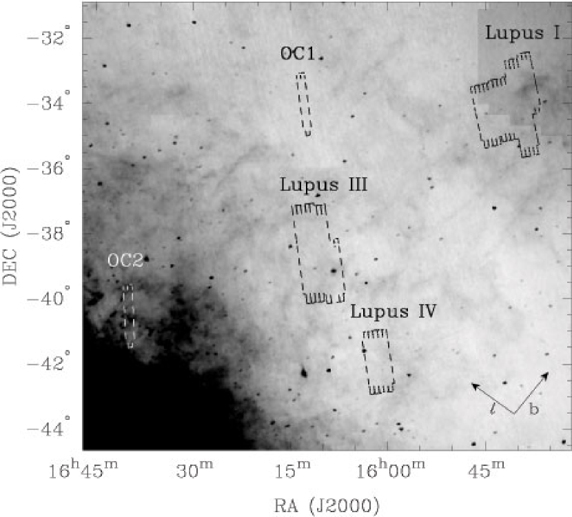
Figure 1.— Map showing the observed regions in the Lupus cloud. These regions are designated: Lupus I, Lupus III, Lupus IV, and two off-cloud regions (OC1 and OC2). The outlines show the mapped areas at $24\>\mu$m; the 70 and $160\>\mu$m coverage maps are very similar. The grayscale image is the IRAS 25 $\mu$m emission. The saturated region at the lower left is the Galactic plane. The directions of increasing Galactic longitude and latitude are denoted by arrows in the lower right corner.

We used the optical extinction maps of Cambrésy (1999) to choose the areas mapped. Lupus I covers areas with extinctions $A_{V}\geq 3$, while Lupus III and IV map extinctions $A_{V}\geq 2$. The two off-cloud regions had $A_{V}<0.5$ in the optical extinction maps. Lupus II was not observed because there was very little area in the extinction map with $A_{V}\geq 2$. Due to time constraints, we did not observe Lupus V or VI. It is worth noting, however, that there is no obvious evidence of recent or current star formation in these regions (Comerón, 2007). Information on the observed regions, including mapped area, distance, and approximate Galactic coordinates are listed in Table 2.

Table 2 Basic Information on the Observed Regions

Region	$l$	$b$	dist.	size	median $A_{V}$	Mass ($A_{V}\geq 3$)
	(deg.)	(deg.)	(pc)	(deg2)	(mag)	($M_{\odot}$)
Lupus I	338	17	150	3.82	1.8	440
Lupus III	340	9	200	2.88	2.4	690
Lupus IV	336	8	150	1.08	2.2	250
Lupus OC1	344	12	$\cdots$	0.31	0.7	$\cdots$
Lupus OC2	343	4	$\cdots$	0.31	2.1	$\cdots$

Note. — The approximate Galactic latitude and longitude, distance, mapped area, median $A_{V}$, and mass are listed for the three on-cloud regions and the two off-cloud regions. The masses are derived in § 5.4. See Comerón (2007) for a discussion of the adopted distances to each region. The map size listed is the size of the $24\>\mu$m map covered in both epochs. The regions observed at 70 and $160\>\mu$m are of similar size.

All data were taken in MIPS fast-scan mode with a $240^{\prime\prime}$ offset between scan legs. A second epoch of observation was taken later to help identify asteroids. The time between the two epochs of observation ranged from 3.5 hours in Lupus I to almost 7 hours in Lupus III. The second epoch is offset, compared to the first, by $125^{\prime\prime}$ in the cross-scan direction. Furthermore, to fill in gaps at $160\>\mu$m, the second epoch is offset by $80^{\prime\prime}$ along the scan direction. Only half of the $70\>\mu$m array returns usable data. To minimize this effect, the AORs were planned such that the second epoch would fill in the holes in the $70\>\mu$m maps. The net result is that the $24$ and $70\>\mu$m maps have approximately the same coverage, but the total integration time per pixel at $70\>\mu$m is 15 seconds, compared to 30 seconds at $24\>\mu$m. The integration time per pixel is roughly 3 seconds at $160\>\mu$m.

3. Data Reduction

The c2d team has made regular deliveries of mosaics and bandmerged catalogs to the Spitzer Science Center (SSC) for c2d regions. The delivery documentation and data used in this paper can be found on the SSC website under delivery 4, the final data delivery of the c2d team. Detailed discussion of the data reduction method applied to all c2d products can be found in the delivery documentation (Evans et al., 2007). In this paper we will give only a brief outline of the standard processing procedure. We will discuss the steps of this procedure in the order they are performed. For this paper, as in delivery 4, we processed all the data with the S13 SSC pipeline.

We made two changes to the standard c2d processing procedure. First, for display purposes only, we made several cosmetic improvements to the $70\>\mu$m and $160\>\mu$m images. These enhanced images were created from the older S11 SSC products. The specific improvements will be discussed in § 3.1. Source extraction and photometry at these wavelengths is performed with the standard SSC filtered and unfiltered data products using the c2d pipeline. Our second change compared to the standard c2d processing procedure is that at $160\>\mu$m we bandmerged the c2d extractions with the c2d catalog.

This paper is one of a series of papers to present the c2d observations of clouds in a uniform manner. The first paper in this series presented MIPS results for Chamaeleon II (Young et al., 2005). That paper used an earlier version of the SSC pipeline, S9.5. Other papers that present MIPS results from the c2d clouds use the S13 products as we have here (Rebull et al., 2007; Harvey et al., 2007; Padgett et al., 2007). Despite some differences in data processing, many of the figures are standardized to facilitate comparisons between c2d clouds.

3.1. Image Processing

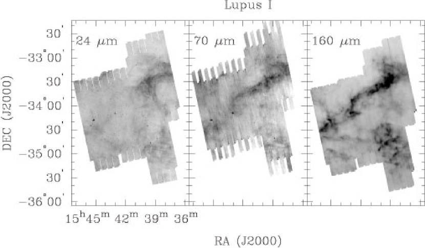
Figure 2.— The 24, 70, and $160\>\mu$m images of Lupus I. We have applied several cosmetic corrections to the 70 and $160\>\mu$m images as described in § 3.1.

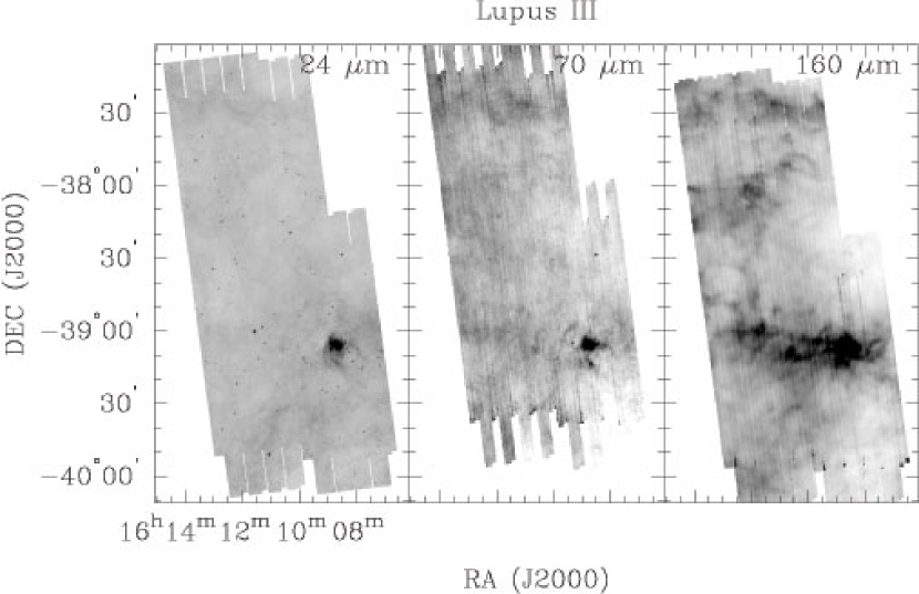
Figure 3.— The 24, 70, and $160\>\mu$m images of Lupus III. We have applied several cosmetic corrections to the 70 and $160\>\mu$m images as described in § 3.1.

Starting from the Basic Calibrated Datasets (BCDs), the c2d team further processed the $24\>\mu$m images to remove some instrumental effects. We corrected a “jailbar” response pattern that is caused by bright sources or cosmic rays by applying an additive correction to the low readouts to bring them up to the same level as the high readouts. Additionally, the first four frames in a map were scaled to the median of following frames, and each AOR was self-flattened to eliminate a small instrumental brightness gradient along the column direction and other residual image artifacts.

The SSC provided two sets of BCD products for the 70 and 160 $\mu$m data, unfiltered (normal processing) and filtered (a time median filter is applied). We have further processed the SSC’s unfiltered $70\>\mu$m data to improve the visual appearance of the mosaic image. The first correction we made was to subtract out the latent signal from stimulator (stim) flashes. The signal after the latent had faded was used as a reference to subtract out the stim flash latents. Further, the SSC unfiltered products contained a striped pattern roughly along the column direction, which was caused by response variations. We self-flattened the data with a median obtained from the frames in each scan leg to reduce this effect.

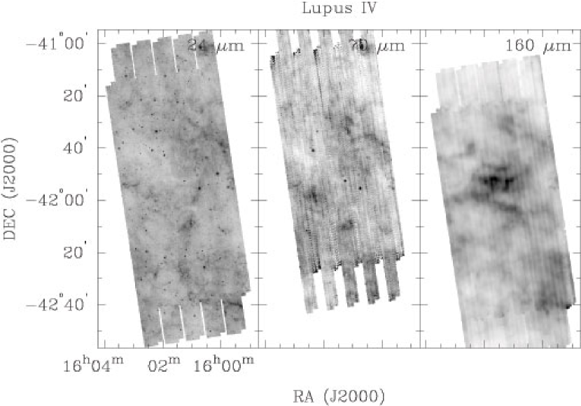
Figure 4.— The 24, 70, and $160\>\mu$m images of Lupus IV. We have applied several cosmetic corrections to the 70 and $160\>\mu$m images as described in § 3.1.

We have made visually enhanced $160\>\mu$m mosaics by excluding the stim flash BCDs and the following frames that contained a latent signal. The mosaic was then created with $8\arcsec$ pixels, half the natural pixel scale (twice the resolution). Lastly, the image was smoothed with a median filter, where each pixel in the image was replaced by the median of the values within a $7\times 7$ pixel box. Pixels with a value of NaN were treated as missing data during this filtering.

Figures 2 - 4 show the 24,70, and 160 $\mu$m images in separate panels for regions I, III, and IV, respectively. We have also combined these three wavelengths to make a color image where red represents the $160\>\mu$m, green the $70\>\mu$m, and blue the $24\>\mu$m emission. The color images for Lupus I, III, and IV are shown in Figures 5 - 7.

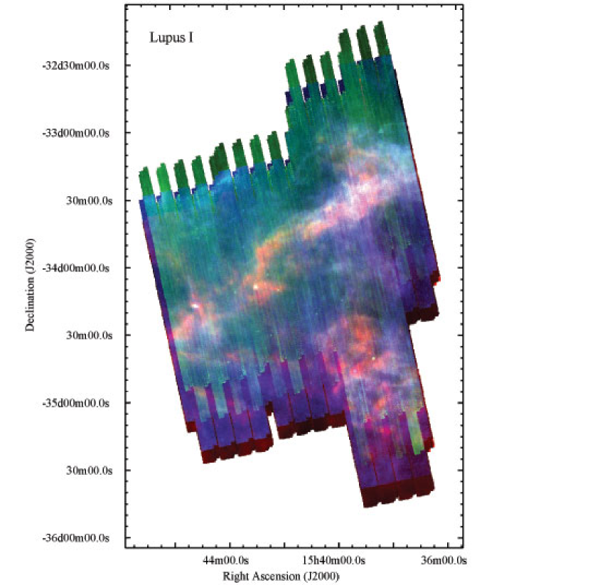
Figure 5.— A pseudo-color image for Lupus I showing the 24, 70, and $160\>\mu$m emission in the blue, green, and red channels, respectively. We have applied several cosmetic corrections to the 70 and $160\>\mu$m images as described in § 3.1.

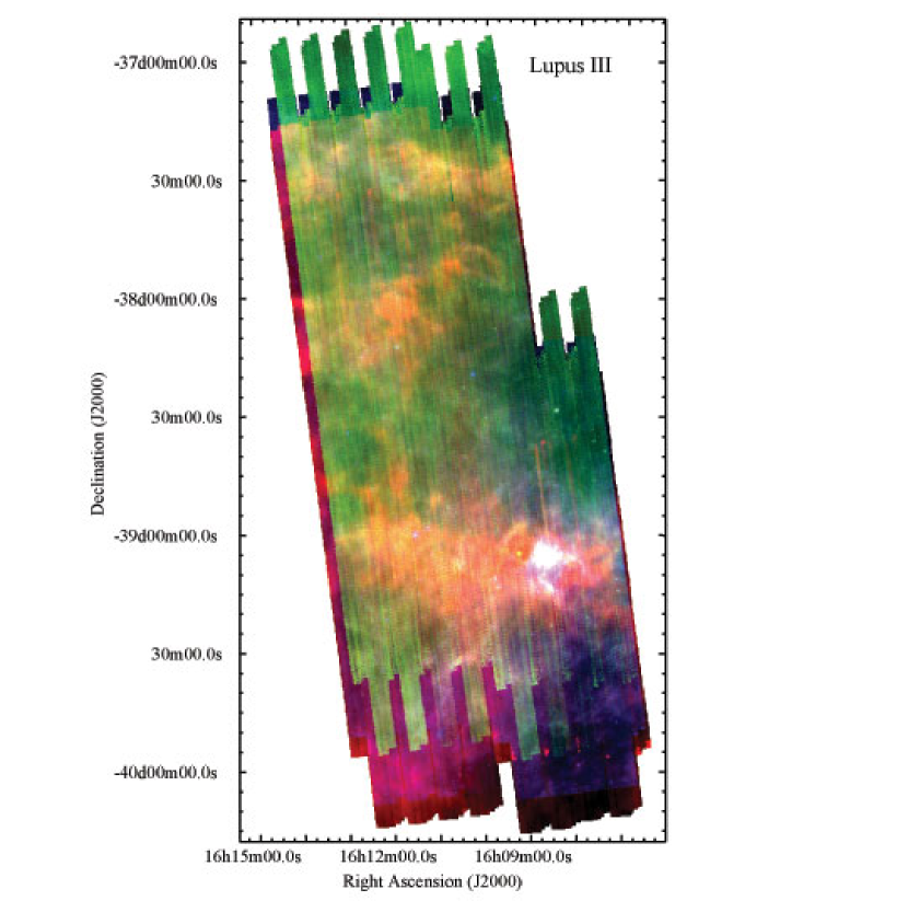
Figure 6.— A pseudo-color image for Lupus III showing the 24, 70, and $160\>\mu$m emission in the blue, green, and red channels, respectively. We have applied several cosmetic corrections to the 70 and $160\>\mu$m images as described in § 3.1.

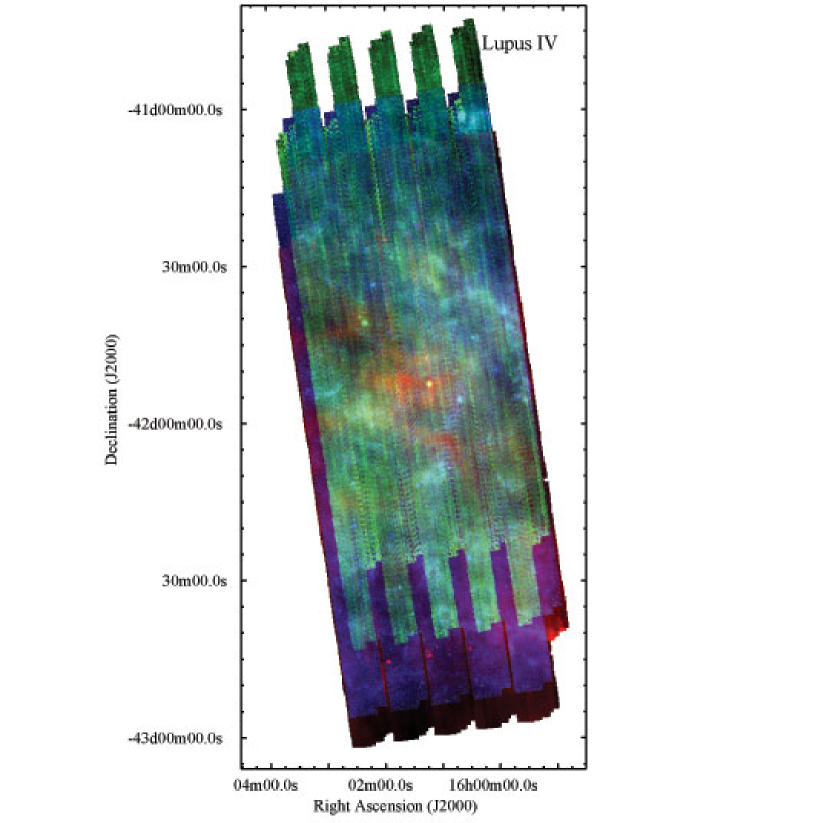
Figure 7.— A pseudo-color image for Lupus IV showing the 24, 70, and $160\>\mu$m emission in the blue, green, and red channels, respectively. We have applied several cosmetic corrections to the 70 and $160\>\mu$m images as described in § 3.1.

3.2. Mosaicking and Source Extraction

We created mosaic images at $24\>\mu$m using the SSC’s MOPEX program (Makovoz & Marleau, 2005) with the outlier rejection and position refinement modules. Three sets of mosaics were created, one for each epoch separately and one combined epochs mosaic. We used the improved BCDs described in § 3.1 for these mosaics. Outlier rejection excluded bad pixels caused by cosmic rays or image artifacts. The initial identification of point sources was performed on each mosaic using a modified version of the DOPHOT program (Schechter et al., 1993). This program works by fitting point spread functions, so as sources were found, they were subtracted from the image. This procedure was iterated until a user defined flux limit was reached. We calculated the final position and photometry for each source using all BCD images that contributed to that source.

The $24\>\mu$m source fluxes were calibrated by computing the ratio between the aperture flux and model point spread function (PSF) flux for all sources with a reliable aperture flux that could be fitted by the point source profile. We assumed the average aperture to PSF flux ratio held for all sources, and a multiplicative correction was applied.

The $70\>\mu$m point source extractions were performed on mosaic images made using MOPEX on the SSC’s filtered and unfiltered BCDs, not the enhanced mosaics described in § 3.1. We used APEX, the SSC’s point source extraction software, on both the filtered and unfiltered mosaic images to obtain point sources. We used the point response function (PRF) photometry from the filtered mosaic except for sources brighter than $\sim 2$ Jy, when the SSC’s filtering over corrects in the wings of the PRF. In such cases, we substituted PRF photometry from the unfiltered mosaic.

At $160\>\mu$m we performed source detection and photometry using the MOPEX package on the SSC’s unfiltered BCD mosaics. Again, we did not use the enhanced mosaics created in § 3.1. Fluxes were determined by point-source fitting. Sources that were close multiples, extended, or had S/N $<5$ are not listed here. For saturated sources, we assumed the object was a point source and fit the wings of the PSF to find the flux. Sources which were detected but deemed unreliable by visual inspection were dropped. Because of this culling, the 160 $\mu$m source list is believed to be reliable but not complete, and no completeness limit is given.

The c2d team estimates the absolute flux uncertainty is 15% at $24\>\mu$m and $20$% for $70$ and $160\>\mu$m. We estimate the relative flux uncertainty to be approximately $5$% plus the statistical uncertainty for each source.

3.3. Bandmerging

The final stage of data processing prior to science analysis of c2d images involves the creation of bandmerged catalogs. Again, refer to the c2d delivery document (Evans et al., 2007) for details. Even though this paper focuses on MIPS results, IRAC bandmerging is also described since these wavelengths are used for source classification (§ 3.4) and when discussing individual sources (§ 5.5).

3.3.1 IRAC - MIPS 24 Bandmerging

For each band, the three source extraction lists (epoch1, epoch2, and combined epochs) were checked for “self-matches” within an epoch; two sources extracted within one epoch, but with positional matches of $\leq\>2\farcs 0$ were considered to be the same source. The fluxes of the detections were summed, and the position of the source was calculated as the weighted mean. We then merged the three lists together to cross-identify sources with positional matches of $2\farcs 0$ or less. We visually inspected the epoch-merged source lists for each band to remove diffraction spikes, column pull-down, latent images, and other image artifacts that were misidentified as sources.

The epoch-merged source lists for each band were then merged as follows: First, we merged the four IRAC bands together, one-at-a-time. We started by merging IRAC1 ($3.6\>\mu$m) and IRAC2 ($4.5\>\mu$m), then merged this product with IRAC3 ($5.8\>\mu$m), and finally combined with IRAC4 ($8\>\mu$m). At each step, we combined detections at two wavelengths into a single source if the difference in central position was $\leq\>2\farcs 0$. Then, this bandmerged IRAC catalog was merged with the $24\>\mu$m MIPS1 band using a larger distance, $4\farcs 0$. The larger distance was used because of the larger PSF at $24\>\mu$m compared to IRAC. Lastly, the IRAC+MIPS1 catalog was compared with the 2MASS catalog using a position matching criterion of $2\farcs 0$.

In all steps of bandmerging, IRAC, MIPS1, and 2MASS, we merged together the closest position match between 2 wavelengths. Any other detections within the specified radius were preserved in the final catalog, but not merged.

3.3.2 MIPS $70\>\mu$m and $160\>\mu$m Bandmerging

Even though we have two epochs of observation at $70\>\mu$m, they do not have much overlap between them. Thus, we only performed source extractions on the combined epochs dataset. First, we performed a ‘self-merging’ on the combined epochs dataset using a matching radius of $4\farcs 0$. Secondly, each $70\>\mu$m point source detection was matched to all shorter wavelength catalog sources within a $8\farcs 0$ radius. We then visually inspected each merged $70\>\mu$m detection to determine the ‘best’ source match between shorter wavelengths ($1.25-24\>\mu$m) and $70\>\mu$m. This ‘best’ source match was the one with the most consistent Spectral Energy Distribution (SED) across all detected wavelengths. In a few cases where it was not clear which SED was ‘better’, we chose the closer match.

Shorter wavelength sources that were within $8\farcs 0$ of a $70\>\mu$m detection but not matched with the $70\>\mu$m, were assigned a special flag to denote their status. Thus, in our final catalog, a $70\>\mu$m detection is listed once; we did not try to split up the flux to different shorter wavelength sources.

There are so few $160\>\mu$m point sources that they were bandmerged individually by eye for those selected sources described in § 5.5.

3.4. Source Classification

After bandmerging, we classified sources based on their SEDs at wavelengths from $1.25-24\>\mu$m. Even though this paper concentrates on the MIPS results for Lupus, we utilized the IRAC and 2MASS wavelengths for source classification. The two most important categories for the work discussed here are ‘star’ and ‘Young Stellar Object candidate (YSOc)’. Objects classified as ‘star’ have measurements in 3 or more bands and the SED can be fitted by a reddened stellar photosphere (including the 2MASS data if available). In addition, if a source had an SED that could be fitted by a reddened photosphere except in one band, we also classified it as ‘star’, assuming that it has a prominent spectral line feature that changed the shape of the SED. A future paper will explore our source classification method in depth (Lai et al., in prep.).

It is important to include the effect of dust extinction when identifying stars, because star light is often dimmed by significant dust in the molecular clouds we observed. The observed flux of a reddened star, $F_{obs}(\lambda)$, can be described with the following equation:

$$\log(F_{obs}(\lambda)/F_{model}(\lambda))=\log(K)-0.4\times C_{ext}(\lambda)\times A_{V}$$ (1)

where $F_{model}(\lambda)$ is the stellar photosphere model, $K$ is the scaling factor of the model for a particular star, and $C_{ext}(\lambda)\equiv A_{\lambda}/A_{V}$ is the ratio of extinction at wavelength $\lambda$ to visual extinction from the dust extinction law. $K$ and $A_{V}$ can be derived from the linear fit of this equation by adopting stellar photosphere and dust extinction models. The stellar photosphere models for $K_{s}$–MIPS1 bands are based on the Kurucz-Lejeune models and come from the SSC’s “Star-Pet” tool. For the 2MASS bands, we translated the observed $J-H$ and $H-K$ colors of stars (Koornneef, 1983) to fluxes relative to $K$ band and ignored the difference between $K$ and $K_{s}$ bands. We used a dust extinction model with a ratio of selective-to-total extinction ($R_{V}$) of 5.5 (Weingartner & Draine, 2001, their case “B”). This model is a good match to the Indebetouw et al. (2005) extinction law study using the Spitzer IRAC bands.

YSO candidates are traditionally selected from sources with excess flux at near- to far-infrared wavelengths compared to the stellar photosphere. Unfortunately, most (if not all) background galaxies fit the same description. In order to create a sample strongly enriched in YSOs, we have used several statistical criteria derived from the SWIRE data of ELAIS N1 (Surace et al., 2004) to separate ‘YSO candidates’ from other objects with infrared excesses. The Spitzer Wide-area InfraRed Extragalactic (SWIRE) survey imaged six separate fields selected to be away from the Galactic plane and free from interstellar dust. The ELAIS N1 region, located towards the Galactic North Pole, presumably contains almost nothing other than non-YSO stars and background galaxies making it useful for understanding the distribution of infrared excess non-YSO sources.

We used both IRAC and MIPS data together to identify ‘YSO candidates’. The criteria we used were empirically derived from SWIRE and the Serpens molecular cloud. Detailed discussion can be found in the delivery documentation and Harvey et al. (2007). In brief, we constructed “probability” functions from three color-magnitude diagrams: [4.5] vs. [4.5] - [8.0], [24] vs. [4.5] - [8.0], and [24] vs. [8.0] - [24]. Based on where a source lies in each color-magnitude diagram, it is assigned a probability of being a galaxy. The final probability is then the product of the three individual probabilities, and if it is less than a set value, the source is classified as a ‘YSO candidate’.

4. Final Catalogs

All catalogs discussed in the paper are available on the SSC website under the delivery 4 products. Separate catalogs of all ‘YSO candidates’ in Lupus are also available from the same location.

4.1. Main Lupus Catalogs

In addition to the visual inspection performed during bandmerging, we made two further cuts on the data to obtain a high reliability catalog for each cloud region. First, we required all $24\>\mu$m detections to be at least $3\sigma$ in the combined epochs (quality of detection “A”, “B”, or “C”). Asteroid contamination is also a problem in Lupus since the cloud is located near the plane of the ecliptic (latitude -14 to -21 degrees). To eliminate asteroids, we imposed the requirement that a source be detected at $24\>\mu$m in both of the single epochs of observation and in the combined epochs data. Because our two epochs of observation were separated in time by $3-7$ hours, the asteroids would have moved sufficiently that they would not be detected in both epochs at the same position. A broader statistical analysis of field asteroids in Spitzer Legacy datasets will be presented in Stapelfeldt et al. (in prep.). Our catalogs contain 1790 sources in Lupus I, 1950 in Lupus III, and 770 in Lupus IV. In this paper, we only use these ‘MIPS high-reliability’ catalogs.

4.2. c2d Processed $24\>\mu$m SWIRE Catalogs

We have compared our results to the SWIRE data for ELAIS N1 (Surace et al., 2004). Because this region maps the Galactic north pole, the sources should be almost entirely non-YSO stars or background galaxies. Thus, this data set is valuable in distinguishing YSOs from galaxies. We processed a portion of the SWIRE BCDs for ELAIS N1 with the c2d data pipeline and created our own c2d-processed SWIRE catalog. This catalog has only one epoch of observation for MIPS. However, ELAIS N1 is located at $\sim+70$ ecliptic latitude so asteroid contamination is not a concern.

The SWIRE data is more sensitive at all wavelengths than our c2d observations. To make comparisons between SWIRE and c2d, we have created resampled SWIRE catalogs that simulate the sensitivity of our c2d observations. This resampling involves: (1) extincting the SWIRE sources consistent with positioning these sources behind each Lupus region; (2) randomly selecting faint SWIRE detections to flag as non-detections in the resampled catalog in order to match sensitivity with c2d; (3) replacing the photometric errors with ones more characteristic of c2d observations; and (4) re-classifying the sources in the resampled catalog as described in § 3.4.

After resampling, we have three c2d-processed SWIRE catalogs, one each for Lupus I, III, and IV. To create ‘MIPS high-reliability’ catalogs similar to above, we have also required a detection at $24\>\mu$m to be at least $3\sigma$ (quality of detection “A”,“B”, or “C”). Our catalogs contain 1588 sources (Lupus I), 1646 (Lupus III), and 2061 (Lupus IV). Each one covers 5.3 deg². We will use these resampled, ‘MIPS high-reliability’ c2d-processed SWIRE catalogs in this paper.

4.3. Lupus Off-Cloud regions

We observed two off-cloud regions, called OC1 and OC2. For the analysis in this paper, we will only be using OC1. OC1 is located at a higher Galactic latitude compared to OC2. The Galactic latitude for OC1 is closer to the latitude of the three cloud regions. Because of this, the source counts and source classifications in OC1 provide the best comparison with the on-cloud regions. We made the same ‘MIPS high-reliability’ cuts to the data as used for the on-cloud catalogs. Our OC1 catalog contains 157 sources.

5. Results

5.1. $24\>\mu$m Source Counts

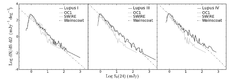
Figure 8.— Differential source counts at 24 microns for the three Lupus regions. Four different curves are displayed: The on-cloud source counts (black), Lupus off-cloud 1 (dotted), resampled SWIRE (gray), and 25 micron Wainscoat galaxy model counts (dot-dashed) (Wainscoat et al., 1992). The Wainscoat model in each panel was computed for the Galactic latitude, longitude, distance, and average $A_{V}$ of the specified Lupus region using the values listed in table 2.

Figure 8 shows the $24\>\mu$m differential source counts per square degree for Lupus I, III, and IV. For comparison, we also show the source counts per square degree for Lupus OC1, our c2d-processed SWIRE catalogs, and the predicted values from the Wainscoat model at 25 microns (Wainscoat et al., 1992). The Wainscoat model counts were produced separately for Lupus I, III, and IV using the Galactic longitude, latitude, distance, and median $A_{V}$ present within the each region. These parameters are listed in Table 2. We did not apply a correction for the difference between the IRAS $25\>\mu$m counts output from the Wainscoat model and our plotted $24\>\mu$m differential source counts. The source counts for every curve were binned with a bin width of 0.1 mag., the same bin width produced by the Wainscoat model.

In all areas, both on- and off-cloud, the counts peak around 1 mJy and drop off dramatically below this flux due to the completeness limit. Brighter than $\sim 10$ mJy, there are too few $24\>\mu$m sources in OC1 to make a reliable histogram. Therefore we have not plotted this curve past $10$ mJy. For fainter fluxes, the source counts for OC1 are consistent with all three Lupus cloud regions.

The predicted source counts from the Wainscoat model agree well with the actual on-cloud source counts for Lupus I, III, and IV. The only significant difference from the model is below $\sim 3$ mJy in Lupus I. Here, the on-cloud counts are higher than those predicted by the Wainscoat model, but are consistent with the resampled SWIRE counts, suggesting that these sources may be extragalactic. For Lupus III and IV, the on-cloud counts are slightly higher than the SWIRE counts at all fluxes. Because Lupus III and IV are consistent with the Wainscoat model, the higher counts are likely due to Galactic sources. This explanation is consistent with the relative Galactic latitudes of each cloud. Lupus I, at $+17$, should have a higher fraction of extragalactic sources compared to Lupus III and IV which are at lower latitudes, and thus should have a higher fraction of Galactic sources.

5.2. MIPS Color-Magnitude Diagrams

Table 3 Individual YSO Candidates

Index	Region	Source Name	RA (J2000)	DEC (J2000)	SSC ID	Class
1	I	IRAS 15356-3430	15:38:48.4	-34:40:38.2	SSTc2d J153848.4-344038.2	I
2	I	IRAS 15398-3359	15:43:02.3	-34:09:07.5	SSTc2d J154302.3-340907.5	I
3	I	2MASS 15450634	15:45:06.3	-34:17:38.1	SSTc2d J154506.3-341738.1	Flat
4	I	2MASS 15450887	15:45:08.9	-34:17:33.7	SSTc2d J154508.9-341733.7	II
5	III	2MASS 16070854	16:07:08.6	-39:14:07.7	SSTc2d J160708.6-391407.7	Flat
6	III	Sz 102	16:08:29.7	-39:03:11.0	SSTc2d J160829.7-390311.0	I
7	III	IRAS 16051-3820	16:08:30.7	-38:28:26.8	SSTc2d J160830.7-382826.8	II
8	III	IRAS 16059-3857	16:09:18.1	-39:04:53.4	SSTc2d J160918.1-390453.4	I
9	IV	2MASS 16011549	16:01:15.6	-41:52:35.3	SSTc2d J160115.6-415235.3	Flat
10	IV	IRAS 15587-4125	16:02:13.1	-41:33:36.3	SSTc2d J160213.1-413336.3	I
11	IV	IRAS 15589-4132	16:02:21.6	-41:40:53.7	SSTc2d J160221.6-414053.7	I
12	IV	2MASS 16023443	16:02:34.5	-42:11:29.7	SSTc2d J160234.5-411129.7	Flat

Note. — Names, positions, and classifications of individual YSO candidates discussed in § 5.5. The index numbers identify the sources in the figures. Classifications are based on the criteria of Greene et al. (1994).

Table 4 Fluxes for Selected YSO Candidates

	2MASS				IRAC					MIPS
Index	$J$	$H$	$K_{s}$		$3.6\>\mu$m	$4.5\>\mu$m	$5.8\>\mu$m	$8.0\>\mu$m		$24\>\mu$m	$70\>\mu$m	$160\>\mu$m
	(mJy)	(mJy)	(mJy)		(mJy)	(mJy)	(mJy)	(mJy)		(mJy)	(mJy)	(mJy)
1	2.15	3.84	6.60		3.95	2.76	9.58	42.7		114	2920	4230
2	$\cdots$	$\cdots$	$\cdots$		1.97	23.2	42.6	127		961	15300	57200
3	0.955	4.01	9.61		14.1	15.4	16.2	19.1		69.9	204	$\cdots$
4	21.1	56.7	87.4		101	104	100.	94.3		137	702	$\cdots$
5	1.30	5.73	15.8		32.9	48.3	60.6	89.3		196	189	$\cdots$
6	2.39	3.54	6.19		14.4	24.1	34.0	67.0		347	257	$\cdots$
7	410.	452.	342.		$\cdots$	$\cdots$	$\cdots$	$\cdots$		473	2200	2210
8	$\cdots$	$\cdots$	$\cdots$		0.255	1.00	0.985	0.549		32.4	2610	8710
9	0.424	1.67	4.83		8.36	9.92	8.98	7.70		75.9	1220	5390
10	2.94	2.12	1.97		$\cdots$	2.11	$\cdots$	3.80		533	276	$\cdots$
11	1.63	3.36	4.66		5.10	4.87	12.6	42.1		144	1030	2340
12	4.39	7.45	14.0		31.1	$\cdots$	41.5	$\cdots$		118	269	$\cdots$

Note. — The 2MASS and Spitzer fluxes for the twelve selected sources in Table 3. The SEDs for these sources are plotted in Figure 17. The statistical uncertainty in these fluxes is less than the absolute photometric error. As discussed in the delivery documentation (Evans et al., 2007) and in § 3.2, the absolute photometric error is estimated to be $15\%$ for $3.6-24\>\mu$m and $20\%$ at 70 and $160\>\mu$m.

We plotted color-magnitude diagrams for each Lupus region in Figures 9 and 10. In each figure, the resampled SWIRE catalog for the specified Lupus region is shown with shaded contours. Since we did not create a resampled SWIRE catalog for Lupus OC1, we have shown the resampled Lupus I SWIRE catalog in the OC1 panels. Overlaid on the contours are the data points from catalog for each Lupus region. We have plotted the data using one of four different symbols depending on our source classification: gray circles are stars, crosses are ‘YSO candidates’, gray triangles denote sources outside of the observed IRAC area, and black triangles represent all other categories. Furthermore, in Figure 9 we have drawn a black circle around any source also detected at $70\>\mu$m. A few sources have been identified by number. These will be discussed in § 5.5. Note that source numbers 2 and 8 are missing from Figure 9 because those sources do not have a detection at $K_{s}$ but do appear in Figure 10.

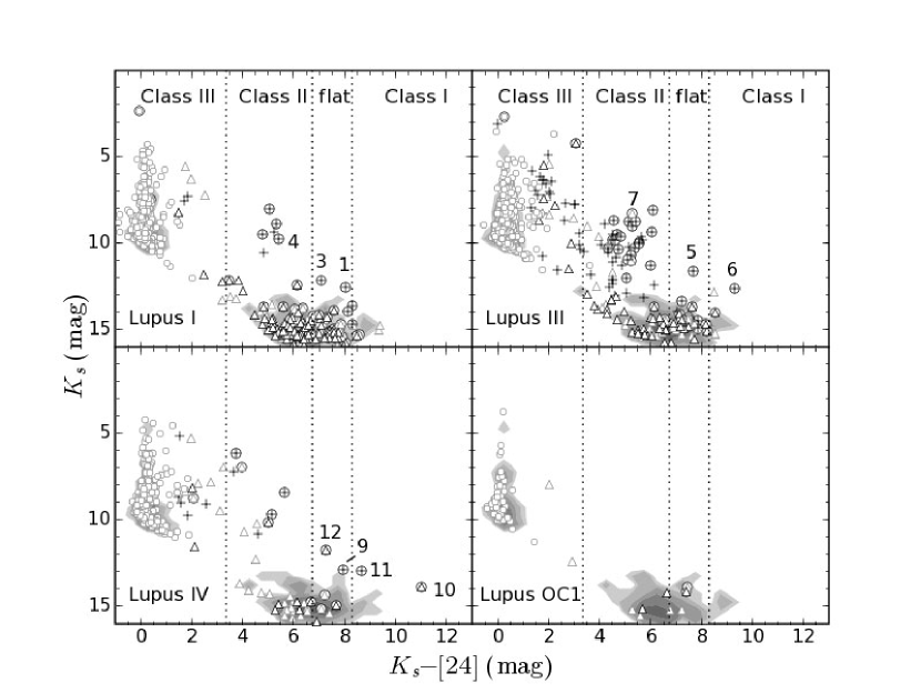
Figure 9.— $K_{s}$ vs. $K_{s}-[24]$ color-magnitude plot for each Lupus region and the SWIRE region. The shaded contours are the counts for the resampled SWIRE region, as described in the text in § 4.2. The contour levels are 1,2,4,8,16, and 32 counts. The data points show the specified Lupus region: I, III, IV, or OC1. Different symbols are used based upon how a source is classified (§ 3.4). Gray circles are stars, crosses represent ‘YSO candidates’, gray triangles are sources only detected at $JHK_{s}$ and $24\>\mu$m wavelengths, and black triangles are all other classifications. Furthermore, a black circle surrounds any source also detected at $70\>\mu$m. The vertical dotted lines show the class boundaries as defined by Greene et al. (1994). The numbers reference sources discussed in § 5.5 and listed in Tables 3 and 4.

Figure 9 shows the $K_{s}$ vs. $K_{s}-[24]$ plot for each cloud region and OC1. We have drawn dotted lines to separate different YSO classes, as defined by Greene et al. (1994). The four YSO classes are determined by the value of $\alpha=\frac{\mathrm{d}\log\lambda F_{\lambda}}{\mathrm{d}\log\lambda}$, the slope of the linear least-squares fit to all data points from $K_{s}-24\>\mu$m. The four classes are as follows: Class I: $\alpha\geq 0.3$; Flat spectrum: $0.3>\alpha\geq-0.3$; Class II: $-0.3>\alpha\geq-1.6$; and Class III: $\alpha<-1.6$. We have included sources with $\alpha=0.3$ into class I since these sources were left undefined by Greene et al. (1994). We expect the SWIRE data should contain nothing but non-YSO stars and background galaxies (see § 4.2). Based on the shaded contours, we can group the sources into roughly one of three regions in this figure: stars are located at $K_{s}-[24]\approx 0$, galaxies are fainter than $K_{s}\sim 13.5$ mag with $K_{s}-[24]$ between 4-10, and YSOs have a $K_{s}-[24]$ color excess and are brighter than $K_{s}\sim 13.5$ mag.

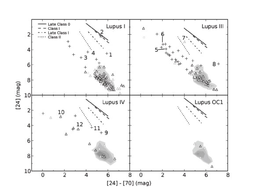
Figure 10.— $[24]$ vs. $[24]-[70]$ color-magnitude plots for each Lupus region. See Figure 9 for a description of the symbols, shaded contours, and numbers. Four protostar models are shown from Whitney et al. (2003). Except for Lupus OC1, we shifted the model tracks to correspond to our assumed distances for each Lupus region.

We have also plotted $[24]$ vs. $[24]-[70]$ for each region (Figure 10). Only the brightest stars should be detected at $70\>\mu$m and in fact we do see just one star, in Lupus III, with $[24]-[70]\approx 0$. Based on the SWIRE contours, we expect that sources with $[24]\gtrsim 6$ mag are likely galaxies, while those brighter than this limit are YSOs. We plotted four YSO model curves from Whitney et al. (2003) showing different stages of evolution. Each curve represents a range of inclinations from pole-on (upper left) to edge-on (lower right). These models assume a distance of $140$ pc, to correspond with nearby star-forming clouds such as Taurus. We shifted the $24\>\mu$m magnitudes in each sub-panel to correspond to our assumed distance for that cloud region. We did not apply a shift to the off-cloud region. With only a few notable exceptions, our ‘YSO candidates’ are bluer than what is predicted by the models.

5.3. Young Stellar Objects

Comerón (2007) has compiled the most up-to-date listing of all known and suspected YSOs in Lupus. Within our observed IRAC+MIPS areas, there are just 5 such objects in Lupus I, 55 in Lupus III, and 3 in Lupus IV. The number of ‘YSO candidates’ identified from our source classification mirrors this distribution; there are 16 ‘YSO candidates’ in Lupus I, 75 in Lupus III, and 12 in Lupus IV. Compared to other c2d clouds such as Perseus, Ophiuchus, and Serpens, Lupus is relatively quiescent; only of one the regions, Lupus III, has significant star formation activity. The number of ‘YSO Candidates’ per square degree is 12, 58, and 33, for Lupus I, III, and IV, respectively. Compared to these values, the number of ‘YSO candidates’ per square degree is $\sim 300$ in Serpens (Harvey et al., 2006), $\sim 100$ in Perseus (Jørgensen et al., 2006), and $\sim 200$ in the L1688 region of Ophiuchus (Allen et al., 2007).

Table 5 YSO Candidate Statistics

	Lupus I	Lupus III	Lupus IV
YSO candidates	16	75	12
YSOs per deg2	12	58	33
Known YSOs ($4\arcsec$)	3 of 5	27 of 55	2 of 3
Class I	5	2	1
Flat Spectrum	2	5	1
Class II	6	45	5
Class III	3	23	5

Note. — Statistics on the number of ‘YSO candidates’ identified in the three Lupus regions based on IRAC and MIPS. See § 3.4 for a discussion of how these sources are defined.

We have compared our ‘YSO candidate’ sample with the list of known and suspected YSOs to see how many of the sources we identify. Our results are summarized in Table 5. Overall, we find a match within $4\arcsec$ for 32 out of the 63 known and suspected YSOs. If we only consider previously known classical T-Tauri stars, we identify 26 out of 40, or about two-thirds. Of the 31 “missed” YSOs, 25 are not in our high-reliability catalogs while the remaining six are not identified as ‘YSO candidates’. In Table 5 we have also broken down our ‘YSO candidates’ by YSO class. For all three cloud regions, the majority of our objects are in the Class II and Class III categories. This result agrees with previous studies that have found a number of T-Tauri stars within the cloud, but no evidence of a large number of Class I and Flat spectrum stars (e.g. Krautter, 1991).

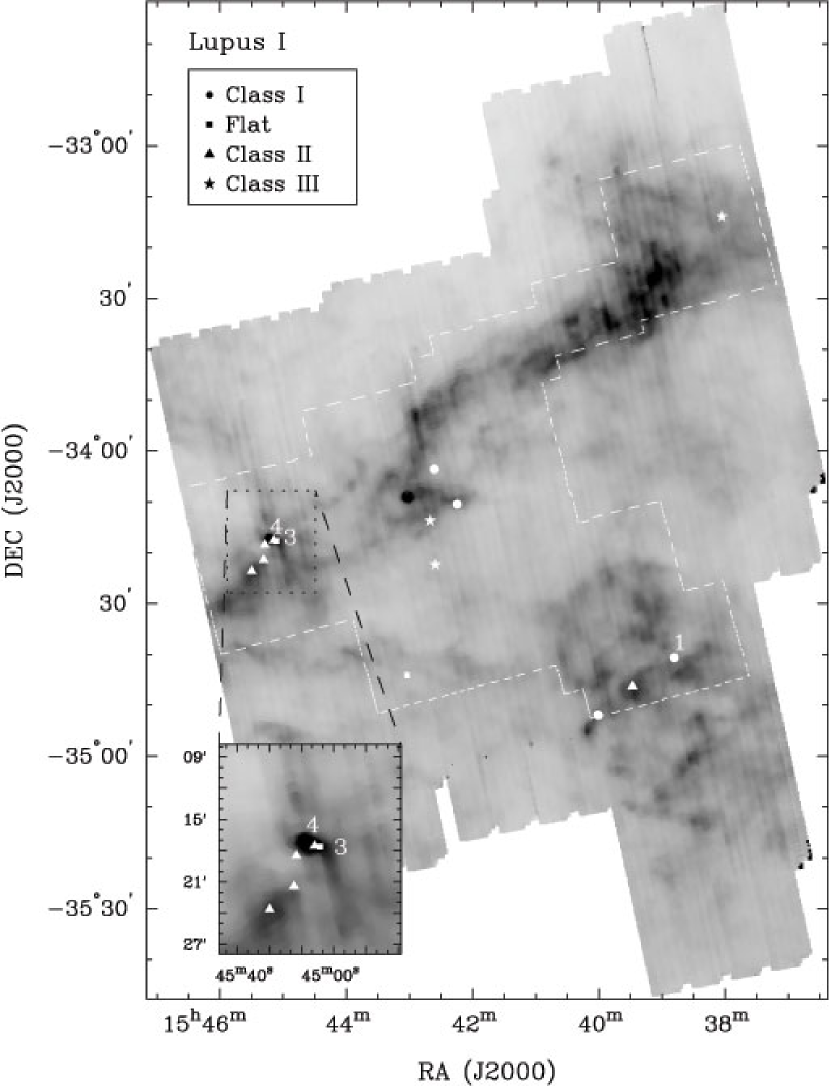
Figure 11.— Lupus I ‘YSO candidates’ overlaid on the $160\>\mu$m image. The four symbols correspond to different YSO classes as noted in the legend and defined in § 5.2. A few sources have been numbered; these are discussed in § 5.5. Since our YSO classification procedures are based on IRAC and MIPS data, we have drawn a white outline to illustrate the area with both IRAC and MIPS observations.

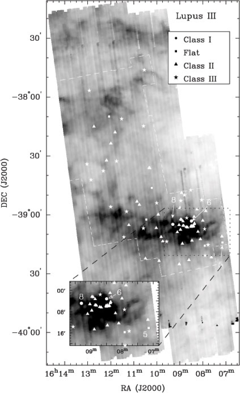
Figure 12.— Lupus III ‘YSO candidates’ overlaid on the $160\>\mu$m image. See Figure 11 for a description of the symbols and their meanings.

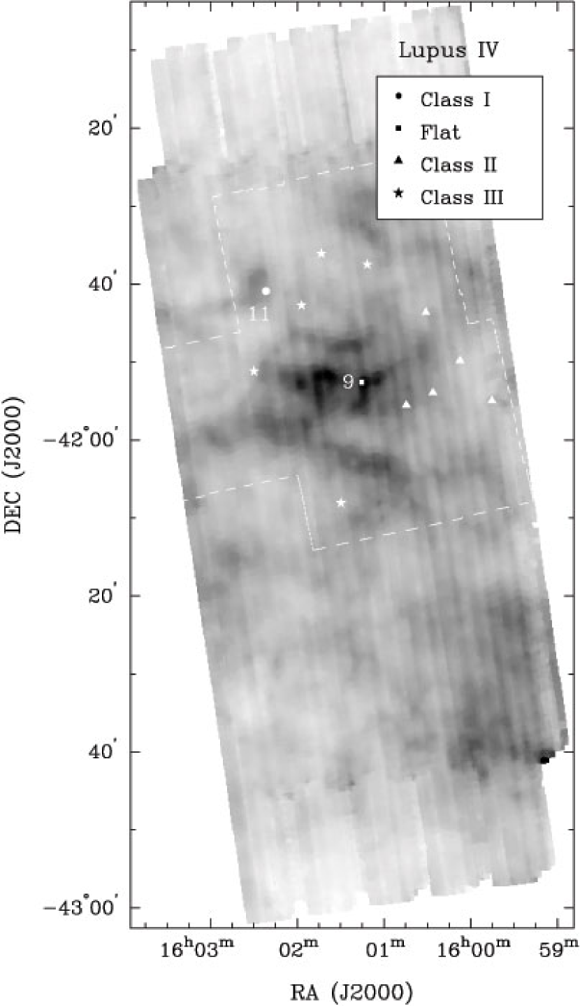
Figure 13.— Lupus IV ‘YSO candidates’ overlaid on the $160\>\mu$m image. See Figure 11 for a description of the symbols and their meanings.

In Figures 11 - 13 we have plotted the positions of all our ‘YSO candidates’ on the $160\>\mu$m emission. Since we require both IRAC and MIPS data to classify ‘YSO candidates’, we have shown the extent of the IRAC observations with white outlines. A few sources have been numbered; these will be discussed in the following section.

5.4. Extinction Maps

To create extinction maps for our observed regions, we started by excluding 2MASS sources with only an upper limit flux in any of the $JHK_{s}$ bands. For the remainder of the 2MASS sources, we calculated $A_{V}$ values from the $JHK_{s}$ bands using the method outlined in § 3.4. Our method gave us pinpoint measurements of the $A_{V}$ along each source’s line-of-sight. We converted these randomly distributed extinction values into uniform maps by creating a $0\farcm 4$ pixel grid on top of the data. At each grid position, the extinction value in that cell equals the weighted average of the extinctions of individual points within a $2^{\prime}$ radius. This average is weighted both by uncertainty in the individual $A_{V}$ values and by distance from the center of the cell with a Gaussian function having a full-width half-maximum (FWHM) equal to $2^{\prime}$. Thus, our maps have $2^{\prime}$ resolution with 5 pixels across the FWHM. We chose this cell size and resolution to have a well-sampled PSF and to ensure that our maps would have an extinction value for every pixel, even in the highest $A_{V}$ regions. The median number of $A_{V}$ values in each cell is roughly 40 for Lupus I, and 80 for Lupus III and IV. The percentage of cells with less than 10 $A_{V}$ values is $1-2$% for all three cloud regions. The extinction contours are shown in Figures 14, 15, 16 overlaid on the $160\>\mu$m emission (grayscale). We subtracted the median off-cloud $A_{V}$, 0.7 mag., from each map. In all three maps, the extinction contours start at 3 magnitudes of $A_{V}$ and increase in steps of 3 mags. There is a strong correspondence between the $160\>\mu$m emission and the $A_{V}$ contours suggesting the $160\>\mu$m emission traces the dust. A detailed comparison of $A_{V}$ and $160\>\mu$m emission is beyond the scope of this paper.

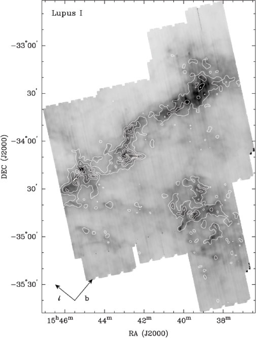
Figure 14.— The magnitudes of visual extinction (contours) are overlaid on the $160\>\mu$m emission map for Lupus I. The contours range from 3 to 15 $A_{V}$, in steps of 3 $A_{V}$. The extinction map has 2 arcminute resolution. We have also shown the direction of increasing Galactic $l$ and b coordinates.

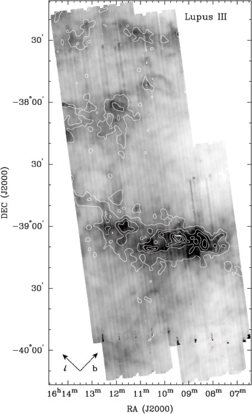
Figure 15.— The magnitudes of visual extinction (contours) are overlaid on the $160\>\mu$m emission map for Lupus III. The contours range from 3 to 18 $A_{V}$, in steps of 3 $A_{V}$. The extinction map has 2 arcminute resolution. We have also shown the direction of increasing Galactic $l$ and b coordinates.

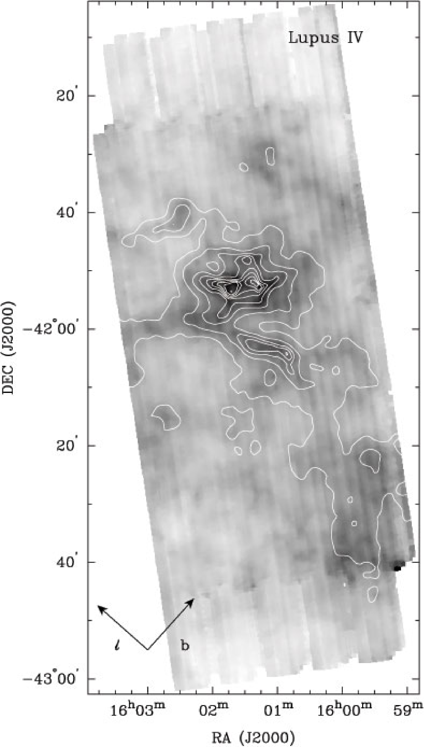
Figure 16.— The magnitudes of visual extinction (contours) are overlaid on the $160\>\mu$m emission map for Lupus IV. The contours range from 3 to 27 $A_{V}$, in steps of 3 $A_{V}$. The extinction map has 2 arcminute resolution. We have also shown the direction of increasing Galactic $l$ and b coordinates.

The mass in each Lupus region was estimated by converting the extinction values in each cell to column density using the equation from Bohlin et al. (1978), assuming $R_{V}=A_{V}/E(B-V)=3.1$:

$$N_{HI}/A_{V}=1.87\times 10^{21}\>\rm{cm}^{2}\>\rm{mag}^{-1}$$ (2)

Note that this relationship was established for the diffuse ISM ($R_{V}=3.1$) and not in dense molecular clouds such as we observed, so this equation may not be valid. This is an important concern since we have used the Weingartner & Draine $R_{V}=5.5$ dust model in this paper (see § 3.4). The data compiled by Kim & Martin (1996) are consistent with $N_{HI}/A_{V}$ being independent of $R_{V}$, albeit with large uncertainties. In this paper, we will use the value of $N_{HI}/A_{V}$ given in Equation 2, but note that this is possible source of error in our final mass estimates.

With this equation, plus the molecular weight per hydrogen molecule, $\mu_{H_{2}}=2.8$ (calculated from Cox, 2000), the mass of a hydrogen atom, and the distance to each Lupus region, we computed masses for each Lupus region from the extinction maps. In Table 2 we list the derived mass in regions with $A_{V}\geq 3$ for each cloud based on our extinction maps.

It is difficult to compare our mass estimates with values in the literature since the mapped areas are not always comparable in size. However, two authors have observed comparable regions in ¹³CO ($J=1\rightarrow 0$) and C¹⁸O ($J=1\rightarrow 0$) (hereafter ¹³CO and C¹⁸O, respectively.) Tachihara et al. (1996) observed Lupus I and III in ¹³CO with $8\arcmin$ resolution and Hara et al. (1999) observed Lupus I, III, and IV in C¹⁸O with a resolution of $2\farcm 6$. Both papers computed cloud masses from emission $\geq 3\sigma$. With the exception of Lupus I, where these authors’ maps extend about 1 degree further to the east, these $\geq 3\sigma$ areas are similar to our $A_{V}\geq 3$ regions. For purposes of comparison to our results, we will scale these authors’ mass estimates using our assumed distances to the Lupus clouds. This only involves changing their mass estimates for Lupus III. We have assumed a distance of 200 pc to this cloud whereas Tachihara et al. (1996) and Hara et al. (1999) assumed a distance of $\sim 150$ pc for all Lupus regions.

The ¹³CO mass in Lupus I is $1200\>M_{\odot}$ which is $\sim 3\times$ larger than our extinction mass of $440\>M_{\odot}$. However, their mapped area is larger than ours and the $3\sigma$ ¹³CO contours cover more area than our $A_{V}\geq 3$ maps. For Lupus III, the ¹³CO mass is $530\>M_{\odot}$, very similar to our extinction mass of $690\>M_{\odot}$. In Lupus I and IV, the C¹⁸O masses agree well with our $A_{V}$ values; the C¹⁸O masses are 327 and 216 $\>M_{\odot}$, respectively, for Lupus I and IV compared to 440 and 250 $\>M_{\odot}$ we derived from $A_{V}$. The only difference is in Lupus III, where our $A_{V}$ mass, $690\>M_{\odot}$, is $3.5\times$ that derived from C¹⁸O ($187\>M_{\odot}$).

Although some differences between our $A_{V}$ mass estimates and those derived from ¹³CO and C¹⁸O exist, there are several possible sources of error that must be considered. Our extinction maps do not cover the exact same areas as the molecular cloud maps which can potentially lead to large differences in mass estimates, as is evident in Lupus I. Furthermore, the molecular masses were estimated assuming a constant excitation temperature of $13$ K, even though measurements of the excitation temperature in individual dense cores in Lupus shown variations (Vilas-Boas, Myers, & Fuller, 2000). Similarly, our $A_{V}$ masses assumed a constant grain composition throughout the clouds. This quantity has also been shown to vary along different sightlines (e.g. Cardelli et al., 1989). Furthermore, our $N_{HI}/A_{V}$ ratio may also be incorrect. A detailed study is needed before making rigorous comparisons between cloud masses derived using various molecular tracers and extinction measurements.

5.5. Selected Sources

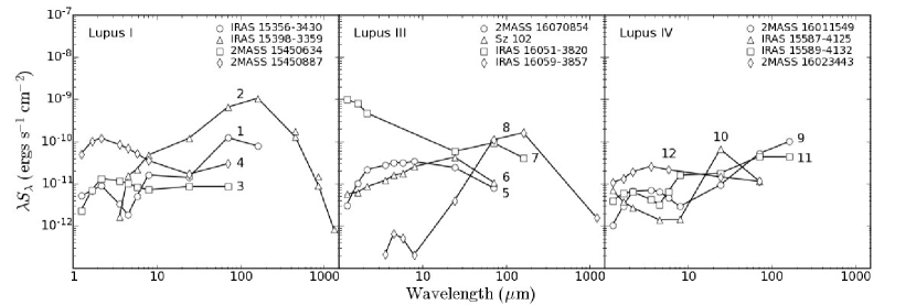
Figure 17.— SEDs of selected sources from the three cloud regions. See § 5.5 for a full discussion of these sources, and Tables 3 and 4 for the positions and fluxes of the sources. We have included sub-millimeter and millimeter wavelength data from the literature for IRAS 15398-3359 and IRAS 16059-3857. For IRAS 15398-3359, the data points at 450 and 850 $\mu$m are from Shirley et al. (2000) with $40\arcsec$ (lower points) and $120\arcsec$ (upper) apertures. The 1.3 mm point comes from Reipurth et al. (1993) with a $23\arcsec$ aperture. The 1.2 mm data point for IRAS 16059-3857 comes from Tachihara et al. (2007).

In this section we highlight a few sources we selected from Figures 9 and 10 that are red relative to the general ‘YSO candidates’ and hence likely to be younger YSOs. From Figure 9 we selected all Flat and Class I sources bright enough in $K_{s}$ to not overlap the shaded SWIRE contours denoting ‘background galaxies’. Furthermore, we selected sources in Figure 10 with $[24]-[70]\geq 4$ and also not overlapping the shaded SWIRE contours. Our final sample consists of 12 objects. These sources are listed in Tables 3 and 4 with positions, fluxes, index numbers, and YSO classification based on $\alpha$. These index numbers are also shown in the color-magnitude plots (Figures 9 - 10), in Figures 11 - 13, showing the location of all ‘YSO candidate’ sources, and in Figure 17, where the SEDs for these objects are plotted.

5.5.1 Lupus I Sources

We selected four sources in Lupus I: one previously known and three objects without references in the literature. The first object is IRAS 15356-3430. The relative brightness of this source in $K_{s}$ places it above the typical extragalactic region in Figure 9. This source is obviously extended in the 2MASS and IRAC bands. Furthermore, it is located in a relatively low extinction region to the south instead of near other known protostars. For these reasons, we believe it to be a background galaxy.

IRAS 15398-3359 is a well-known protostar located in the core B228 (see, e.g. Heyer & Graham, 1989; Shirley et al., 2000, 2002). It has a molecular outflow which was discovered in ¹²CO ($J=2\rightarrow 1$) by Tachihara et al. (1996). There is some correspondence between the Herbig-Haro object HH 185 and the molecular outflow: the blue-shifted velocity lobe from the molecular outflow overlaps the blue-shifted [S II] line from Heyer & Graham (1989). The [S II] line is expected to be excited by the shocks arising from the outflow jet interacting with the ambient medium. In the IRAC images, the protostar appears extended in the same direction as the molecular outflow.

The SED of IRAS 15398-3359 is shown in Figure 17. The data points at 450 and 850 $\mu$m come from Shirley et al. (2000) using their $40\arcsec$ (lower data points) and $120\arcsec$ (upper points) aperture values, while the 1.3 mm point comes from Reipurth et al. (1993) with a $23\arcsec$ aperture. This source does not have a 2MASS detection so it does not appear in Figure 9. It is not classified as a ‘YSO candidate’ because it is saturated at IRAC1 and IRAC2 and therefore was rejected by our YSO classification procedure.

To the east of protostar IRAS 15398-3359 is a cluster of objects with infrared excesses. We have plotted two sources from this region for which we could not find any references in literature. Both are near Sz 68, a known bright T-Tauri star. 2MASS 15450887-3417333 is $\sim 50\arcsec$ away while 2MASS 15450634-3417378 is about $\sim 80\arcsec$ away.

5.5.2 Lupus III Sources

Lupus III contains the most active star forming region in the Lupus cloud complex. HR 5999 dominates the bright nebulous region in the south of our observed region. This source is a well-known Herbig Ae/Be star. Because this source is saturated at $3.6$, $4.5$, and $24\>\mu$m wavelengths, we will not discuss it here. Three of our four sources are nearby, making HR 5999 useful as a location reference.

2MASS 16070854-3914075 exhibits a fairly flat SED indicating a strong IR excess over that of a stellar photosphere. This source is located about $15\arcmin$ to the west of HR 5999. There are several known YSOs in this region, but this source has not been noted in the literature.

Sz 102 is a well-known T-Tauri star located just to the north of the nebulous region containing HR 5999. This source is also known as Th 28 or Krautter’s star. Krautter (1986) discovered an HH outflow from this source (HH 228). There is some evidence for rotation of the jet (Coffey et al., 2004). The SED rises from $1.25-24\>\mu$m, then drops at $70\>\mu$m. This source has also been observed by the c2d program with the Infrared Spectrometer (IRS) from $\sim 5-35\>\mu$m (Kessler-Silacci et al., 2006). The faintness of the object and the orientation of the jet suggest that the source may have an edge-on disk (Hughes et al., 1994). However, the c2d photometry and spectroscopy for this source do not clearly show the double-peaked structure that would be expected for an edge-on disk (e.g. Wood et al., 2002). Stapelfeldt et al. (2007) observed this source with HST and did not see any evidence for an edge-on disk.

Our third source is IRAS 16051-3820. This object is outside of the observed IRAC area, so therefore it cannot be classified as a ‘YSO candidate’. This source does have red $K_{s}-[24]$ and $[24]-[70]$ colors. In Figure 10, this is source #7 and is located between the Late Class I and Class II YSO models. In the 2MASS images, two objects, separated from each other by $\sim 5\arcsec$ are clearly visible. These two objects are not resolved at 24 or $70\>\mu$m. This source has not been previously identified as a ‘YSO candidate’ in the literature.

Lastly, IRAS 16059-3857 is located just to the east of the bright nebulous region. Nakajima et al. (2003) observed this source with $JHK_{s}$ imaging and discovered the region appears as a reflection nebula. They detected an elongated jet-like structure in $K_{s}$ and a fan-shaped structure reminiscent of a cavity created by an outflow. The Herbig-Haro object HH 78 is just to the west. In the IRAC images, this source appears extended in the roughly the same direction as the fan-shaped structure seen by Nakajima et al. (2003). Tachihara et al. (2007) found this source to be embedded in an H¹³CO⁺ core and measured a 1.2 mm continuum PSF flux for it. Because there is no 2MASS data for this source, it does not appear in Figure 9. However, it is reddest source in Figure 10.

5.5.3 Lupus IV Sources

Compared to Lupus III, Lupus IV is a more quiescent region with only a few T-Tauri stars, most of them previously known. We focus on the four reddest objects in Figure 9 that are not within the ‘background galaxy’ region denoted by the SWIRE contours.

2MASS 16011549-4152351 is located near the center of globule filament 17 (GF 17), at approximately the center of the mapped region. This source is consistently rising at all wavelengths longward of $8\>\mu$m and appears to be a deeply embedded protostar in the filament. There is some nebulosity associated with the source at 3.6 and $4.5\>\mu$m.

IRAS 15587-4125 is the reddest source in Figure 9, but has only a modest excess in Figure 10. The SED shows a sharp rise between $8$ and $24$. This source is the known planetary nebula PN G336.9+08.3 (Acker et al., 1992).

IRAS 15589-4132 has an SED that rises rapidly at wavelengths longward of $4.5\>\mu$m. Because this source is extended in all four IRAC bands and in the 2MASS $JHK_{s}$ images, we suspect this source to be a galaxy. This source has no identification in the literature.

Our last source, 2MASS 16023443-4211294, is not identified as a ‘YSO candidate’ because it falls outside of the observed area of IRAC2 ($4.5\>\mu$m) and IRAC4 ($8\>\mu$m). The only reference in the literature for this source is an x-ray source about $12\arcsec$ away. The source does not appear extended in 2MASS, IRAC, or MIPS images. This source is located far from the globular filament, so it tempting to identify this object as a background galaxy. However, the SED for this object is fairly flat, which is consistent with other ‘YSO candidates’ instead of the rising SED found in our suspected galaxies.

6. Summary

We presented maps of three regions within the Lupus molecular cloud complex at 24, 70, and $160\>\mu$m observed with MIPS. We discussed the c2d data reduction pipeline (Evans et al., 2007) and the differences between the c2d pipeline and our catalogs used here. Our catalogs were bandmerged with 2MASS and SED fitting was performed to classify objects. After removing asteroids and selecting only the highest reliability MIPS sources, our final catalogs contain 1790 sources for Lupus I, 1950 for Lupus III, and 770 for Lupus IV. In addition, we have created three c2d processed catalogs from a subset of the ELAIS N1 SWIRE data. Each catalog was trimmed to have similar sensitivity and extinction as each of our cloud regions.

We compared the $24\>\mu$m source counts in each region to our c2d processed SWIRE catalog, a catalog for a nearby off-cloud region, and the star counts derived from the Wainscoat model. We find that Lupus I, at the highest Galactic latitude, shows an excess of sources at fainter fluxes over the Wainscoat model, while III and IV, at more modest latitudes, are consistent with Wainscoat over a broad range of fluxes. The faint Lupus I counts are consistent with the c2d processed SWIRE catalog suggesting this region is more dominated by background galaxies.

Using an empirical method developed by Harvey et al. (2007), we created a sample of objects that is strongly enriched in YSOs and minimizes contamination by background galaxies. We identify 103 ‘YSO candidates’ within the three Lupus regions surveyed. Of these, we find positional matches with 26 of the 40 confirmed classical T-Tauri stars in Lupus and 6 of the suspected protostars from López Martí et al. (2005) and Comerón et al. (2003). When we break down our ‘YSO candidate’ sample by $\alpha$, the best-fit slope to the flux from $2-24\>\mu$m, we find that almost all of the sources fall into the Class II and Class III categories. This suggests that the most of the protostars within Lupus are older and more evolved. There are a few of the younger Class I and Flat spectrum sources in each region.

Our SED fitting procedure also computes the $A_{V}$ for each object. We have used the 2MASS data to construct extinction maps of the three regions and compared them to the $160\>\mu$m emission. Our cloud masses derived from the extinction maps are largely comparable to previous studies, except for Lupus I, where previous authors have mapped a larger region than our observations, and in Lupus III, where our extinction mass is $3.5\times$ larger than the C¹⁸O mass from Hara et al. (1999). However, there are several different factors that could alter these mass estimates such as assumptions about temperature or dust composition. A more detailed study is needed.

Based on two color-magnitude diagrams we selected 12 objects with very red $K_{s}-[24]$ and $[24]-[70]$ colors for individual mention. Three of these are previously known protostars: IRAS 15398-3359, Sz 102, and IRAS 16059-3857. We suspect two other sources of being bright background galaxies, one object is a known planetary nebula, and one object is a double star. We are left with five previously unknown potential protostars. Further observations are needed to confirm whether these sources are bona-fide YSOs.

References

- Acker et al. (1992) Acker, A., Marcout, J., Ochsenbein, F., Stenholm, B., & Tylenda, R. 1992, Garching: European Southern Observatory, 1992
- Allen et al. (2007) Allen, L. E. et al. in preparation
- Bertout et al. (1999) Bertout, C., Robichon, N., & Arenou, F. 1999, A&A, 352, 574
- Bohlin et al. (1978) Bohlin, R. C., Savage, B. D., & Drake, J. F. 1978, ApJ, 224, 132
- Cambrésy (1999) Cambrésy, L. 1999, A&A, 345, 965
- Cardelli et al. (1989) Cardelli, J. A., Clayton, G. C., & Mathis, J. S. 1989, ApJ, 345, 245
- Coffey et al. (2004) Coffey, D., Bacciotti, F., Woitas, J., Ray, T. P., & Eislöffel, J. 2004, ApJ, 604, 758
- Comerón et al. (2003) Comerón, F., Fernández, M., Baraffe, I., Neuhäuser, R., & Kaas, A. A. 2003, A&A, 406, 1001
- Comerón (2007) Comerón, F., 2007, The Lupus Clouds, in Handbook of star forming regions, ed B. Reipurth, Cambridge Univ. Press
- Cox (2000) Cox, A. N. 2000, Allen’s astrophysical quantities, 4th ed. Publisher: New York: AIP Press; Springer, 2000. Edited by Arthur N. Cox. ISBN: 0387987460
- de Zeeuw et al. (1999) de Zeeuw, P. T., Hoogerwerf, R., de Bruijne, J. H. J., Brown, A. G. A., & Blaauw, A. 1999, AJ, 117, 354
- Evans et al. (2003) Evans, N. J., et al. 2003, PASP, 115, 965
- Evans et al. (2007) Evans, N. J., II, Harvey, P. M., Dunham, M. M., Mundy, L. G., Lai, S.,Chapman, N., Huard, T., Brooke, T. Y., & Koerner, D. W., 2007, Delivery of Data from the c2d Legacy Project: IRAC and MIPS (Pasadena, SSC), http://ssc.spitzer.caltech.edu/legacy/original.html
- Fazio et al. (2004) Fazio, G. G., et al. 2004, ApJS, 154, 10
- Franco (1990) Franco, G. A. P. 1990, A&A, 227, 499
- Greene et al. (1994) Greene, T. P., Wilking, B. A., Andre, P., Young, E. T., & Lada, C. J. 1994, ApJ, 434, 614
- Hara et al. (1999) Hara, A., Tachihara, K., Mizuno, A., Onishi, T., Kawamura, A., Obayashi, A., & Fukui, Y. 1999, PASJ, 51, 895
- Harvey et al. (2006) Harvey, P., et al. 2006, ApJ, 644, 307
- Harvey et al. (2007) Harvey, P., et al. 2007a, in press
- Harvey et al. (2007) Harvey, P., et al. 2007b, in press
- Heyer & Graham (1989) Heyer, M. H., & Graham, J. A. 1989, PASP, 101, 816
- Hughes et al. (1994) Hughes, J., Hartigan, P., Krautter, J., & Kelemen, J. 1994, AJ, 108, 1071
- Indebetouw et al. (2005) Indebetouw, R., et al. 2005, ApJ, 619, 931
- Jørgensen et al. (2006) Jørgensen, J., et al. 2006, ApJ, 645, 1246
- Kessler-Silacci et al. (2006) Kessler-Silacci, J., et al. 2006, ApJ, 639, 275
- Kim & Martin (1996) Kim, S.-H., & Martin, P. G. 1996, ApJ, 462, 296
- Koornneef (1983) Koornneef, J. 1983, A&A, 128, 84
- Krautter (1986) Krautter, J. 1986, A&A, 161, 195
- Krautter (1991) Krautter, J. 1991, Low Mass Star Formation in Southern Molecular Clouds, ed. B. Reipurth, ESO Scientific Report, 11, 127
- Krautter et al. (1997) Krautter, J., Wichmann, R., Schmitt, J. H. M. M., Alcala, J. M., Neuhauser, R., & Terranegra, L. 1997, A&AS, 123, 329
- Lai et al. (in prep.) Lai, S.-P., et. al., 2007, in prep.
- López Martí et al. (2005) López Martí, B., Eislöffel, J., & Mundt, R. 2005, A&A, 440, 139
- Makovoz & Marleau (2005) Makovoz, D., & Marleau, F. R. 2005, PASP, 117, 1113
- Nakajima et al. (2003) Nakajima, Y., et al. 2003, AJ, 125, 1407
- Padgett et al. (2007) Padgett, D., et al. 2007, submitted
- Rebull et al. (2007) Rebull, L. M., et al. 2007, ApJS, in press
- Reipurth et al. (1993) Reipurth, B., Chini, R., Krugel, E., Kreysa, E., & Sievers, A. 1993, A&A, 273, 221
- Rieke et al. (2004) Rieke, G. H., et al. 2004, ApJS, 154, 25
- Schechter et al. (1993) Schechter, P. L., Mateo, M., & Saha, A. 1993, PASP, 105, 1342
- Shirley et al. (2000) Shirley, Y. L., Evans, N. J., Rawlings, J. M. C., & Gregersen, E. M. 2000, ApJS, 131, 249
- Shirley et al. (2002) Shirley, Y. L., Evans, N. J., II, & Rawlings, J. M. C. 2002, ApJ, 575, 337
- Stapelfeldt et al. (2007) Stapelfeldt, K. R., et al. 2007, in preparation
- Stapelfeldt et al. (in prep.) Stapelfeldt, K. R., et al., in preparation
- Surace et al. (2004) Surace, J. A., et al. 2004, VizieR Online Data Catalog, 2255, 0
- Tachihara et al. (1996) Tachihara, K., Dobashi, K., Mizuno, A., Ogawa, H., & Fukui, Y. 1996, PASJ, 48, 489
- Tachihara et al. (2007) Tachihara, K., Rengel, M., Nakajima, Y., Yamaguchi, N., André, P., Neuhäuser, R., Onishi, T., Fukui, Y., & Mizuno, A. 2007, ApJ, in press
- Vilas-Boas, Myers, & Fuller (2000) Vilas-Boas, J. W. S., Myers, P. C., & Fuller, G. A. 2000, ApJ, 532, 1038
- Wainscoat et al. (1992) Wainscoat, R. J., Cohen, M., Volk, K., Walker, H. J., & Schwartz, D. E. 1992, ApJS, 83, 111
- Weingartner & Draine (2001) Weingartner, J. C., & Draine, B. T. 2001, ApJ, 548, 296
- Werner et al. (2004) Werner, M. W., et al. 2004, ApJS, 154, 1
- Whitney et al. (2003) Whitney, B. A., Wood, K., Bjorkman, J. E., & Cohen, M. 2003, ApJ, 598, 1079
- Wichmann et al. (1997) Wichmann, R., Krautter, J., Covino, E., Alcala, J. M., Neuhaeuser, R., & Schmitt, J. H. M. M. 1997, A&A, 320, 185
- Wichmann et al. (1998) Wichmann, R., Bastian, U., Krautter, J., Jankovics, I., & Rucinski, S. M. 1998, MNRAS, 301, L39
- Wood et al. (2002) Wood, K., Wolff, M. J., Bjorkman, J. E., & Whitney, B. 2002, ApJ, 564, 887
- Young et al. (2005) Young, K., et al. 2005, ApJ, 628, 283