On the asymptotic behavior of Faber polynomials for domains with piecewise analytic boundary

Abstract

For a function $\psi(w)$ analytic and univalent in $\left\{w:1<|w|<\infty\right\}$ with a simple pole at $\infty$ and a continuous extension to $\{w:|w|\geq 1\}$, we consider the Faber polynomials $F_{n}(z)$, $n=0,1,2,\ldots$, associated to $\psi$ via their generating function $\psi^{\prime}(w)/\left(\psi(w)-z\right)=\sum_{n=0}^{\infty}F_{n}(z)w^{-(n+1)}$. Assuming that $\psi$ maps the unit circle $\mathbb{T}_{1}$ onto a piecewise analytic curve $L$ whose exterior domain has no outward-pointing cusps, and under an additional assumption concerning the “Lehman expansion” of $\psi$ about those points of $\mathbb{T}_{1}$ mapped onto corners of $L$, we obtain asymptotic formulas for $F_{n}$ that yield fine results on the location, limiting distribution and accumulation points of the zeros of the Faber polynomials. The asymptotic formulas are shown to hold uniformly and the exact rate of decay of the error terms involved is provided.

AMS classification: 30E10, 30E15, 30C10, 30C15.

Key words and phrases: Faber polynomials, asymptotic behavior, zeros of polynomials, equilibrium measure, Schwarz reflection principle, conformal map.

1 Introduction

Let $\phi$ be a function with a Laurent expansion at $\infty$ of the form

$$\phi(z)=b_{1}z+b_{0}+\frac{b_{-1}}{z}+\frac{b_{-2}}{z^{2}}+\cdots,\quad b_{1}\not=0,\quad\limsup_{n\to\infty}|b_{-n}|^{1/n}<\infty.$$ (1.1)

The $n$th Faber polynomial $F_{n}(z)$, $n=0,1,\ldots\,$, associated with $\phi$ is the polynomial part of the Laurent expansion at infinity of the function $[\phi(z)]^{n}$.

We shall frequently use the following notation: given $r\geq 0$,

$$\mathbb{T}_{r}:=\{w:|w|=r\},\quad\Delta_{r}:=\{w:r<|w|\leq\infty\}.$$

The inverse function of $\phi$, denoted by $\psi$, is well-defined in a neighborhood of $\infty$, and there is a smallest number $\rho<\infty$ such that $\psi$ has an analytic and univalent continuation to $\Delta_{\rho}\setminus\{\infty\}$. If $\rho=0$, then $\phi$ is linear and $F_{n}(z)=(b_{1}z+b_{0})^{n}$. Being this case a trivial one, we assume hereafter that $\phi$ has been normalized so that $\rho=1$.

Then, the function $\psi$ maps $\Delta_{1}$ conformally onto a simply-connected domain $\Omega$, and consequently, $\phi$ has a conformal extension to $\Omega$, with $\phi(\Omega)=\Delta_{1}$. Conversely, by the Riemann mapping theorem, given any simply-connected neighborhood $\Omega$ of $\infty$ whose boundary contains more than one point, there is, up to a multiplicative unimodular constant, a unique conformal map $\phi$ of $\Omega$ onto $\Delta_{1}$ that complies with (1.1). Hence, Faber polynomials are often introduced as being generated by simply-connected neighborhoods of $\infty$.

The function (in the variable $w$) $\psi^{\prime}(w)/\left(\psi(w)-z\right)$ is called the generating function of the Faber polynomials, since as shown by Faber [4] (see also [20]), its Laurent expansion at $\infty$ is

$$\frac{\psi^{\prime}(w)}{\psi(w)-z}=\sum_{n=0}^{\infty}\frac{F_{n}(z)}{w^{n+1}}.$$ (1.2)

By an application of Cauchy integral formula, (1.2) yields the following integral representation for the Faber polynomials: for every $R>1$ and $z$ lying in the interior of the level curve $L_{R}:=\{\psi(w):|w|=R$},

$$F_{n}(z)=\frac{1}{2\pi i}\oint_{\mathbb{T}_{R}}\frac{t^{n}\psi^{\prime}(t)dt}{\psi(t)-z}\,,$$ (1.3)

while for $z$ lying in the exterior of $L_{R}$,

$$F_{n}(z)=[\phi(z)]^{n}+\frac{1}{2\pi i}\oint_{\mathbb{T}_{R}}\frac{t^{n}\psi^{\prime}(t)dt}{\psi(t)-z}.$$ (1.4)

It this paper we investigate the asymptotic behavior of the Faber polynomials and their zeros for certain domains $\Omega$ that are bounded by piecewise analytic curves. Hence the title of this paper. More precisely, we consider domains (or equivalently, functions $\psi$) satisfying assumptions A.1 and A.2 to be stated in what follows.

We define an analytic arc as being the image of the interval $[0,1]$ by a function $f(t)$ analytic in $[0,1]$ such that $f^{\prime}(t)\not=0$ for all $t\in[0,1]$ and $f(t_{1})\not=f(t_{2})$ for all $0<t_{1}<t_{2}<1$. The endpoints of the arc are $f(0)$ and $f(1)$, which may coincide. We call the arc simple if $f$ is one-to-one on $[0,1]$. Notice that, according to this definition, an analytic Jordan curve is also an analytic arc. Our first assumption is:

1. The map $\psi$ has a continuous extension to $\overline{\Delta}_{1}$ and there are $s\geq 1$ distinct points $\omegaup_{1},\omegaup_{2},\ldots,\omegaup_{s}$ in $\mathbb{T}_{1}$ such that if $\ell$ is any of the $s$ open circular arcs that compose $\mathbb{T}_{1}\setminus\{\omegaup_{1},\omegaup_{2},\ldots,\omegaup_{s}\}$, say with endpoints $\omegaup_{k}$, $\omegaup_{j}$, then $\psi$ is one-to-one on $\ell$ and $\psi\left(\overline{\ell}\right)$ is an analytic arc with endpoints $\psi(\omegaup_{k})$, $\psi(\omegaup_{j})$ (see Figure 1).

Figure 1: Illustration of a map $\psi$ satisfying conditions A.1 and A.2.

Thus, $\partial\Omega$ is a piecewise analytic curve that we denote by $L$. Let $z\in L$ and $w=e^{i\Theta}$ be such that $z=\psi(w)$. The exterior angle at $z$ relative to $w$ is defined to be that angle $\alpha\in[0,2\pi]$ such that

$$\arg\left[\psi\left(e^{i\theta}\right)-z\right]\to\left\{\begin{array}[]{ll}\beta&\ \,\mathrm{as}\ \theta\to\Theta-\,,\\ \beta+\alpha&\ \,\mathrm{as}\ \theta\to\Theta+\,.\end{array}\right.$$

Let

$$z_{k}:=\psi(\omegaup_{k}),\quad k\in\{1,2,\ldots,s\}.$$

These points $z_{k}$ will be called the corners of $L$. Notice that they are not necessarily pairwise distinct.

For each $k\in\{1,2,\ldots,s\}$, let $\lambda_{k}\in[0,2]$ be such that $\lambda_{k}\pi$ is the exterior angle at $z_{k}$ relative to $\omegaup_{k}$. It is well-known that when $\lambda_{k}>0$, the mapping $\psi$ has an asymptotic expansion about $\omegaup_{k}$ in functions of the form

$$(w-\omegaup_{k})^{l+j\lambda_{k}}(\log(w-\omegaup_{k}))^{m}\,,\quad w\in\mathbb{C}\setminus\{t\omegaup_{k}:t\leq 1\},$$ (1.5)

with $l\geq 0$, $j\geq 1$, and $m\geq 0$ integers (see [15] and also [17, pp. 57-58]). We will refer to it as the Lehman expansion of $\psi$ about $\omegaup_{k}$ and its exact meaning is explained in Section 4 below. Logarithmic terms (i.e., functions of the form (1.5) with $m\geq 1$) may occur in the expansion only if $\lambda_{k}$ is a rational number. Our second assumption on $\psi$ is:

1. $\lambda_{k}>0$ for every $k\in\{1,2,\ldots,s\}$, and if $\lambda_{k}\in\{1,2\}$ for all $k\in\{1,2,\ldots,s\}$, then there is at least one $k$ for which logarithmic terms occur in the Lehman expansion of $\psi$ about $\omegaup_{k}$.

If $\lambda_{k}\not\in\{1,2\}$, then $\omegaup_{k}$ is a singularity of $\psi$, and a sufficient condition for an $\omegaup_{k}$ with $\lambda_{k}\in\{1,2\}$ to be a singularity of $\psi$ is precisely that logarithmic terms occur in the Lehman expansion of $\psi$ about $\omegaup_{k}$. We do not know whether this condition is also necessary. If that were the case, we could simply rephrase A.2 by saying that all the $\lambda_{k}$’s are positive and at least one $\omegaup_{k}$ is a singularity of $\psi$.

Let us then consider a map $\psi$ satisfying A.1 and A.2. The letter $G$ will denote the complement of $\overline{\Omega}$, so that if $L$ is a Jordan curve, $G$ is the interior domain of $L$.

A first observation is that the asymptotic behavior of $F_{n}$ in $\Omega$ is already given by the integral representation (1.4): for arbitrary $1<R<r$,

$$F_{n}(z)=[\phi(z)]^{n}\left[1+\mathcal{O}\left(\frac{r^{n}}{R^{n}}\right)\right]\,,$$ (1.6)

uniformly on $\psi\left(\overline{\Delta}_{r}\right)$ as $n\to\infty$. Hence, every closed subset of $\Omega$ will be free of zeros of $F_{n}$ for $n$ large enough, and all accumulation points of the zeros of the Faber polynomials must be contained in $\overline{G}$.

Formula (1.6) has been previously extended to $L$ in the pointwise sense, under the additional assumption that $L$ is a Jordan curve. In this case $\phi$ has a continuous extension to $L$ and a more general result of Pritsker [18, Thm. 1.1] about the behavior of weighted Faber polynomials implies that if $z\in L$ is not a corner, then

$$F_{n}(z)=[\phi(z)]^{n}(1+o(1)),\quad(n\to\infty)$$ (1.7)

while for every corner $z_{k}$,

$$F_{n}(z_{k})=\lambda_{k}[\phi(z_{k})]^{n}(1+o(1)),\quad(n\to\infty).$$ (1.8)

The behavior of $F_{n}$ in $G$ has remained quite unknown, but at least for $L$ a piecewise analytic Jordan curve without cusps, Gaier [5] was able to derive uniform estimates on the decrease of $F_{n}$ of the form

$$F_{n}(z)=\mathcal{O}\left(n^{-\lambda}\right),\quad z\in G,$$ (1.9)

where $\lambda$ is the smallest of the exterior angles at the corners of $L$.

In this paper we much improve these results by providing asymptotic formulas for $F_{n}$ that do not require $L$ to be a Jordan curve and that hold uniformly on closed subsets of the complex plane. Moreover, our estimates for the rate of decay of the error terms involved are, in general, best possible. Theorems 2.3, 2.4 and 2.5 of Section 2 are the strengthened versions of (1.6), (1.7) and (1.8), while Theorem 2.1 transparently describes the behavior of $F_{n}$ in $G$, yielding, in particular, Gaier’s estimate (1.9). Theorem 2.1 also shows that the pointwise estimates given by Gaier in [5, Thm. 2] indeed hold locally uniformly on $G$.

As for the zeros of $F_{n}$, the fact that the map $\psi$ under consideration has a singularity on $\mathbb{T}_{1}$ implies, by a general result of Ullman [20, Thm. 1], that all points of $L$ are accumulation points of the zeros of the Faber polynomials. A later complement to Ullman’s results by Kuijlaars and Saff [14, Thms. 1.3, 1.4] implies that there is always a subsequence of the sequence $\{\nu_{n}\}_{n\geq 1}$ of normalized counting measures of the zeros of the $F_{n}$’s that converges in the weak*-topology to the equilibrium measure $\mu_{L}$ of $L$, and this is true of the entire sequence provided that $G=\emptyset$ (see (3.5) and (3.6) in Section 3 for definitions of $\nu_{n}$ and $\mu_{L}$).

We will be able to say much more. In Section 3 we show that, independently of whether $G$ is connected or not, there is always a subsequence of $\{\nu_{n}\}_{n\geq 1}$ that converges in the weak*-sense to $\mu_{L}$. In fact, under an additional assumption that is naturally satisfied in a large number of cases (including when $L$ is a Jordan curve), we prove that compact subsets of $G$ contain at most a finite (independent of $n$) number of zeros of every $F_{n}$, forcing the whole sequence $\{\nu_{n}\}_{n\geq 1}$ to converge to $\mu_{L}$. Furthermore, under that assumption we are also able to characterize those points of $G$ that are accumulation points of the zeros of Faber polynomials.

Faber polynomials for particular domains of the complex plane has been the subject of many recent works, in several of which the boundary of the domain is precisely a piecewise analytic curve, for example, $m$-stars [1], [13], circular lunes [9], $m$-fold symmetric curves and certain lemniscates [10], annular and circular sectors [6], [7]. Our results apply to all these examples.

The rest of this paper is organized as follows. Section 2 presents the asymptotic formulas for Faber polynomials, in Section 3 we draw some conclusions on their zero behavior and analyze two concrete examples. In Section 4 we discuss in detail the Lehman expansion of the exterior map $\psi$, and finally in Sections 5 and 6 we prove all the results.

2 Asymptotic behavior of $F_{n}(z)$

Recall that we are considering a map $\psi$ satisfying assumptions A.1 and A.2 stated in the introduction. Let $\Theta_{1},\Theta_{2},\ldots,\Theta_{s}$ be the arguments of the numbers $\omegaup_{k}$, that is,

$$\omegaup_{k}=e^{i\Theta_{k}},\quad 0\leq\Theta_{k}<2\pi,\quad 1\leq k\leq s\,.$$

Assumption A.2 is independent of the branches chosen for the functions in (1.5) in a $\delta$-neighborhood of the form $\{w\in\Delta_{1}:0<|w-\omegaup_{k}|<\delta\}$. However, to simplify the statements of our results, we choose those corresponding to the branch of the argument

$$\Theta_{k}-\pi<\arg(w-\omegaup_{k})<\Theta_{k}+\pi,\quad w\in\mathbb{C}\setminus\{t\omegaup_{k}:t\leq 1\}.$$

We shall say that $\omegaup_{k}$ is relevant if either $\lambda_{k}\not\in\{0,1,2\}$, or if $\lambda_{k}\in\{1,2\}$ and logarithmic terms occur in the expansion of $\psi$ about $\omegaup_{k}$. With this definition, condition A.2 states that all $\lambda_{k}$’s are positive and that there is at least one relevant $\omegaup_{k}$.

Let now $v\geq 1$ be the number of relevant $\omegaup_{k}$’s. Hereafter we shall assume that the $\omegaup_{k}$’s have been indexed in such a way that $\omegaup_{1},\omegaup_{2},\ldots,\omegaup_{v}$ are precisely the relevant ones. The following weaker version of the Lehman expansion of $\psi$ about a relevant $\omegaup_{k}$ is sufficient to state our main results.

If $k\in\{1,2,\ldots,v\}$ is such that $\lambda_{k}\not\in\{1,2\}$, then there is $A_{k}\not=0$ such that as $w\to\omegaup_{k}$ from the exterior of the unit circle,

$$\psi(w)=z_{k}+A_{k}(w-\omegaup_{k})^{\lambda_{k}}\left(1+o(1)\right),$$ (2.1)

while if $k\in\{1,2,\ldots,v\}$ is such that $\lambda_{k}\in\{1,2\}$, then there exist positive integers $r_{k},\,m_{k}$ with $r_{k}\geq\lambda_{k}$ and $1\leq m_{k}\leq\lfloor r_{k}/\lambda_{k}\rfloor$, and complex numbers $A_{k}\not=0$, $c^{k}_{0}\not=0$, $c^{k}_{1},c^{k}_{2},\ldots,c^{k}_{r_{k}-1}$, such that as $w\to\omegaup_{k}$ from the exterior of the unit circle,

$$\psi(w) = z_{k}+\sum_{l=0}^{r_{k}-1}c^{k}_{l}(w-\omegaup_{k})^{\lambda_{k}+l}+A_{k}(w-\omegaup_{k})^{r_{k}+\lambda_{k}}\left(\log(w-\omegaup_{k})\right)^{m_{k}}\left(1+o(1)\right).$$ (2.2)

From relations (2.1) and (2.2), we associate to each relevant $\omegaup_{k}$ ($1\leq k\leq v$) the number $A_{k}$, the numbers $r_{k}$ and $m_{k}$ whenever $\lambda_{k}\in\{1,2\}$, and the following pair:

$$(\Lambda_{k},M_{k}):=\left\{\begin{array}[]{cc}(\lambda_{k},0),&\ \mathrm{if}\ \lambda_{k}\not\in\{1,2\},\\ (r_{k}+\lambda_{k},m_{k}-1),&\ \mathrm{if}\ \lambda_{k}\in\{1,2\}.\end{array}\right.$$

Observe that $\Lambda_{k}\geq 2$ if $\lambda_{k}\in\{1,2\}$. We will say that $(\Lambda_{k},M_{k})<(\Lambda_{j},M_{j})$ if either $\Lambda_{k}<\Lambda_{j}$, or $\Lambda_{k}=\Lambda_{j}$ and $M_{k}>M_{j}$.

By reindexing the relevant $\omegaup_{k}$’s if needed, we may assume that $\omegaup_{1},\ldots,\omegaup_{v}$ are such that

$$\left(\Lambda_{1},M_{1}\right)=\cdots=\left(\Lambda_{u},M_{u}\right)<\left(\Lambda_{u+1},M_{u+1}\right)\leq\cdots\leq\left(\Lambda_{v},M_{v}\right),$$

for some $u\in\{1,2,\ldots,v\}$.

For any two integers $n,\,m\geq 0$ and a real $\beta>-1$, we define

$$\alpha_{\beta,m}(n):=\int_{0}^{1}x^{n}(1-x)^{\beta}\left(\log(1-x)\right)^{m}dx\,.$$ (2.4)

Then,

$$\alpha_{\beta,m}(n) = \frac{\Gamma(\beta+1)n!(-\log n)^{m}\left[1+\mathcal{O}\left(1/\log n\right)\right]}{\Gamma(n+\beta+2)}$$

$$= \frac{\Gamma(\beta+1)(-\log n)^{m}(1+o(1))}{n^{\beta+1}}$$

as $n\to\infty$.

Recall that we have defined $L:=\partial\Omega$ and $G:=\mathbb{C}\setminus\overline{\Omega}$. We first consider the behavior of $F_{n}$ on $G$.

Theorem 2.1.

Let 

$$\mathcal{C}_{1}:=\left\{\begin{array}[]{ll}[\Gamma(-\lambda_{1})\Gamma(\lambda_{1})]^{-1},&\quad if\ \lambda_{1}\not\in\{1,2\},\\ (-1)^{\Lambda_{1}-1}m_{1}\Lambda_{1},&\quad if\ \lambda_{1}\in\{1,2\}.\end{array}\right.$$

Then, for every $z\in G$,

$$\frac{F_{n}(z)}{\alpha_{\Lambda_{1}-1,M_{1}}(n)}=\mathcal{C}_{1}\sum_{k=1}^{u}\frac{A_{k}e^{i(n+\Lambda_{1})\Theta_{k}}}{z-z_{k}}+R_{n}(z),$$ (2.6)

where $R_{n}(z)$ converges to zero locally uniformly on $G$.

Remark 2.2.

Since some of the $z_{k}$’s may coincide, it is possible that for some subsequence $\{n_{j}\}\subset\mathbb{N}$, the rational functions $\sum_{k=1}^{u}A_{k}e^{i(n_{j}+\Lambda_{1})\Theta_{k}}/(z-z_{k})$ occurring in (2.6) be (or at least converge to) the constant zero function (see the example discussed at the end of Section 3). Nevertheless, as we show with that example (see Theorem 3.9 and its proof), in a situation like this we could still be successful in proving that, after proper normalization, $\{F_{n_{j}}\}$ behaves like certain sequence of rational functions that do not approach zero. The proof can be attempted as follows: write (1.3) as in (5.34), then combine identity (5.14) with the Lehman expansion of $\psi$ about $\omegaup_{k}$ to obtain, for each of the integrals under the $\Sigma$ sign of (5.34), subsequent terms of its expansion as a sum of rational functions whose denominators are powers of $(z-z_{k})$.

Let us now turn our attention to $\overline{\Omega}$. For every $z\in\overline{\Omega}$, let $\eta(z)$ be the (finite) number of elements of the set $\left\{w\in\overline{\Delta}_{1}:\psi(w)=z\right\}$. These elements will be denoted by

$$\phi_{1}(z),\phi_{2}(z),\ldots,\phi_{\eta(z)}(z),$$

being irrelevant the order in which they are numerated. Of course, $\eta(z)=1$ and $\phi_{1}(z)=\phi(z)$ for $z\in\Omega$.

Because $\Omega$ has no outward-pointing cusps, if $z\in L$ and two elements of $\{w\in\mathbb{T}_{1}:\psi(w)=z\}$ belong to $\mathbb{T}_{1}\setminus\{\omegaup_{1},\ldots,\omegaup_{s}\}$, then indeed $\eta(z)=2$. Hence, $1\leq\eta(z)\leq s+1$, and when $z$ is not a corner, $\eta(z)\leq 2$.

For every $z\in L$ and $1\leq j\leq\eta(z)$, let $\hat{\lambda}_{j}(z)\pi$ ($0<\hat{\lambda}_{j}(z)\leq 2$) be the exterior angle at $z$ relative to $\phi_{j}(z)$. Then, only if $z$ is a corner of $L$ it is possible to have $\hat{\lambda}_{j}(z)\not=1$ for some $1\leq j\leq\eta(z)$. Let us define

$$L_{1}:=\left\{z\in L:\eta(z)=1,\ \hat{\lambda}_{1}(z)=1\right\},$$ (2.7)

$$L_{2}:=\left\{z\in L:\eta(z)=2,\ \hat{\lambda}_{1}(z)=\hat{\lambda}_{2}(z)=1\right\}\cup\left\{z_{k}:\lambda_{k}=2\right\}\,.$$ (2.8)

Observe that

$$L=L_{1}\cup L_{2}\cup\{z_{1},\ldots,z_{s}\}.$$

Let $\Phi_{n}:\overline{\Omega}\to\overline{\mathbb{C}}$ be defined by

$$\Phi_{n}(z):=\left\{\begin{array}[]{ll}\underset{}{[\phi(z)]^{n}}\,,&\ \,\ z\in\Omega,\\ {\displaystyle\sum_{j=1}^{\eta(z)}\hat{\lambda}_{j}(z)[\phi_{j}(z)]^{n}}\,,&\ \,\ z\in L.\end{array}\right.$$

Theorem 2.3.

For every $z\in\overline{\Omega}$,

$$F_{n}(z)=\Phi_{n}(z)+R_{n}(z),$$ (2.9)

where $R_{n}(z)$ is such that

1. if $E$ is a closed set and either $E\subset\Omega\cup L_{1}$ or $E\subset L_{2}$, then $R_{n}(z)=\mathcal{O}\left(n^{-\Lambda^{*}}(\log n)^{M^{*}}\right)$ uniformly as $n\to\infty$ on $E$, where $(\Lambda^{*},M^{*})$ is the smallest element of the set

   $$\left\{(\Lambda_{1},M_{1})\right\}\cup\left\{(r_{k},M_{k}):1\leq k\leq u,\ z_{k}\in E\right\};$$

2. for $j=1,2,\ldots,s$, $R_{n}(z_{j})=\mathcal{O}\left(n^{-\Lambda^{*}_{j}}(\log n)^{M^{*}_{j}}\right)$ as $n\to\infty$, where $(\Lambda^{*}_{j},M^{*}_{j})$ is the smallest element of the set

   $$\left\{(\Lambda_{1},M_{1})\right\}\cup\left\{(r_{k},M_{k}):\psi(\omegaup_{k})=z_{j},\ \lambda_{k}\in\{1,2\}\right\}.$$

We can be more specific for closed subsets of $\Omega\cup L_{1}$ or $L_{2}$ without corners.

Theorem 2.4.

Let $E\subset\left(\Omega\cup L_{1}\right)\setminus\{z_{1},\ldots,z_{s}\}$ be a closed set. There exists an open set $U\supset E$ such that $\phi$ has an analytic and univalent continuation to $U$ and

$$F_{n}(z)=[\phi(z)]^{n}+\alpha_{\Lambda_{1}-1,M_{1}}(n)\left(\mathcal{C}_{1}\sum_{k=1}^{u}\frac{A_{k}e^{i(n+\Lambda_{1})\Theta_{k}}}{z-z_{k}}+R_{n}(z)\right),$$ (2.10)

with $R_{n}(z)\to 0$ uniformly on $U$ as $n\to\infty$.

Let now $E\subset L_{2}\setminus\{z_{1},\ldots,z_{s}\}$ be a simple analytic arc. Then, there is a “strip-like” connected neighborhood $U$ of $E$ such that $\overline{U}\cap L$ is a simple analytic arc contained in $L_{2}$, $U\setminus L$ consists of two open components $U^{+}$, $U^{-}$, both contained in $\Omega$, and if $z^{*}$ denotes the Schwarz reflection of $z$ about the analytic arc $E$, then $z^{*}\in U^{\pm}$ if and only if $z\in U^{\mp}$.

Let $\phi_{+}$, $\phi_{-}$ be the restrictions of $\phi$ to $U^{+}$, $U^{-}$, respectively. Each of these functions is continuous along the arc $U\cap L$, mapping it onto an arc of the unit circle. By the Schwarz reflection principle [3], each function has an analytic and univalent continuation to all of $U$, whose values on $U^{\pm}$ are given by

$$\phi_{\pm}(z)=\frac{1}{\overline{\phi_{\pm}(z^{*})}},\quad z\in U^{\mp}.$$

Theorem 2.5.

Let $E\subset L_{2}\setminus\{z_{1},\ldots,z_{s}\}$ be a simple analytic arc. There exists a neighborhood $U$ of $E$ as described above such that for all $z\in U$,

$$F_{n}(z)=[\phi_{+}(z)]^{n}+[\phi_{-}(z)]^{n}+\alpha_{\Lambda_{1}-1,M_{1}}(n)\left(\mathcal{C}_{1}\sum_{k=1}^{u}\frac{A_{k}e^{i(n+\Lambda_{1})\Theta_{k}}}{z-z_{k}}+R_{n}(z)\right),$$ (2.11)

with $R_{n}(z)\to 0$ uniformly on $U$ as $n\to\infty$.

Remark 2.6.

1) Concerning how fast the error terms $R_{n}(z)$ in (2.6), (2.10) and (2.11) approach zero, the best it can be said, in general, is that they decrease at least as fast as the dominant terms in the right-hand side of (5.36) in page 5.36, where the rate of decay of the functions $r_{\sigma_{k},n}(z)$ therein is estimated in the table of Remark 5.4 in page 5.4.

2) The estimates provided in Theorem 2.3 for $R_{n}(z)$ are also best possible, as can be verified from relation (5.58) for part (a), and from relation (5.65) for part (b).

3 The zeros of $F_{n}(z)$

In this section we draw from our previous results some conclusions about the location, accumulation points and limiting distribution of the zeros of Faber polynomials.

From Theorem 2.3 we immediately see that

$$\lim_{n\to\infty}\frac{F_{n}(z)}{\Phi_{n}(z)}=1$$ (3.1)

locally uniformly on $\Omega\cup L_{1}$, where $\Phi_{n}|_{\Omega\cup L_{1}}$ is simply the continuous extension of $[\phi(z)]^{n}$ to $\Omega\cup L_{1}$. Hence, we have

Corollary 3.1.

For every closed set $E\subset\Omega\cup L_{1}$, there is a number $N_{E}$ such that when $n>N_{E}$, $F_{n}(z)$ has no zeros on $E$.

Let us now focus on the effect that Theorem 2.1 has on the zeros of $F_{n}$. It is interesting that asymptotic formulas similar to (2.6) are also satisfied by orthogonal polynomials on the unit circle with respect to certain types of weights. Some of the results that follow are basically known consequences of such type of behavior, see e.g., [22], [16].

We first rewrite (2.6) in a more suitable way. Put

$$\hat{A}_{k}:=A_{k}e^{i\Lambda_{1}(\Theta_{k}-\Theta_{1})}\,,\quad 1\leq k\leq u\,,$$

and let $\theta_{1},\theta_{2},\ldots,\theta_{u}$ be such that

$$e^{2\pi i\theta_{k}}=e^{i(\Theta_{k}-\Theta_{1})},\quad\theta_{k}\in(0,1],\quad 1\leq k\leq u\,,$$

so that (2.6) takes the form

$$F^{*}_{n}(z)=H_{n}(z)+o(1)$$ (3.2)

locally uniformly on $G$ as $n\to\infty$, where

$$F_{n}^{*}(z)=\left[\mathcal{C}_{1}e^{i(n+\Lambda_{1})\Theta_{1}}\alpha_{\Lambda_{1}-1,M_{1}}(n)\right]^{-1}F_{n}(z)\,,\quad H_{n}(z)=\sum_{k=1}^{u}\frac{\hat{A}_{k}e^{2\pi in\theta_{k}}}{z-z_{k}}\,.$$ (3.3)

In view of (3.2) and the form of the rational functions $H_{n}$, the sequence $\{F_{n}^{*}\}_{n\geq 1}$ is a normal family on $G$, and a function $f$ is the uniform limit on $G$ of some subsequence $\left\{F_{n_{j}}^{*}\right\}_{j\geq 1}$ if and only if it is the uniform limit of $\left\{H_{n_{j}}\right\}_{j\geq 1}$. Hence, every such $f$ must have the form

$$f(z)=\sum_{k=1}^{u}\frac{\hat{A}_{k}e^{2\pi i\vartheta_{k}}}{z-z_{k}}.$$ (3.4)

Because the $z_{k}$’s are not necessarily pairwise distinct, some of these limit functions can be identically zero, which makes Theorem 2.1 insufficient to describe the zeros of the $F_{n}$’s. Therefore, we shall often make the assumption that

1. no subsequence of $\{H_{n}\}_{n\geq 0}$ converges to the null function.

If A.3 is satisfied, then all uniform limit points of $\{F^{*}_{n}\}_{n\geq 0}$ are nonzero rational functions of bounded degree. Let us see what this implies on the limiting distribution of the zeros of $F_{n}$.

Let $\nu_{n}$ be the normalized counting measure of the zeros of $F_{n}$, that is,

$$\nu_{n}:=n^{-1}\sum_{k=1}^{n}\delta_{z_{k,n}}\,,\quad n=1,2,\ldots,$$ (3.5)

where $z_{1,n},z_{2,n},\ldots,z_{n,n}$ are the zeros of $F_{n}$ (counting multiplicities) and $\delta_{z}$ is the unit point measure at $z$.

A subsequence $\{\nu_{n_{j}}\}_{j\geq 1}$ of $\{\nu_{n}\}_{n\geq 1}$ is said to converge in the weak*-topology to a Borel measure $\mu$ (symbolically, $\nu_{n_{j}}\overset{*}{\longrightarrow}\mu$ as $j\to\infty$) if for every continuous function $f$ defined on $\overline{\mathbb{C}}$, $\lim_{j\to\infty}\int f\nu_{n_{j}}=\int f\mu$.

Let $\mu_{L}$ be the equilibrium measure of $L$, i.e., the measure supported on $L$ whose value at any given Borel set $B\subset L$ is

$$\mu_{L}(B)=\frac{1}{2\pi}\int_{B^{-1}}|dt|,\quad B^{-1}:=\{t\in\mathbb{T}_{1}:\psi(t)\in B\}.$$ (3.6)

Notice that $\mu_{L}$ is a probability measure whose support is $L$.

Corollary 3.2.

Assume that A.3 holds. Then, for every closed set $E\subset G$ there is a number $N_{E}$ such that when $n>N_{E}$, $F_{n}(z)$ has at most $J-1$ zeros in $E$ (counting multiplicities), where $J$ is the number of corners $z_{k}$. Hence, $\nu_{n}\overset{*}{\longrightarrow}\mu_{L}$ as $n\to\infty$.

Remark 3.3.

Under assumption A.3, finer results similar to Thm. 4 of [16] (see also [21, Thms. 11.1, 11.2]) on the separation, distribution and speed of convergence to $L$ of those zeros of $F_{n}$ that lie near $L_{1}$ can be derived from Theorem 2.4.

Condition A.3 holds in a large number of cases. For instance, if there is $k$ such that $z_{j}\not=z_{k}$ whenever $j\not=k$, as is the case of $L$ a Jordan curve. Indeed, if A.3 does not hold, there must be a limit function $f$ (which has the form (3.4)) such that for all $1\leq j\leq u$, $\sum_{k\,:\,z_{k}=z_{j}}\hat{A}_{k}e^{2\pi i\vartheta_{k}}=0$. Certain numbers $\vartheta_{k}$ satisfying this last equality can be found if and only if

$$2\max_{k\,:\,z_{k}=z_{j}}|A_{k}|\leq\sum_{k\,:\,z_{k}=z_{j}}|A_{k}|.$$

However, whether these found $\vartheta_{k}$’s actually correspond to a limit function $f$ depends on the specific values of the $\vartheta_{k}$’s and can be determined from the general form of the uniform limit points of $\{H_{n}\}_{n\geq 0}$ that we establish next.

Among the numbers $1=\theta_{1},\theta_{2},\ldots,\theta_{u}$, there is a basis over the rationals containing $\theta_{1}$ [2, Ch. III. p. 4], say $\theta_{1},\theta_{2},\ldots,\theta_{u^{*}}$, $1\leq u^{*}\leq u$, such that for every $k\in\{1,2,\ldots,u\}$, there are unique rational numbers $r_{k1},r_{k2},\ldots,r_{ku^{*}}$ with

$$\theta_{k}=\sum_{j=1}^{u^{*}}r_{kj}\theta_{j},\quad 1\leq k\leq u.$$

Notice that $u^{*}=1$ if and only if all the $\theta_{k}$’s are rational, and if $u^{*}\geq 2$, then $\theta_{2},\ldots,\theta_{u^{*}}$ are irrational numbers linearly independent over the rationals.

For every $k\in\{1,2,\ldots,u\}$, let $1\leq p_{k}\leq q_{k}$ be the unique relatively prime integers such that

$$e^{2\pi i\,r_{k1}}=e^{2\pi i\,p_{k}/q_{k}},$$

so that

$$e^{2\pi i\theta_{k}}=e^{2\pi i\,\left(\frac{p_{k}}{q_{k}}+\sum_{j=2}^{u^{*}}r_{kj}\theta_{j}\right)},\quad 1\leq k\leq u,$$ (3.7)

where in case $u^{*}=1$, the sum $\sum_{j=2}^{u^{*}}\cdots$ above is understood to be zero (notice that $p_{1}=q_{1}=1$, but $p_{k}<q_{k}$ for $k>1$).

Let $\mathrm{\mathbf{q}}$ be the least common multiple of the denominators $q_{1},q_{2},\ldots,q_{u}$, and for every $\ell=\{1,2,\ldots,\mathrm{\mathbf{q}}\}$, let

$$\ell p_{k}=s_{k\ell}\!\!\!\mod q_{k},\quad 0\leq s_{k\ell}<q_{k}\,.$$

Observe that two $u$-tuples $\left(s_{1\ell},s_{2\ell},\ldots,s_{u\ell}\right)$ corresponding to different values of $\ell$ are distinct.

Theorem 3.4.

The functions $f$ that are the uniform limit of some subsequence of $\{H_{n}\}_{n\geq 0}$ are the rational functions of the form

$$f(z)=\sum_{k=1}^{u}\frac{\hat{A}_{k}e^{2\pi i\,\left(\frac{s_{k\ell}}{q_{k}}+\sum_{j=2}^{u^{*}}r_{kj}\alpha_{j}\right)}}{z-z_{k}}$$ (3.8)

with $\ell=\{1,2,\ldots,\mathrm{\mathbf{q}}\}$ and $\alpha_{2},\ldots,\alpha_{u^{*}}$ arbitrary real numbers. In particular, there is always such a limit function $f$ that is not identically zero.

As mentioned in the introduction, a result of Kuijlaars and Saff [14, Thms. 1.3, 1.4] implies that if $G$ is connected, then some subsequence of the counting measures $\{\nu_{n}\}$ must converge in the weak*-sense to the equilibrium measure of $L$. From Theorem 3.4 we now see that the connectedness of $G$ can be dropped.

Corollary 3.5.

There is always a subsequence $\{n_{j}\}\subset\mathbb{N}$ such that $\nu_{n_{j}}\overset{*}{\longrightarrow}\mu_{L}$ as $j\to\infty$.

In fact, we have seen that as long as A.3 is satisfied (even if $G$ is disconnected), it is true that $\nu_{n}\overset{*}{\longrightarrow}\mu_{L}$ as $n\to\infty$. But there are examples with $G$ disconnected and some subsequence of $\{\nu_{n}\}$ converging to a measure supported in $G$ (see the example discussed at the end of this section). We have not been able to determine, however, whether the connectedness of $G$ is sufficient for $\nu_{n}\overset{*}{\longrightarrow}\mu_{L}$ as $n\to\infty$. We leave it as a

Conjecture 3.6.

If $G$ is connected, then $\nu_{n}\overset{*}{\longrightarrow}\mu_{L}$ as $n\to\infty$.

Let us now concentrate on the set $\mathcal{Z}$ of accumulation points of the zeros of the Faber polynomials, i.e., $\mathcal{Z}$ is the set of all points $t\in\overline{\mathbb{C}}$ such that every neighborhood of $t$ contains zeros of infinitely many polynomials $F_{n}$.

As we pointed out in the introduction, it is always the case that $\Omega\cap\mathcal{Z}=\emptyset$, and having the maps $\psi$ under consideration a singularity on $\mathbb{T}_{1}$, a general result of Ullman [20, Thm. 1] implies that $L\subset\mathcal{Z}$ (this also follows from Corollary 3.5 since the support of $\mu_{L}$ is $L$). The following characterization of $\mathcal{Z}\cap G$ follows directly from Theorem 3.4 and Hurwitz’s Theorem.

Corollary 3.7.

Assume A.3 holds. The point $t\in G$ also belongs to $\mathcal{Z}$ if and only if there exist an integer $\ell=\{1,2,\ldots,\mathrm{\mathbf{q}}\}$ and real numbers $\alpha_{2},\ldots,\alpha_{u^{*}}$ such that

$$\sum_{k=1}^{u}\frac{\hat{A}_{k}e^{2\pi i\,\left(\frac{s_{k\ell}}{q_{k}}+\sum_{j=2}^{u^{*}}r_{kj}\alpha_{j}\right)}}{t-z_{k}}=0.$$ (3.9)

Remark 3.8.

Assume A.3 holds, so that by Corollary 3.7 we have the following. If $z_{1}=z_{2}=\cdots=z_{u}$, then $\mathcal{Z}\cap G=\emptyset$. Otherwise:

1. if $u^{*}=1$ (i.e., all the $\theta_{j}$’s are rational), then the number of points in $\mathcal{Z}\cap G$ is finite, namely at most $(u-1)\mathrm{\mathbf{q}}$;

2. if $u^{*}=2$, then by fixing $\ell$ and letting $\alpha_{2}$ vary, equation (3.9) can be written as

   $$g_{0,\ell}(z)+g_{1,\ell}(z)t+\cdots+g_{u-1,\ell}(z)t^{u-1}=0,\quad|z|=1,$$ (3.10)

   where the $g_{k,\ell}(z)$’s are certain polynomials, so that if $f_{1},\ldots,f_{m}$ are the algebraic functions determined by the algebraic equations in (3.10) (see e.g., [12, Chap. 5]), then $\mathcal{Z}\cap G$ consists of the traces left in $G$ by the curves $f_{1}(\mathbb{T}_{1}),\ldots,f_{m}(\mathbb{T}_{1})$, plus possibly some of the solution points corresponding to the algebraic singularities of the $f_{k}$’s. In particular, when $u=2$, equation (3.9) reduces to $|\hat{A}_{1}(t-z_{2})|=|\hat{A}_{2}(t-z_{1})|$, so that $\mathcal{Z}\cap G$ is the trace in $G$ of a line if $|A_{1}|=|A_{2}|$, or of a circle if $|A_{1}|\not=|A_{2}|$;

3. if $u^{*}\geq 2$, then $\mathcal{Z}\cap G$ is, in general, a two dimensional domain.

As an example, consider the mapping

$$\psi(w):=\left[\left(w^{-1}-\omegaup\right)^{1/2}+\left(w^{-1}-\overline{\omegaup}\right)^{1/2}+i\,\omegaup^{1/2}-i\,\overline{\omegaup}^{1/2}\right]^{-1},\quad|w|\geq 1,$$ (3.11)

where $\omegaup=e^{i\Theta_{1}}$, $\pi/2\leq\Theta_{1}<\pi$, is given and the branch of the root chosen is analytic on $\mathbb{C}\setminus(-\infty,0]$ and positive on $(0,+\infty)$. Then, $\psi(\infty)=\infty$, $\psi(w)=\overline{\psi(\overline{w})}$, and $\psi$ maps $\Delta_{1}$ conformally onto the exterior of a piecewise analytic Jordan curve $L$ symmetric about the real axis, with corners at $z_{1}=\psi(\omegaup)$, $z_{2}=\psi(\overline{\omegaup})$. Here,

$$\omegaup_{1}=\omegaup,\quad\omegaup_{2}=\overline{\omegaup}=e^{i(2\pi-\Theta_{1})},\quad\theta_{2}=1-\Theta_{1}/\pi,\quad\lambda_{1}=\lambda_{2}=1/2,$$

$$\hat{A}_{1}=-i\,\overline{\omegaup}\,[\psi(\omegaup)]^{2},\quad\hat{A}_{2}=i\,[\psi(\overline{\omegaup})]^{2}.$$

Therefore, when $\theta_{2}=p_{2}/q_{2}$ is rational, $1\leq p_{2}<q_{2}$ relatively prime integers, a point $t$ interior to $L$ is an accumulation point of the zeros of the $F_{n}$’s if and only if $t$ satisfies one of the equations

$$(\hat{A}_{1}+\hat{A}_{2}e^{2\pi is/q_{2}})t=\hat{A}_{1}z_{2}+\hat{A}_{2}z_{1}e^{2\pi is/q_{2}},\quad s=0,1,\ldots,q_{2}-1.$$ (3.12)

Figure 2 below corresponds to the case $\Theta_{1}=3\pi/4$ ($\theta_{2}=1/4$), where we have plotted the zeros of $F_{n}(z)$, $n=\overline{20,90}$. The solutions of the equations in (3.12) are the centers of the grayish squares.

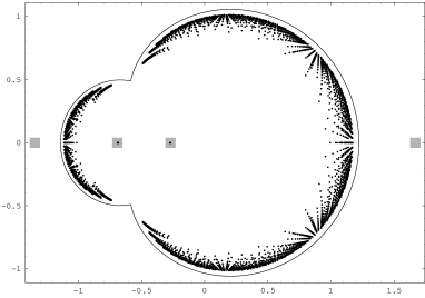
Figure 2: Zeros of $F_{n}(z)$, $n=\overline{20,90}$, for a $\psi$ as in (3.11) with $\omegaup=\exp(3\pi i/4)$.

If $\theta_{2}$ is irrational, then a point $t$ interior to $L$ is an accumulation point of the zeros of the $F_{n}$’s if and only if $t$ is real. In Figure 3 below, we have plotted the zeros of $F_{n}(z)$ for $n=\overline{20,90}$ corresponding to the case $\Theta_{1}=\sqrt{2}\pi/2$.

Figure 3: Zeros of $F_{n}(z)$, $n=\overline{20,90}$, for a $\psi$ as in (3.11) with $\omegaup=\exp(\sqrt{2}\pi i/2)$.

We finish this section presenting an example in which condition $A.3$ is not satisfied. Let $s\geq 2$ be a given integer. The function $w\mapsto w^{s}+1$ maps each of the $s$ sectors

$$2\pi(k-1)/s<\arg(w)<2\pi k/s,\quad k=1,2,\ldots,s,$$

conformally onto the complex plane cut along the ray $[0,+\infty)$, and by agreeing in that

$$2\pi(k-1)\leq\arg(w^{s}+1)<2\pi k\quad\mathrm{whenever}\quad 2\pi(k-1)/s\leq\arg(w)<2\pi k/s,$$

we see that

$$\psi(w)=(w^{s}+1)^{1/s}$$

maps the exterior of the unit circle conformally onto the exterior of the lemniscate of $s$ petals $L=\{z:|z^{s}-1|=1\}$ (see Figure 4 for $s=3$).

Here, $\Omega=\{z:|z^{s}-1|>1\}$, $G=\{z:|z^{s}-1|<1\}$, and the inverse of $\psi$ is $\phi(z)=(z^{s}-1)^{1/s}$. Moreover, it is easily seen that $\psi$ satisfies conditions $A.1$ and $A.2$ with

$$\omegaup_{k}=e^{i(2k-1)\pi/s},\quad z_{k}=0\,,\quad\lambda_{k}=1/s,\quad k=1,2,\ldots,s.$$

The Faber polynomial $F_{n}(z)$ is the polynomial part of the Laurent expansion at $\infty$ of $(z^{s}-1)^{n/s}$. Hence, for any two integers $m\geq 0$ and $l\in\{0,1,\ldots,s-1\}$,

$$F_{sm+l}(z)=\sum_{j=0}^{m}\left(-1\right)^{j}{m+l/s\choose j}z^{s(m-j)+l},$$ (3.13)

where ${a\choose b}$ stands for the generalized binomial coefficient $\Gamma(a+1)/\left[\Gamma(b+1)\Gamma(a-b+1)\right]$. In particular, $F_{sm}(z)=\left(z^{s}-1\right)^{m}$.

The important feature to note of this example is that the function $H_{n}(z)$ defined in (3.3) is identically zero for every $n\not=s-1\mod s$ (recall Remark 5.4). This example has been previously studied by Ullman [20] for $s=2$, and by He [10] for $s\geq 2$. Observe from (3.13) that $F_{sm+l}(z)$ has a zero of multiplicity $l$ at the origin. Ullman and He showed that all other zeros lie strictly in $G$ (see Figure 4 below).

Theorem 3.9 below shows that for every $l\in\{1,2,\ldots,s-1\}$, we can properly normalize the subsequence $\left\{F_{sm+l}\right\}_{m\geq 0}$ so as to make it converge locally uniformly on $G$ to a function that never vanishes on $G$. Hence, for every compact set $E\subset G$, there exists $N_{E}$ such that if $n\not=0\mod s$, and $n>N_{E}$, then $F_{n}$ has no zeros on $E$. As a consequence, $\nu_{n}\overset{*}{\longrightarrow}\mu_{L}$ as $n\to\infty$, $n\not=0\mod s$, where

$$\mu_{L}=\frac{|z|^{s-1}|dz|}{2\pi},\quad z\in L,$$

is the equilibrium measure of $L$. Observe how the distribution function of $\mu_{L}$ is in total agreement with the density pattern followed by the zeros in Figure 4.

However, the zeros of $F_{sm}$ are fixed, namely $e^{2\pi ik/s}$, $1\leq k\leq s$, each of multiplicity $m$ and contained in $G$, and so

$$\nu_{sm}\overset{*}{\longrightarrow}\frac{1}{s}\sum_{k=1}^{s}\delta_{e^{2\pi ik/s}}\quad\mathrm{as}\ m\to\infty.$$

Thus, Corollary 3.2 does not necessarily hold in the absence of condition A.3.

Figure 4: Zeros of $F_{100}(z)$ for the domain $\Omega=\{z:|z^{3}-1|>1\}$.

Theorem 3.9.

For every $l\in\{1,2,\ldots,s-1\}$,

$$(-1)^{m+1}{sm+l\choose l/s-1}^{-1}F_{sm+l}(z)=\frac{1}{s^{l/s}z^{s-l}}\left[1+r_{m}(z)\right]$$

where

$$r_{m}(z)=\frac{1}{m}\left[\frac{(s-1)(s-l)(2s-l)}{2s^{3}}-\frac{1}{sz^{s}}\right]+\mathcal{O}\left(m^{-(1+s)/s}\right)$$

locally uniformly in $|z^{s}-1|<1$ as $m\to\infty$.

More important than Theorem 3.9 is its proof, which illustrates an approach to obtaining asymptotics for $F_{n}$ in cases where A.3 is not satisfied.

4 Lehman expansion of $\psi$ near $\omegaup_{k}$

Let $\zeta$ be a small open circular arc of $\mathbb{T}_{1}$ centered at $\omegaup_{k}$ such that $\overline{\zeta}\cap\{\omegaup_{1},\ldots,\omegaup_{s}\}=\{\omegaup_{k}\}$. The set $\zeta\setminus\{\omegaup_{k}\}$ consists of two circular arcs, say $\zeta^{+}$, $\zeta^{-}$, and by our assumption A.1 on $L$, there exist simple analytic arcs $\mathcal{L}^{+}\supset\psi\left(\overline{\zeta^{+}}\right)$ and $\mathcal{L}^{-}\supset\psi\left(\overline{\zeta^{-}}\right)$ of which $z_{k}$ is an interior point. Hence the map $\psi$, originally defined on $\Delta_{1}$, can be continued by the Schwarz reflection principle for analytic arcs [3] across both $\zeta^{+}$ and $\zeta^{-}$. Since the images of $\mathcal{L}^{+}$ and $\mathcal{L}^{-}$ in such reflections are again simple analytic arcs containing $z_{k}$ as an interior point, by applying subsequent reflections we can continue $\psi$ near $\omegaup_{k}$ onto the entire logarithmic Riemann surface $\mathcal{S}_{\omegaup_{k}}$ with branch point at $\omegaup_{k}$.

Let the functions $(w-\omegaup_{k})^{l+j\lambda_{k}}$, $l\geq 0$, $j\geq 1$, and $\log(w-\omegaup_{k})$ be defined in $\mathcal{S}_{\omegaup_{k}}$. In what follows we abbreviate by putting $y=w-\omegaup_{k}$. Lehman [15, Thm. 1] proved that $\psi$ has the following asymptotic expansion: if $\lambda_{k}$ is irrational, then

$$\psi(w)=\psi(\omegaup_{k})+\sum_{l=0}^{\infty}\sum_{j=1}^{\infty}c^{k}_{lj0}y^{l+j\lambda_{k}},\quad c^{k}_{010}\not=0\,;$$ (4.1)

if $\lambda_{k}=p/q$ is a fraction reduced to lowest terms, then

$$\psi(w) = \psi(\omegaup_{k})+\sum_{l=0}^{\infty}\sum_{j=1}^{q}\sum_{m=0}^{\lfloor l/p\rfloor}c^{k}_{ljm}y^{l+j\lambda_{k}}(\log y)^{m},\quad c^{k}_{010}\not=0.$$ (4.2)

The terms in the above series are assumed to be arranged in an order such that a term of the form $y^{l+j\lambda_{k}}(\log y)^{m}$ precedes one of the form $y^{l^{\prime}+j^{\prime}\lambda_{k}}(\log y)^{m^{\prime}}$ if either $l+j\lambda_{k}<l^{\prime}+j^{\prime}\lambda_{k}$ or $l+j\lambda_{k}=l^{\prime}+j^{\prime}\lambda_{k}$ and $m>m^{\prime}$.

The precise meaning of these expansions is the following: if according to the order explained above, (4.1) and (4.2) are written in the form

$$\psi(w)=\psi(\omegaup_{k})+\sum_{n=1}^{\infty}\chi_{n}(y),$$

then for all $N\geq 1$,

$$\psi(w)-\psi(\omegaup_{k})-\sum_{n=1}^{N}\chi_{n}(y)=o\left(\chi_{N}(y)\right)$$

as $w\to\omegaup_{k}$ from any finite sector $\vartheta_{1}\leq\arg(w-\omegaup_{k})\leq\vartheta_{2}$ of $\mathcal{S}_{\omegaup_{k}}$.

We write in (4.1) $c^{k}_{lj0}$ instead of simply $c^{k}_{lj}$ when $\lambda_{k}$ is irrational, because this will allow us to express many of the relations that follow in one single statement without having to distinguish between $\lambda_{k}$ being irrational or rational.

The coefficients $c^{k}_{ljm}$ in (4.1) and (4.2) depend on the values assigned to the functions $(w-\omegaup_{k})^{l+j\lambda_{k}}$, $\log(w-\omegaup_{k})$ at a specified point of $\mathcal{S}_{\omegaup_{k}}$. We shall assume that the values of $\psi$ in $\Delta_{1}$ define $\psi$ in the sector $\Theta_{k}-\pi<\arg(w-\omegaup_{k})<\Theta_{k}+\pi$ of $\mathcal{S}_{\omegaup_{k}}$, and that for every $w$ in this sector,

$$(y)^{l+j\lambda_{k}}=|y|^{l+j\lambda_{k}}e^{i(l+j\lambda_{k})\arg(y)},\quad\log y=\log|y|+i\arg(y),\quad y=w-\omegaup_{k}.$$

A more detailed description of these expansions is split in two cases:

Case $0<\lambda_{k}<2$, $\lambda_{k}\not\in\{1,2\}$: As in Section 3, we put $A_{k}:=c^{k}_{010}\not=0$, and it follows from (4.1) and (4.2) that for $\upsilon>0$ sufficiently small, say

$$\upsilon<\left\{\begin{array}[]{cc}\min\{\lambda_{k},1-\lambda_{k}\},&\quad\mathrm{if}\ 0<\lambda_{k}<1,\\ 2-\lambda_{k}\,,&\quad\mathrm{if}\ 1<\lambda_{k}<2,\end{array}\right.$$

the following relations hold: if $0<\lambda_{k}<1$, then

$$\psi(w)=\psi(\omegaup_{k})+A_{k}y^{\lambda_{k}}+c^{k}_{020}y^{2\lambda_{k}}+o\left(y^{2\lambda_{k}+\upsilon}\right);$$ (4.3)

if $\lambda_{k}=1/2$,

$$\psi(w)=\psi(\omegaup_{k})+A_{k}y^{\lambda_{k}}+c^{k}_{020}y^{2\lambda_{k}}+c^{k}_{111}y^{1+\lambda_{k}}(\log y)+c^{k}_{110}y^{1+\lambda_{k}}+o\left(y^{3\lambda_{k}+\upsilon}\right);$$ (4.4)

if $1<\lambda_{k}<2$,

$$\psi(w)=\psi(\omegaup_{k})+A_{k}y^{\lambda_{k}}+c^{k}_{110}y^{1+\lambda_{k}}+c^{k}_{020}y^{2\lambda_{k}}+o\left(y^{2\lambda_{k}+\upsilon}\right)$$ (4.5)

(notice that if $1<\lambda_{k}=p/q<2$, then $p\geq 3$, $q\geq 2$, and no $\log$-terms correspond to $l=0,1,2$).

Case $\lambda_{k}\in\{1,2\}$: Here $p=\lambda_{k},\ q=1$. If $\omegaup_{k}$ is relevant, then there is a smallest integer $r_{k}\geq\lambda_{k}$ for which a $\log$-term of the form $y^{r_{k}+\lambda_{k}}(\log y)^{m_{k}}$, $1\leq m_{k}\leq\lfloor r_{k}/\lambda_{k}\rfloor$, occurs in the expansion of $\psi$ about $\omegaup_{k}$, so that in case $m_{k}\geq 2$,

$$\psi(w) = \psi(\omegaup_{k})+\sum_{l=0}^{r_{k}-1}c^{k}_{l10}y^{l+\lambda_{k}}+A_{k}y^{\Lambda_{k}}(\log y)^{m_{k}}+B_{k}y^{\Lambda_{k}}(\log y)^{m_{k}-1}$$ (4.9)

$$+C_{k}y^{\Lambda_{k}}(\log y)^{m_{k}-2}+\left\{\begin{array}[]{ll}\underset{\,}{\mathcal{O}\left(y^{\Lambda_{k}}(\log y)^{m_{k}-3}\right)},&\quad\mathrm{if}\ m_{k}\geq 3,\\ \mathcal{O}\left(y^{\Lambda_{k}+1/2}\right),&\quad\mathrm{if}\ m_{k}=2,\end{array}\right.$$

while if $m_{k}=1$, then

$$\psi(w) = \psi(\omegaup_{k})+\sum_{l=0}^{r_{k}-1}c^{k}_{l10}y^{l+\lambda_{k}}+A_{k}y^{\Lambda_{k}}(\log y)^{m_{k}}+B_{k}y^{\Lambda_{k}}(\log y)^{m_{k}-1}$$ (4.12)

$$+\widetilde{C}_{k}y^{\Lambda_{k}+1}(\log y)^{\lfloor(r_{k}+1)/\lambda_{k}\rfloor}+\widetilde{D}_{k}y^{\Lambda_{k}+1}(\log y)^{\lfloor(r_{k}+1)/\lambda_{k}\rfloor-1}$$

$$+\left\{\begin{array}[]{ll}\mathcal{O}\left(y^{\Lambda_{k}+1}(\log y)^{\lfloor(r_{k}+1)/\lambda_{k}\rfloor-2}\right),&\quad\mathrm{if}\ \lfloor(r_{k}+1)/\lambda_{k}\rfloor\geq 2,\\ \mathcal{O}\left(y^{\Lambda_{k}+3/2}\right),&\quad\mathrm{if}\ \lfloor(r_{k}+1)/\lambda_{k}\rfloor=1,\end{array}\right.$$

where

$$\Lambda_{k}:=r_{k}+\lambda_{k},\ \,A_{k}:=c^{k}_{r_{k}1m_{k}}\not=0,\ \,B_{k}:=c^{k}_{r_{k}1(m_{k}-1)},\ \,C_{k}:=c^{k}_{r_{k}1(m_{k}-2)},$$ (4.13)

$$\widetilde{C}_{k}:=c^{k}_{(r_{k}+1)1\lfloor(r_{k}+1)/\lambda_{k}\rfloor},\quad\widetilde{D}_{k}:=c^{k}_{(r_{k}+1)1\left(\lfloor(r_{k}+1)/\lambda_{k}\rfloor-1\right)}\,.$$ (4.14)

Thus, setting

$$Q_{k}(w):=z_{k}+\sum_{l=0}^{r_{k}-1}c^{k}_{l10}y^{l+\lambda_{k}}=z_{k}+\mathcal{O}\left(y^{\lambda_{k}}\right),$$ (4.15)

we have that if $m_{k}\geq 2$, then

$$\psi^{\prime}(w) = Q_{k}^{\prime}(w)+A_{k}\Lambda_{k}y^{\Lambda_{k}-1}(\log y)^{m_{k}}+\left(A_{k}m_{k}+B_{k}\Lambda_{k}\right)y^{\Lambda_{k}-1}(\log y)^{m_{k}-1}$$ (4.18)

$$+\left[B_{k}(m_{k}-1)+C_{k}\Lambda_{k}\right]y^{\Lambda_{k}-1}(\log y)^{m_{k}-2}+\left\{\begin{array}[]{ll}\mathcal{O}\left(y^{\Lambda_{k}-1}(\log y)^{m_{k}-3}\right),&\quad\mathrm{if}\ m_{k}\geq 3,\\ \mathcal{O}\left(y^{\Lambda_{k}-1/2}\right),&\quad\mathrm{if}\ m_{k}=2,\end{array}\right.$$

while if $m_{k}=1$, then

$$\psi^{\prime}(w) = Q_{k}^{\prime}(w)+A_{k}\Lambda_{k}y^{\Lambda_{k}-1}(\log y)^{m_{k}}+\left(A_{k}m_{k}+B_{k}\Lambda_{k}\right)y^{\Lambda_{k}-1}(\log y)^{m_{k}-1}$$ (4.22)

$$+\widetilde{C}_{k}\left(\Lambda_{k}+1\right)y^{\Lambda_{k}}(\log y)^{\lfloor(r_{k}+1)/\lambda_{k}\rfloor}$$

$$+\left[\widetilde{C}_{k}\lfloor(r_{k}+1)/\lambda_{k}\rfloor+\widetilde{D}_{k}\left(\Lambda_{k}+1\right)\right]y^{\Lambda_{k}}(\log y)^{\lfloor(r_{k}+1)/\lambda_{k}\rfloor-1}$$

$$+\left\{\begin{array}[]{ll}\mathcal{O}\left(y^{\Lambda_{k}+1/2}\right)&\quad\mathrm{if}\ \lfloor(r_{k}+1)/\lambda_{k}\rfloor=1,\\ \mathcal{O}\left(y^{\Lambda_{k}}(\log y)^{\lfloor(r_{k}+1)/\lambda_{k}\rfloor-2}\right)&\quad\mathrm{if}\ \lfloor(r_{k}+1)/\lambda_{k}\rfloor\geq 2\,.\end{array}\right.$$

If $\omegaup_{k}$ is not relevant, then for every $N\in\mathbb{N}$,

$$\psi(\omegaup_{k})=\psi(\omegaup_{k})+\sum_{l=0}^{N}c^{k}_{l10}y^{l+\lambda_{k}}+o\left(y^{N+\lambda_{k}}\right)=Q_{k}(z)+o\left(y^{N+\lambda_{k}}\right),$$ (4.23)

where

$$Q_{k}(z):=z_{k}+\sum_{l=0}^{N}c^{k}_{l10}y^{l+\lambda_{k}}.$$ (4.24)

The polynomial $Q_{k}(z)$ defined by (4.24) depends on the value $N$, so that in what follows we will think of $N$ as an arbitrarily large natural number that has been fixed.

5 Proofs of the asymptotic results

Recall we are using the notation

$$\mathbb{T}_{r}:=\{w:|w|=r\},\quad\mathbb{D}_{r}:=\{w:|w|<r\},\quad\Delta_{r}:=\{w:r<|w|\leq\infty\}.$$

Also, for $a,\,b\in\mathbb{C}$, we denote by $[a,b]$ the oriented closed segment that starts at $a$ and ends at $b$. A similar meaning is attached to $(a,b)$, $(a,b]$ and $[a,b)$. For every $0<\sigma<1$, we define

$$\sigma_{k}:=\sigma\omegaup_{k}\,,\qquad 1\leq k\leq s,$$

and the contour

$$\Gamma_{\sigma}:=\mathbb{T}_{\sigma}\cup\left(\cup_{k=1}^{s}[\sigma_{k},\omegaup_{k}]\right)\,.$$

The exterior of the contour $\Gamma_{\sigma}$, denoted by $\mathrm{ext}(\Gamma_{\sigma})$, is understood to be the unbounded component of $\overline{\mathbb{C}}\setminus\Gamma_{\sigma}$, that is,

$$\mathrm{ext}(\Gamma_{\sigma})=\Delta_{\sigma}\setminus\left(\cup_{k=1}^{s}[\sigma_{k},\omegaup_{k}]\right)\,.$$

Disregarding technical difficulties, the idea behind the proofs of the asymptotic results is simple, and in rough terms can be described as follows. By the piecewise analyticity of $\partial\Omega$, if $1-\sigma$ is small enough, the function $w^{n}\psi^{\prime}(w)/(\psi(w)-z)$ (in the variable $w$, for fixed $z$) has a meromorphic extension to $\mathrm{ext}(\Gamma_{\sigma})$ with at most finitely many poles in there and continuous boundary values on $\Gamma_{\sigma}$. Then, using the integral representation (1.3), we can express $F_{n}(z)$ as the sum of the residues of that function in $\mathrm{ext}(\Gamma_{\sigma})$, plus its integral (with respect to $w$) over $\Gamma_{\sigma}$, the later being split as an integral over $\mathbb{T}_{\sigma}$ (which is $\mathcal{O}(\sigma^{n})$ as $n\to\infty$, and therefore negligible) plus the integral of $w^{n}\psi^{\prime}(w)/(\psi(w)-z)$ over each of the “two-sided” segments $[\sigma_{k},\omegaup_{k}]$, $1\leq k\leq s$. The asymptotic behavior as $n\to\infty$ of these last integrals (as functions of $z$) can then be obtained from the Lehman expansions of $\psi$ about the $\omegaup_{k}$’s.

The first step in doing all this rigorously is to prove that a contour $\Gamma_{\sigma}$ satisfying the necessary conditions exists. That is the content of Lemmas 5.1 and 5.2 below.

For given $\delta>0$ and $t\in\mathbb{C}$, we put

$$D_{\delta}(t):=\{w:|w-t|<\delta\},\quad D_{\delta}^{*}(t):=\{w:0<|w-t|<\delta\}.$$

Then, for $\delta>0$ sufficiently small, the set

$$\zeta_{k,\delta}:=D_{\delta}(\omegaup_{k})\cap\mathbb{T}_{1}$$

is a circular arc, and $\zeta_{k,\delta}\setminus\{\omegaup_{k}\}$ is the union of two disjoint open circular arcs that we denote by $\zeta_{k,\delta}^{+}$, $\zeta_{k,\delta}^{-}$, say $\zeta_{k,\delta}^{-}$ immediately followed by $\zeta_{k,\delta}^{+}$ when $\mathbb{T}_{1}$ is traveled in counterclockwise direction.

Let

$$D^{+}_{\delta}(\omegaup_{k}):=D^{*}_{\delta}(\omegaup_{k})\setminus\zeta_{k,\delta}^{+},\quad D^{-}_{\delta}(\omegaup_{k}):=D^{*}_{\delta}(\omegaup_{k})\setminus\zeta_{k,\delta}^{-}\,.$$

If $\delta$ is sufficiently small, the disks $D_{\delta}(\omegaup_{1}),D_{\delta}(\omegaup_{2}),\dots,D_{\delta}(\omegaup_{s})$ are pairwise disjoint, and for every $k\in\{1,2,\ldots,s\}$, the mapping $\psi$ has analytic continuations $\psi_{+}$, $\psi_{-}$ from the exterior $\Delta_{1}$ of the unit circle to $D^{+}_{\delta}(\omegaup_{k})$, $D^{-}_{\delta}(\omegaup_{k})$, respectively.

Recall that $L_{1}$ and $L_{2}$ are defined by (2.7)-(2.8), and that for every $k$ with $\lambda_{k}\in\{1,2\}$, $Q_{k}$ is defined by (4.15) and (4.24).

Lemma 5.1.

Let $\epsilon>0$ be given. For every $\delta>0$ sufficiently small the following statements hold true:

1. For all $k\in\{1,2,\ldots,s\}$,

   $$\overline{\psi_{\pm}\left(D^{\pm}_{\delta}(\omegaup_{k})\right)}\subset D_{\epsilon}(z_{k})\,$$ (5.1)

   and

   $$\psi_{\pm}\left(w\right)\not=z_{k}\,,\quad\psi^{\prime}_{\pm}(w)\not=0\quad\forall\,w\in D^{\pm}_{\delta}(\omegaup_{k}).$$ (5.2)

   Also, for every $k$ with $\lambda_{k}\in\{1,2\}$, we have that

   $$Q_{k}(w)\not=z_{k}\quad\forall\,w\in D^{*}_{\delta}(\omegaup_{k}).$$ (5.3)

2. If $\tau_{k}:=(1-\delta)\omegaup_{k}$, there is a constant $C$ such that for every $k$ with $z_{k}\in L_{1}$ (resp. $z_{k}\in L_{2}$),

   $$\left|\frac{\psi_{\pm}(t)-z_{k}}{\psi_{\pm}(t)-z}\right|<C,\quad\left|\frac{Q_{k}(t)-z_{k}}{Q_{k}(t)-z}\right|<C,$$ (5.4)

   for all $t\in(\tau_{k},\omegaup_{k})$ and $z\in\overline{\Omega}$ (resp. $z\in L_{2}$).

Proof of Lemma 5.1.

Since for every $k\in\{1,2,\ldots,s\}$, $\psi$ has an analytic continuation to the entire logarithmic Riemann surface with branch point at $\omegaup_{k}$, and it is such that

$$\psi(w)-z_{k}=c^{k}_{010}(w-\omegaup_{k})^{\lambda_{k}}(1+o(1))\,,\quad c^{k}_{010}\not=0,$$ (5.5)

$$\psi^{\prime}(w)=c^{k}_{010}\lambda_{k}(w-\omegaup_{k})^{\lambda_{k}-1}(1+o(1))\,,$$ (5.6)

as $w\to\omegaup_{k}$ from any finite sector of the surface, and since by the very definition of $Q_{k}$ in (4.15) and (4.24), for every $k$ with $\lambda_{k}\in\{1,2\}$

$$Q_{k}(w)-z_{k}=c^{k}_{010}(w-\omegaup_{k})^{\lambda_{k}}(1+o(1)),$$ (5.7)

as $w\to\omegaup_{k}$, the conditions of part (a) of Lemma 5.1 will be trivially satisfied provided that $\delta$ is small enough.

Let us now prove part (b) of the lemma. The analysis is split in two cases.

Case 1: $k$ is such that $z_{k}\in L_{1}\cup L_{2}$ and $\lambda_{k}=1$. Under this assumption, there is a small open circular arc $\zeta_{k}\subset\mathbb{T}_{1}$, with center point $\omegaup_{k}$, such that $\psi$ is one-to-one on $\zeta_{k}$ and therefore $\psi(\zeta_{k})$ is a simple smooth arc containing $z_{k}$ as an interior point. We first verify the following

Claim: There is a small open disk $O_{k}$ centered at $z_{k}$ such that if $z_{k}\in L_{2}$, then $O_{k}\cap L_{2}\subset\psi(\zeta_{k})$, while if $z_{k}\in L_{1}$, then $O_{k}\cap L\subset\psi(\zeta_{k})$ and $O_{k}\setminus\psi(\zeta_{k})$ is the disjoint union of two nonempty connected open sets, one contained in $\Omega$, the other in $G$.

Let us prove the claim. Suppose $z_{k}\in L_{2}$ and let $t_{k}\not=\omegaup_{k}$ be the other point of $\mathbb{T}_{1}$ such that $\psi(t_{k})=z_{k}$. Then, there is also a small open circular arc $\rho_{k}\subset\mathbb{T}_{1}$, with center point $t_{k}$, such that $\psi$ is one-to-one on $\rho_{k}$. Since $\eta(z_{k})=2$, the closed set $\psi\left(\mathbb{T}_{1}\setminus(\zeta_{k}\cup\rho_{k})\right)$ cannot contain $z_{k}$, so that there is a small open disk $O_{k}$ centered at $z_{k}$ such that $\{t\in\mathbb{T}_{1}:\psi(t)\in O_{k}\}\subset(\zeta_{k}\cup\rho_{k})$. But since $\psi$ is one-to-one on $\rho_{k}$, we must have that $O_{k}\cap L_{2}\subset\psi(\zeta_{k})$. Similarly, suppose $z_{k}\in L_{1}$ and let $\delta^{\prime}>0$ be so small that the connected open set $\psi(D_{\delta^{\prime}}(\omegaup_{k})\cap\Delta_{1})$ lies strictly on one side of the arc $\psi(\zeta_{k})$. Since $\eta(z_{k})=1$, the closed set $\psi\left(\overline{\Delta}_{1}\setminus D_{\delta^{\prime}}(\omegaup_{k})\right)$ cannot contain $z_{k}$, and therefore, there is a sufficiently small open disk $O_{k}$ centered at $z_{k}$ such that $O_{k}\cap\psi\left(\overline{\Delta}_{1}\setminus D_{\delta^{\prime}}(\omegaup_{k})\right)=\emptyset$. In consequence, $O_{k}$ is divided by the arc $\psi(\zeta_{k})$ into two connected open sets, one contained in $\psi(D_{\delta^{\prime}}(\omegaup_{k})\cap\Delta_{1})\subset\Omega$, the other contained in $G$. The claim is proven.

Now, for every $k$ with $z_{k}\in L_{1}\cup L_{2}$, choose $O_{k}$ as in the claim, and assume $\delta>0$ is so small that, besides satisfying part (a) of the lemma, it also satisfies that $\overline{\psi_{\pm}\left(D^{\pm}_{\delta}(\omegaup_{k})\right)}\subset O_{k}$. By our assumption A.1 on $L$, there are two simple analytic arcs $\mathcal{L}_{k}^{+}$, $\mathcal{L}_{k}^{-}$, each containing $z_{k}$ as an interior point, and such that $\psi\left(\overline{\zeta_{k,\delta}^{+}}\right)\subset\mathcal{L}_{k}^{+}$, $\psi\left(\overline{\zeta_{k,\delta}^{-}}\right)\subset\mathcal{L}_{k}^{-}$. Notice that $\mathcal{L}^{\pm}_{k}$ and $\psi(\zeta_{k})$ share the same tangent line at $z_{k}$. In consequence, if $\tau_{k}:=(1-\delta)\omegaup_{k}$, the arc $\psi\left(\left(\omegaup_{k},1/\overline{\tau}_{k}\right)\right)$ lies entirely in $\Omega$, and by (5.5), it is perpendicular to $\psi(\zeta_{k})$.

By the Schwarz reflection principle for analytic arcs [3], if $\tau_{k}$ is close enough to $\omegaup_{k}$, $\psi_{\pm}((\tau_{k},\omegaup_{k}))$ is the reflection of $\psi\left(\left(\omegaup_{k},1/\overline{\tau}_{k}\right)\right)$ across $\mathcal{L}^{\mp}_{k}$, and therefore, for all $\delta$ sufficiently small, the arc $\psi_{\pm}((\tau_{k},\omegaup_{k}))$ is perpendicular to $\psi(\zeta_{k})$ and

$$\psi_{\pm}\left((\tau_{k},\omegaup_{k})\right)\subset G,\quad\psi\left(\mathbb{D}_{1}\cap D_{\delta}(\omegaup_{k})\setminus(\tau_{k},\omegaup_{k}]\right)\subset G\quad if\ z_{k}\in L_{1},$$ (5.8)

$$\psi_{\pm}\left((\tau_{k},\omegaup_{k})\right)\cap L_{2}=\emptyset,\quad\psi\left(\mathbb{D}_{1}\cap D_{\delta}(\omegaup_{k})\setminus(\tau_{k},\omegaup_{k}]\right)\cap L_{2}=\emptyset\quad if\ z_{k}\in L_{2},\ \lambda_{k}=1,$$ (5.9)

whence it follows at once that the first inequality of (5.4) holds true.

Similar considerations apply to $Q_{k}$. Because of (5.7), if $z_{k}\in L_{1}\cup L_{2}$ and $\lambda_{k}=1$, then $Q_{k}$ maps a small circular arc of $\mathbb{T}_{1}$ centered at $\omegaup_{k}$ onto an analytic arc tangent to $\psi(\zeta_{k})$ at $z_{k}$, and therefore, for all $\delta$ sufficiently small, $Q_{k}((\tau_{k},\omegaup_{k}))$ is perpendicular to $\psi(\zeta_{k})$ and is contained entirely in $G$, whence the second inequality of (5.4) follows.

Case 2: $k$ is such that $\lambda_{k}=2$. Let $\zeta_{k}\subset\mathbb{T}_{1}$ be a small open circular arc with center point at $\omegaup_{k}$, so that $\zeta_{k}\setminus\{\omegaup_{k}\}$ splits into two disjoint circular arcs $\zeta^{+}_{k}$ and $\zeta^{-}_{k}$. If $\zeta_{k}$ is small enough, $\psi\left(\overline{\zeta^{+}_{k}}\right)$ and $\psi\left(\overline{\zeta^{-}_{k}}\right)$ are simple analytic arcs forming a cusp pointing toward $\Omega$. Since $\lambda_{k}=2$ and all $\lambda_{j}$’s are strictly positive (that is, $\Omega$ has not outward pointing cusps), $\eta(z_{k})=1$ and there is an open disk $O_{k}$ centered a $z_{k}$ such that $O_{k}\cap L\subset\psi(\zeta_{k})$. But if two analytic arcs coincide at infinitely many points, they must be part of one and the same arc, so that if $O_{k}$ is sufficiently small, either $O_{k}\cap L_{2}=\{z_{k}\}$ or $z_{k}$ is the endpoint of a cut, that is, one of the two arcs $\psi\left(\overline{\zeta^{+}_{k}}\right)$, $\psi\left(\overline{\zeta^{-}_{k}}\right)$ is contained in the other.

Reasoning as we did for the case $\lambda_{k}=1$ above, we derive from the Schwarz reflection principle that for all $\delta$ sufficiently small, the arc $\psi_{\pm}((\tau_{k},\omegaup_{k}))$ forms angle $\pi$ with each of the arcs $\psi\left(\overline{\zeta^{+}_{k}}\right)$, $\psi\left(\overline{\zeta^{-}_{k}}\right)$ and

$$\psi_{\pm}\left((\tau_{k},\omegaup_{k})\right)\cap L_{2}=\emptyset,\quad\psi\left(\mathbb{D}_{1}\cap D_{\delta}(\omegaup_{k})\setminus(\tau_{k},\omegaup_{k}]\right)\cap L_{2}=\emptyset,$$ (5.10)

whence the first inequality of (5.4) easily follows.

Similarly, by (5.7), if $\lambda_{k}=2$, then for all $\delta$ sufficiently small, $Q_{k}((\tau_{k},\omegaup_{k}))$ forms angle $\pi$ with each of the arcs $\psi\left(\overline{\zeta^{+}_{k}}\right)$, $\psi\left(\overline{\zeta^{-}_{k}}\right)$, whence the second inequality of (5.4) follows.

∎

Lemma 5.2.

Let $E$ be a (fixed) closed set $(\infty\not\in E)$ such that either $E\subset G$, or $E\subset\Omega\cup L_{1}$ or $E\subset L_{2}$, or $E=\{z_{1},\ldots,z_{s}\}$. Then for all $\sigma<1$ with $1-\sigma$ sufficiently small, we have

1. $\psi$ has an analytic continuation to $\mathrm{ext}(\Gamma_{\sigma})$ with $\psi^{\prime}(w)\not=0$ for all $w\in\mathrm{ext}(\Gamma_{\sigma})$, and both $\psi$ and $\psi^{\prime}$ have continuous boundary values on $\Gamma_{\sigma}\setminus\{\omegaup_{1},\ldots\omegaup_{s}\}$ when viewing each $[\sigma_{k},\omegaup_{k}]$ as having two sides;

2. if $E\subset G$, then for every $z\in E$, $\psi^{\prime}(w)/(\psi(w)-z)$ is analytic on $\mathrm{ext}(\Gamma_{\sigma})$ with continuous boundary values on $\Gamma_{\sigma}\setminus\{\omegaup_{1},\ldots,\omegaup_{s}\}$;

3. if either $E\subset\Omega\cup L_{1}$, or $E\subset L_{2}$, or $E=\{z_{1},\ldots,z_{s}\}$, then for every $z\in E$, $\psi^{\prime}(w)/(\psi(w)-z)$ is analytic on

   $$\mathrm{ext}(\Gamma_{\sigma})\setminus\left\{\phi_{1}(z),\ldots,\phi_{\eta(z)}(z)\right\},$$

   with a simple pole at each $\phi_{j}(z)\not\in\{\omegaup_{1},\ldots,\omegaup_{s}\}$ and continuous boundary values on $\Gamma_{\sigma}\setminus\{\omegaup_{1},\ldots,\omegaup_{s}\}$ .

Proof of Lemma 5.2.

Part (a) and (b): Let $\delta>0$ be such that for every $k\in\{1,2,\ldots,s\}$, the analytic continuations $\psi_{\pm}$ of $\psi$ to $D^{\pm}_{\delta}(\omegaup_{k})$ satisfy that

$$\psi^{\prime}_{\pm}(w)\not=0\quad\forall\,w\in D^{\pm}_{\delta}(\omegaup_{k}).$$ (5.11)

Fix $\delta^{\prime}$ with $0<\delta^{\prime}<\delta$, and for every $\sigma$ with $1-\delta^{\prime}<\sigma<1$, consider the open set

$$A_{\delta^{\prime},\sigma}:=\left\{w:\sigma<|w|<1/\sigma,\ w\not\in\cup_{k=1}^{s}D_{\delta^{\prime}}(\omegaup_{k})\right\},$$

that consists of $s$ open components $A^{l}_{\delta^{\prime},\sigma}$, $l=1,2,\ldots,s$. Then, by assumption A.1 on $L$, the univalency of $\psi$ on $\Delta_{1}$, and the way analytic functions are continued across analytic arcs by means of the Schwarz reflection principle, we have that if $1-\sigma$ is small enough, then $\psi$ has an analytic and univalent continuation to each $A^{l}_{\delta^{\prime},\sigma}$. From this and (5.11), it follows that statement (a) holds for all $\Gamma_{\sigma}$ with $\sigma$ sufficiently close to $1$. Moreover, if $E\subset G$ and $\sigma$ is so close to $1$ that $\overline{\psi(\mathrm{ext}(\Gamma_{\sigma}))}\cap E=\emptyset$, then (b) obviously holds.

Part (c): Suppose first that either $E\subset\Omega\cup L_{1}$ or $E\subset L_{2}$. Let $\epsilon$ be such that

$$0<\epsilon<\mathrm{dist}\left(E,\left\{z_{k}:z_{k}\not\in E,\ 1\leq k\leq s\right\}\right)$$

For this $\epsilon$, choose $\delta>0$ for which (5.8), (5.9) and (5.10) hold true.

Let $E_{1}^{-1}:=\left\{w\in\mathbb{T}_{1}\setminus\cup_{k=1}^{s}D_{\delta}(\omegaup_{k}):\psi(w)\in E\right\}$. Then $E_{1}^{-1}$ is a compact set, and again, by the Schwarz reflection principle, we can find a finite set of open disks $U_{1},U_{2},\ldots,U_{m}$, each centered at some point of $E_{1}^{-1}$, such that $E_{1}^{-1}\subset\cup_{j=1}^{m}U_{j}$ and for all $1\leq j\leq m$, $\psi$ has an analytic and univalent continuation to each $U_{j}$, which satisfies

1. $\psi\left(\mathbb{D}_{1}\cap U_{j}\right)\subset G$, in case $E\subset\Omega\cup L_{1}$,

2. $\psi\left(U_{j}\setminus\mathbb{T}_{1}\right)\cap L_{2}=\emptyset$, in case $E\subset L_{2}$.

On the other hand, if $E=\{z_{1},\ldots,z_{s}\}$, choose $\epsilon>0$ such that

$$D_{\epsilon}(z_{k})\cap D_{\epsilon}(z_{j})=\emptyset\quad\mathrm{whenever}\quad z_{k}\not=z_{j},$$ (5.12)

and for this $\epsilon$ choose $\delta>0$ so that Lemma 5.1 holds. In this case,

$$E_{1}^{-1}:=\left\{w\in\mathbb{T}_{1}\setminus\cup_{k=1}^{s}D_{\delta}(\omegaup_{k}):\psi(w)\in E\right\}$$

has, say, $m\geq 0$ elements and we can find $m$ open disks $U_{1},U_{2},\ldots,U_{m}$, each centered at some $w\in E^{-1}_{1}$, such that for all $j\in\{1,\ldots,m\}$, $\psi$ has an analytic and univalent continuation to each $U_{j}$, which satisfies that

1. $\psi\left(U_{j}\setminus\mathbb{T}_{1}\right)\cap\{z_{1},\ldots,z_{s}\}=\emptyset$.

Now, in either of the three cases i), ii) and iii) above, the set

$$Y:=\mathbb{T}_{1}\setminus\left[\left(\cup_{k=1}^{s}D_{\delta}(\omegaup_{k})\right)\cup\left(\cup_{j=1}^{m}U_{j}\right)\right]$$

is compact, $\psi(Y)\cap E=\emptyset$, and therefore there is a neighborhood $W_{Y}$ of $Y$ such that the analytic continuation of $\psi$ to $W_{Y}$ satisfies

1. $\psi(W_{Y})\cap E=\emptyset$.

Then, part (c) holds for every $\sigma$ so close to 1 that

$$\left\{w:\sigma\leq|w|<1\right\}\subset W_{Y}\cup\left(\cup_{k=1}^{s}D_{\delta}(\omegaup_{k})\right)\cup\left(\cup_{j=1}^{m}U_{j}\right).$$

This follows for $E\subset\Omega\cup L_{1}$ from (5.8), i) and iv); for $E\subset L_{2}$ from (5.9)-(5.10), ii) and iv); and for $E=\{z_{1},\ldots,z_{s}\}$ from Lemma 5.1(a), (5.12), iii) and iv). ∎

Lemma 5.3.

Let $\epsilon>0$ and $\delta>0$ be such that $\overline{\psi_{\pm}\left(D^{\pm}_{\delta}(\omegaup_{k})\right)}\subset D_{\epsilon}(z_{k})$. Then, for every $\sigma$ with $0<1-\sigma<\delta$, we have that

1. if $\omegaup_{k}$ is relevant (that is, if $1\leq k\leq v$), then

   $$\frac{1}{2\pi i}\int_{\sigma_{k}}^{\omegaup_{k}}\left(\frac{t^{n}\psi_{+}^{\prime}(t)}{\psi_{+}(t)-z}-\frac{t^{n}\psi_{-}^{\prime}(t)}{\psi_{-}(t)-z}\right)dt=\alpha_{\Lambda_{k}-1,M_{k}}(n)\left(\frac{\mathcal{C}_{k}A_{k}e^{i(n+\Lambda_{k})\Theta_{k}}}{z-z_{k}}+r_{\sigma_{k},n}(z)\right)$$ (5.13)

   with $r_{\sigma_{k},n}(z)$ converging uniformly to zero on $\{z:|z-z_{k}|\geq\epsilon\}$ as $n\to\infty$, and

   $$\mathcal{C}_{k}:=\left\{\begin{array}[]{ll}[\Gamma(-\lambda_{k})\Gamma(\lambda_{k})]^{-1},&\quad if\ \lambda_{k}\not\in\{1,2\},\\ (-1)^{\Lambda_{k}-1}m_{k}\Lambda_{k},&\quad if\ \lambda_{k}\in\{1,2\};\end{array}\right.$$

2. if $\omegaup_{k}$ is not relevant, then for every $\tau>0$,

   $$\frac{1}{2\pi i}\int_{\sigma_{k}}^{\omegaup_{k}}\left(\frac{t^{n}\psi_{+}^{\prime}(t)}{\psi_{+}(t)-z}-\frac{t^{n}\psi_{-}^{\prime}(t)}{\psi_{-}(t)-z}\right)dt=\mathcal{O}\left(n^{-\tau}\right)$$

   uniformly on $\{z:|z-z_{k}|\geq\epsilon\}$ as $n\to\infty$.

Remark 5.4.

A more detailed version of (5.13) given by equalities (5.21), (5.22), (5.23), (5.31) and (5.32) in the proof of Lemma 5.3 provides asymptotic formulas for the functions $r_{\sigma_{k},n}(z)$ from which the following table follows.

if $k$ is such that rate of decay of $r_{\sigma_{k},n}(z)$ is rate is exact iff $0<\lambda_{k}<1,\ \lambda_{k}\not=1/2$ $\mathcal{O}\left(n^{-\lambda_{k}}\right)$ $2c^{k}_{020}(z-z_{k})+(A_{k})^{2}\not=0$ $\lambda_{k}=1/2$ $\mathcal{O}\left(n^{-1}\log n\right)$ $c^{k}_{111}\not=0$ $1<\lambda_{k}<2$ $\mathcal{O}\left(n^{-1}\right)$ $c^{k}_{110}\not=0$ $\lambda_{k}\in\{1,2\},\ m_{k}\geq 2$ $\mathcal{O}\left(1/\log n\right)$ $A_{k}m_{k}+\Lambda_{k}c^{k}_{r_{k}1(m_{k}-1)}+i\Theta_{k}m_{k}A_{k}\Lambda_{k}\not=0$ $\lambda_{k}\in\{1,2\},\ m_{k}=1$ $\mathcal{O}\left(n^{-1}(\log n)^{\lfloor(r_{k}+1)/\lambda_{k}\rfloor-1}\right)$ $c^{k}_{(r_{k}+1)1\lfloor(r_{k}+1)/\lambda_{k}\rfloor}\not=0$

Given $k\in\{1,2,\ldots,s\}$ satisfying one of the conditions listed in the first column of the table, an estimate on the rate of decay of $r_{\sigma_{k},n}(z)$ holding uniformly as $n\to\infty$ on any closed set $E\subset\{z:|z-z_{k}|\geq\epsilon\}$ is given in the second column. The rate is exact for given $k$ and $E$ if and only if the condition in the third column is satisfied by every $z\in E$.

Proof of Lemma 5.3.

Part (a): First, notice that for every integer $N\geq 1$, we have the identity

$$\frac{1}{\psi(w)-z}=\sum_{j=0}^{N-1}\frac{\left[z_{k}-\psi(w)\right]^{j}}{\left(z_{k}-z\right)^{j+1}}+\frac{\left[z_{k}-\psi(w)\right]^{N}}{\left(z_{k}-z\right)^{N}\left[\psi(w)-z\right]}.$$ (5.14)

Suppose first that $\lambda_{k}\not\not\in\{1,2\}$. Then, combining identity (5.14) corresponding to $N=2$ with (4.3) and (4.5), we obtain that uniformly on $\left\{z:|z-z_{k}|\geq\epsilon\right\}$ as $w\to\omegaup_{k}$ ($y=w-\omegaup_{k}\to 0$)

$$\frac{1}{\psi(w)-z}=\frac{1}{z_{k}-z}-\frac{A_{k}y^{\lambda_{k}}}{(z_{k}-z)^{2}}+\left\{\begin{array}[]{cc}\mathcal{O}\left(y^{2\lambda_{k}}\right),&0<\lambda_{k}<1,\\ \mathcal{O}\left(y^{\lambda_{k}+1}\right),&1<\lambda_{k}<2\,.\end{array}\right.$$ (5.15)

The asymptotic expansion of $\psi^{\prime}$ about $\omegaup_{k}$ is obtained from that of $\psi$ by termwise differentiation, so that from (4.3), (4.4) and (5.15) we see that if $0<\lambda_{k}<1$, then uniformly on $\left\{z:|z-z_{k}|\geq\epsilon\right\}$ as $w\to\omegaup_{k}$,

$$\frac{\psi^{\prime}(w)}{\psi(w)-z}=\frac{A_{k}\lambda_{k}y^{\lambda_{k}-1}}{z_{k}-z}+\frac{\lambda_{k}\left[2c^{k}_{020}(z_{k}-z)-A_{k}^{2}\right]y^{2\lambda_{k}-1}}{(z_{k}-z)^{2}}+\mathcal{O}\left(y^{2\lambda_{k}+\upsilon-1}\right),$$ (5.16)

and more specifically, for $\lambda_{k}=1/2$,

$$\frac{\psi^{\prime}(w)}{\psi(w)-z} = \frac{A_{k}\lambda_{k}y^{\lambda_{k}-1}}{z_{k}-z}+\frac{\lambda_{k}\left[2c^{k}_{020}(z_{k}-z)-A_{k}^{2}\right]y^{2\lambda_{k}-1}}{(z_{k}-z)^{2}}$$ (5.17)

$$+\frac{c^{k}_{111}(1+\lambda_{k})y^{\lambda_{k}}(\log y)}{z_{k}-z}+\mathcal{O}\left(y^{\lambda_{k}}\right).$$

Similarly, if $1<\lambda_{k}<2$, then uniformly on $\left\{z:|z-z_{k}|\geq\epsilon\right\}$ as $w\to\omegaup_{k}$

$$\frac{\psi^{\prime}(w)}{\psi(w)-z}=\frac{A_{k}\lambda_{k}y^{\lambda_{k}-1}}{z_{k}-z}+\frac{c^{k}_{110}(1+\lambda_{k})y^{\lambda_{k}}}{z_{k}-z}+\mathcal{O}\left(y^{2\lambda_{k}-1}\right).$$ (5.18)

For the analytic functions $(w-\omegaup_{k})^{\beta}$, $\log(w-\omegaup_{k})$ in $D_{\delta}(\omegaup_{k})\cap\Delta_{1}$ corresponding to the branch of the argument

$$\Theta_{k}-\pi<\arg(w-\omegaup_{k})<\Theta_{k}+\pi,\quad w\in\mathbb{C}\setminus\{t\omegaup_{k}:t\leq 1\},$$

let us denote by $(w-\omegaup_{k})^{\beta}_{\pm}$ and $\log_{\pm}(w-\omegaup_{k})$ their analytic continuations from $D_{\delta}(\omegaup_{k})\cap\Delta_{1}$ onto $D^{\pm}_{\delta}(\omegaup_{k})$, respectively. If $n,\,m\geq 0$ are integers and $\beta>-1$, then

$$\int_{\sigma_{k}}^{\omegaup_{k}}t^{n}(t-\omegaup_{k})_{\pm}^{\beta}(\log_{\pm}(t-\omegaup_{k}))^{m}dt$$ (5.19)

$$= \int_{0}^{\omegaup_{k}}t^{n}(t-\omegaup_{k})_{\pm}^{\beta}(\log_{\pm}(t-\omegaup_{k}))^{m}dt-\int_{0}^{\sigma_{k}}t^{n}(t-\omegaup_{k})_{\pm}^{\beta}(\log_{\pm}(t-\omegaup_{k}))^{m}dt$$

$$= e^{\mp i\beta\pi}e^{i(n+1+\beta)\Theta_{k}}\int_{0}^{1}x^{n}(1-x)^{\beta}\left[\log(1-x)+i(\Theta_{k}\mp\pi)\right]^{m}dx+\mathcal{O}(\sigma^{n})$$

$$= e^{\mp i\beta\pi}e^{i(n+1+\beta)\Theta_{k}}\sum_{l=0}^{m}{m\choose l}\alpha_{\beta,m-l}(n)(i(\Theta_{k}\mp\pi))^{l}+\mathcal{O}(\sigma^{n}),$$

and

$$\int_{\sigma_{k}}^{\omegaup_{k}}\mathcal{O}\left(t^{n}(t-\omegaup_{k})_{\pm}^{\beta}(\log_{\pm}(t-\omegaup_{k}))^{m}\right)dt = \mathcal{O}\left(\alpha_{\beta,m}(n)\right)\,.$$ (5.20)

Then, we get by combining (5.16), (5.19), (5.20), (2) and the well-known identity

$$\Gamma(1-z)\Gamma(z)=-z\Gamma(-z)\Gamma(z)=\pi/\sin(\pi z),$$

that if $0<\lambda_{k}<1$, $\lambda_{k}\not=1/2$, then

$$\frac{1}{2\pi i}\int_{\sigma_{k}}^{\omegaup_{k}}\left(\frac{t^{n}\psi_{+}^{\prime}(t)}{\psi_{+}(t)-z}-\frac{t^{n}\psi_{-}^{\prime}(t)}{\psi_{-}(t)-z}\right)dt$$ (5.21)

$$= \frac{A_{k}\lambda_{k}\sin(\lambda_{k}\pi)e^{i(n+\lambda_{k})\Theta_{k}}\alpha_{\lambda_{k}-1,0}(n)}{\pi(z_{k}-z)}+\mathcal{O}\left(\alpha_{2\lambda_{k}+\upsilon-1,0}(n)\right)$$

$$+\frac{\left[2c^{k}_{020}(z_{k}-z)-A_{k}^{2}\right]\lambda_{k}\sin(2\pi\lambda_{k})e^{i(n+2\lambda_{k})\Theta_{k}}\alpha_{2\lambda_{k}-1,0}(n)}{\pi(z_{k}-z)^{2}}\,,$$

$$= \frac{\alpha_{\lambda_{k}-1,0}(n)}{\Gamma(-\lambda_{k})\Gamma(\lambda_{k})}\left(\frac{A_{k}e^{i(n+\lambda_{k})\Theta_{k}}}{z-z_{k}}\right.+o\left(n^{-\lambda_{k}}\right)$$

$$\left.\hskip 85.35826pt+\frac{\Gamma(-\lambda_{k})\left[2c^{k}_{020}(z-z_{k})+(A_{k})^{2}\right]e^{i(n+2\lambda_{k})\Theta_{k}}}{2\Gamma(-2\lambda_{k})(z-z_{k})^{2}n^{\lambda_{k}}}\right).$$

Similarly, we get from (5.17), that if $\lambda_{k}=1/2$, then

$$\frac{1}{2\pi i}\int_{\sigma_{k}}^{\omegaup_{k}}\left(\frac{t^{n}\psi_{+}^{\prime}(t)}{\psi_{+}(t)-z}-\frac{t^{n}\psi_{-}^{\prime}(t)}{\psi_{-}(t)-z}\right)dt$$ (5.22)

$$= \frac{\alpha_{\lambda_{k}-1,0}(n)}{\Gamma(-\lambda_{k})\Gamma(\lambda_{k})}\left(\frac{A_{k}e^{i(n+\lambda_{k})\Theta_{k}}}{z-z_{k}}+\frac{c^{k}_{111}(1+\lambda_{k})e^{i(n+\lambda_{k}+1)\Theta_{k}}(\log n)}{(z-z_{k})n}+o\left(n^{-1}\log n\right)\right),$$

and from (5.18) that if $1<\lambda_{k}<2$, then

$$\frac{1}{2\pi i}\int_{\sigma_{k}}^{\omegaup_{k}}\left(\frac{t^{n}\psi_{+}^{\prime}(t)}{\psi_{+}(t)-z}-\frac{t^{n}\psi_{-}^{\prime}(t)}{\psi_{-}(t)-z}\right)dt$$ (5.23)

$$= \frac{\alpha_{\lambda_{k}-1,0}(n)}{\Gamma(-\lambda_{k})\Gamma(\lambda_{k})}\left(\frac{A_{k}e^{i(n+\lambda_{k})\Theta_{k}}}{z-z_{k}}-\frac{c^{k}_{110}(1+\lambda_{k})e^{i(n+\lambda_{k}+1)\Theta_{k}}}{(z-z_{k})n}+o\left(n^{-1}\right)\right).$$

Thus, Lemma 5.3 for a relevant $\omegaup_{k}$ with $\lambda_{k}\not\in\{1,2\}$ follows from (5.21), (5.22) and (5.23).

Next, let us consider the case $\lambda_{k}\in\{1,2\}$. From (4.9) and (4.18) we see that if $m_{k}\geq 2$, then uniformly on $\{z:|z-z_{k}|\geq\epsilon\}$ as $w\to\omegaup_{k}$,

$$\frac{\psi^{\prime}(w)}{\psi(w)-z} = \frac{Q_{k}^{\prime}(w)}{Q_{k}(w)-z}+\frac{\psi^{\prime}(w)-Q_{k}^{\prime}(w)}{Q_{k}(w)-z}+\mathcal{O}\left(y^{\Lambda_{k}+\lambda_{k}-1}(\log y)^{m_{k}}\right)$$ (5.26)

$$= \frac{Q_{k}^{\prime}(w)}{Q_{k}(w)-z}+\left[\psi^{\prime}(w)-Q_{k}^{\prime}(w)\right]\left(\frac{1}{z_{k}-z}+\frac{z_{k}-Q_{k}(w)}{(z_{k}-z)(Q_{k}(w)-z)}\right)$$

$$+\mathcal{O}\left(y^{\Lambda_{k}+\lambda_{k}-1}(\log y)^{m_{k}}\right)$$

$$= \frac{Q_{k}^{\prime}(w)}{Q_{k}(w)-z}+\frac{A_{k}\Lambda_{k}y^{\Lambda_{k}-1}(\log y)^{m_{k}}}{z_{k}-z}+\frac{\left(A_{k}m_{k}+B_{k}\Lambda_{k}\right)y^{\Lambda_{k}-1}(\log y)^{m_{k}-1}}{z_{k}-z}$$

$$+\frac{\left[B_{k}(m_{k}-1)+C_{k}\Lambda_{k}\right]y^{\Lambda_{k}-1}(\log y)^{m_{k}-2}}{z_{k}-z}$$

$$+\left\{\begin{array}[]{ll}\mathcal{O}\left(y^{\Lambda_{k}-1}(\log y)^{m_{k}-3}\right)&\quad\mathrm{if}\ m_{k}\geq 3,\\ \mathcal{O}\left(y^{\Lambda_{k}-1/2}\right)&\quad\mathrm{if}\ m_{k}=2.\end{array}\right.$$

Similarly, one gets from (4.12) and (4.22) that if $m_{k}=1$ and $\lambda_{k}=2$, then

$$\frac{\psi^{\prime}(w)}{\psi(w)-z} = \frac{Q_{k}^{\prime}(w)}{Q_{k}(w)-z}+\frac{A_{k}\Lambda_{k}y^{\Lambda_{k}-1}(\log y)^{m_{k}}}{z_{k}-z}+\frac{\left(A_{k}m_{k}+B_{k}\Lambda_{k}\right)y^{\Lambda_{k}-1}(\log y)^{m_{k}-1}}{z_{k}-z}$$ (5.29)

$$+\frac{\widetilde{C}_{k}\left(\Lambda_{k}+1\right)y^{\Lambda_{k}}(\log y)^{\lfloor(r_{k}+1)/\lambda_{k}\rfloor}}{z_{k}-z}$$

$$+\frac{\left[\widetilde{C}_{k}\lfloor(r_{k}+1)/\lambda_{k}\rfloor+\widetilde{D}_{k}\left(\Lambda_{k}+1\right)\right]y^{\Lambda_{k}}(\log y)^{\lfloor(r_{k}+1)/\lambda_{k}\rfloor-1}}{z_{k}-z}$$

$$+\left\{\begin{array}[]{ll}\mathcal{O}\left(y^{\Lambda_{k}+1/2}\right)&\quad\mathrm{if}\ r_{k}=2,\\ \mathcal{O}\left(y^{\Lambda_{k}}(\log y)^{\lfloor(r_{k}+1)/\lambda_{k}\rfloor-2}\right)&\quad\mathrm{if}\ r_{k}\geq 3,\end{array}\right.$$

while if $m_{k}=1$ and $\lambda_{k}=1$, then uniformly on $\{z:|z-z_{k}|\geq\epsilon\}$ as $w\to\omegaup_{k}$,

$$\frac{1}{\psi(w)-z} = \frac{1}{Q_{k}(w)-z}+\frac{Q_{k}(w)-\psi(w)}{\left[Q_{k}(w)-z\right]^{2}}+\frac{\left[Q_{k}(w)-\psi(w)\right]^{2}}{\left[Q_{k}(w)-z\right]^{2}\left[\psi(w)-z\right]}$$

$$= \frac{1}{Q_{k}(w)-z}+\frac{Q_{k}(w)-\psi(w)}{\left(z_{k}-z\right)^{2}}+\mathcal{O}\left(y^{\Lambda_{k}}\right),$$

and so

$$\frac{\psi^{\prime}(w)}{\psi(w)-z} = \frac{Q_{k}^{\prime}(w)}{Q_{k}(w)-z}+\left[\psi^{\prime}(w)-Q_{k}^{\prime}(w)\right]\left(\frac{1}{z_{k}-z}+\frac{z_{k}-Q_{k}(w)}{(z_{k}-z)^{2}}\right)$$ (5.30)

$$-\frac{c^{k}_{010}A_{k}y^{\Lambda_{k}}(\log y)}{\left(z_{k}-z\right)^{2}}+\mathcal{O}\left(y^{\Lambda_{k}}\right)$$

$$= \frac{Q_{k}^{\prime}(w)}{Q_{k}(w)-z}+\frac{A_{k}\Lambda_{k}y^{\Lambda_{k}-1}(\log y)}{z_{k}-z}+\frac{\left(A_{k}+B_{k}\Lambda_{k}\right)y^{\Lambda_{k}-1}}{z_{k}-z}$$

$$+\frac{\widetilde{C}_{k}(\Lambda_{k}+1)y^{\Lambda_{k}}(\log y)^{r_{k}+1}}{z_{k}-z}$$

$$+\frac{\left[\widetilde{C}_{k}(r_{k}+1)+\widetilde{D}_{k}(\Lambda_{k}+1)\right]y^{\Lambda_{k}}(\log y)^{r_{k}}}{z_{k}-z}$$

$$-\frac{c^{k}_{010}A_{k}\Lambda_{k}y^{\Lambda_{k}}(\log y)}{z_{k}-z}-\frac{c^{k}_{010}A_{k}y^{\Lambda_{k}}(\log y)}{\left(z_{k}-z\right)^{2}}+\mathcal{O}\left(y^{\Lambda_{k}}(\log y)^{r_{k}-1}\right).$$

Thus, we get from (5.26), (5.29), (5.30), (5.19) and (5.20) that if $\lambda_{k}\in\{1,2\}$ and $m_{k}\geq 2$, then uniformly on $\{z:|z-z_{k}|\geq\epsilon\}$ as $w\to\omegaup_{k}$

$$\frac{1}{2\pi i}\int_{\sigma_{k}}^{\omegaup_{k}}\left(\frac{t^{n}\psi_{+}^{\prime}(t)}{\psi_{+}(t)-z}-\frac{t^{n}\psi_{-}^{\prime}(t)}{\psi_{-}(t)-z}\right)dt$$ (5.31)

$$= \frac{m_{k}\Lambda_{k}\alpha_{\Lambda_{k}-1,m_{k}-1}(n)}{(-1)^{\Lambda_{k}-1}}\left\{\frac{A_{k}e^{i(n+\Lambda_{k})\Theta_{k}}}{z-z_{k}}\right.+o\left(1/\log n\right)$$

$$\hskip 102.43008pt-\left.\frac{(m_{k}-1)\left(A_{k}m_{k}+B_{k}\Lambda_{k}+i\Theta_{k}m_{k}\Lambda_{k}A_{k}\right)e^{i(n+\Lambda_{k})\Theta_{k}}}{m_{k}\Lambda_{k}(z-z_{k})(\log n)}\right\},$$

while if $\lambda_{k}\in\{1,2\}$ and $m_{k}=1$, then uniformly on $\{z:|z-z_{k}|\geq\epsilon\}$ as $w\to\omegaup_{k}$

$$\frac{1}{2\pi i}\int_{\sigma_{k}}^{\omegaup_{k}}\left(\frac{t^{n}\psi_{+}^{\prime}(t)}{\psi_{+}(t)-z}-\frac{t^{n}\psi_{-}^{\prime}(t)}{\psi_{-}(t)-z}\right)dt$$ (5.32)

$$= \frac{m_{k}\Lambda_{k}\alpha_{\Lambda_{k}-1,m_{k}-1}(n)}{(-1)^{\Lambda_{k}-1}}\left\{\frac{A_{k}e^{i(n+\Lambda_{k})\Theta_{k}}}{z-z_{k}}\right.+o\left(n^{-1}(\log n)^{\lfloor(r_{k}+1)/\lambda_{k}\rfloor-1}\right)$$

$$\hskip 99.58464pt-\left.\frac{\lfloor(r_{k}+1)/\lambda_{k}\rfloor\Gamma(\Lambda_{k})\widetilde{C}_{k}(\Lambda_{k}+1)e^{i(n+\Lambda_{k}+1)\Theta_{k}}}{m_{k}\Lambda_{k}(z-z_{k})n(-\log n)^{1-\lfloor(r_{k}+1)/\lambda_{k}\rfloor}}\right\}.$$

This completes the proof of part (a) of Lemma 5.3. The proof of part (b) easily follows from (4.24) by proceeding similarly as in the proof of part (a). ∎

Proof of Theorem 2.1.

Let $E\subset G$ be a compact set, and let $0<\epsilon<\mathrm{dist}(E,\{z_{1},\ldots,z_{s}\})$. For this $\epsilon$, choose $\delta$ such that (5.1) holds, and fix $\sigma$ with $0<1-\sigma<\delta$ and satisfying Lemma 5.2(b).

By (1.3), if $R>1$, then

$$F_{n}(z)=\frac{1}{2\pi i}\varointctrclockwise_{\mathbb{T}_{R}}\frac{t^{n}\psi^{\prime}(t)dt}{\psi(t)-z}\quad\forall\,z\in E.$$ (5.33)

Since $\psi^{\prime}(w)/(\psi(w)-z)$ is analytic on $\mathrm{ext}(\Gamma_{\sigma})$ with continuous boundary values on $\Gamma_{\sigma}\setminus\{\omegaup_{1},\ldots,\omegaup_{s}\}$, and since by (4.1) and (4.2), for $k=1,2,\ldots,s$, $\psi^{\prime}(w)=\mathcal{O}\left((w-\omegaup_{k})^{\lambda_{k}-1}\right)$ as $w\to\omegaup_{k}$, then

$$\varointctrclockwise_{\mathbb{T}_{R}}\frac{t^{n}\psi^{\prime}(t)dt}{\psi(t)-z}=\varointctrclockwise_{\mathbb{T}_{\sigma}}\frac{t^{n}\psi^{\prime}(t)dt}{\psi(t)-z}+\sum_{k=1}^{s}\int_{\sigma_{k}}^{\omegaup_{k}}\left(\frac{t^{n}\psi_{+}^{\prime}(t)}{\psi_{+}(t)-z}-\frac{t^{n}\psi_{-}^{\prime}(t)}{\psi_{-}(t)-z}\right)dt,$$ (5.34)

so that by Lemma 5.3,

$$F_{n}(z) = \mathcal{O}\left(\sigma^{n}\right)+\sum_{k=1}^{s}\frac{1}{2\pi i}\int_{\sigma_{k}}^{\omegaup_{k}}\left(\frac{t^{n}\psi_{+}^{\prime}(t)}{\psi_{+}(t)-z}-\frac{t^{n}\psi_{-}^{\prime}(t)}{\psi_{-}(t)-z}\right)dt$$ (5.35)

$$= \alpha_{\Lambda_{1}-1,M_{1}}(n)\left(\mathcal{C}_{1}\sum_{k=1}^{u}\frac{A_{k}e^{i(n+\Lambda_{k})\Theta_{k}}}{z-z_{k}}+R_{n}(z)\right),$$

where (for every $\tau>0$),

$$R_{n}(z)=\sum_{k=1}^{u}r_{\sigma_{k},n}(z)+\sum_{k=u+1}^{v}\mathcal{O}\left(n^{\Lambda_{1}-\Lambda_{k}}(\log n)^{M_{k}-M_{1}}\right)+\mathcal{O}\left(n^{-\tau}\right)$$ (5.36)

uniformly in $z\in E$ as $n\to\infty$. Theorem 2.1 is proven. ∎

Proof of Theorem 2.3.

First, observe that it suffices to prove Theorem 2.3(a) assuming that $E$ does not contain $\infty$, because by the very definition of the Faber polynomials, $F_{n}(z)-[\phi(z)]^{n}$ is analytic at $\infty$, and an application of the maximum principle for analytic functions will extend the validity of the theorem to closed sets of $\Omega\cup L_{1}$ containing $\infty$.

Then, let $E$ be a closed set ($\infty\not\in E$) such that either $E\subset\Omega\cup L_{1}$ or $E\subset L_{2}$, and let

$$0<\epsilon<\mathrm{dist}\left(E,\left\{z_{k}:z_{k}\not\in E\right\}\right).$$

For this $\epsilon$, choose $\delta$ such that Lemma 5.1 holds, and fix $\sigma$ with $0<1-\sigma<\delta$ such that Lemma 5.2(c) holds.

Recall that $\eta(z)=1$ if $z\in\Omega\cup L_{1}$, $\eta(z)=2$ if $z\in L_{2}\setminus\{z_{k}:\lambda_{k}=2\}$, and that $\phi_{1}(z):=\phi(z)$ for all $z\in\Omega$.

For every $z\in E\setminus\{z_{1},\ldots,z_{s}\}$, $\phi_{l}(z)\in\mathrm{ext}(\Gamma_{\sigma})$, $l\in\{1,2,\ldots,\eta(z)\}$, and by Lemma 5.2(c), the function $w^{n}\psi^{\prime}(w)/\left[\psi(w)-z\right]$ is analytic in the variable $w$ on $\mathrm{ext}(\Gamma_{\sigma})\setminus\left\{\phi_{l}(z):1\leq l\leq\eta(z)\right\}$, with residue $[\phi_{l}(z)]^{n}$ at each (simple pole) $\phi_{l}(z)$ and continuous boundary values on $\Gamma_{\sigma}\setminus\{\omegaup_{1},\ldots,\omegaup_{s}\}$. Moreover, by (4.1) and (4.2), for $k=1,2,\ldots,s$, $\psi^{\prime}(w)=\mathcal{O}\left((w-\omegaup_{k})^{\lambda_{k}-1}\right)$ as $w\to\omegaup_{k}$, so that (1.3) and the residue theorem yield that for every $z\in E\setminus\{z_{1},\ldots,z_{s}\}$,

$$F_{n}(z)=\sum_{l=1}^{\eta(z)}[\phi_{l}(z)]^{n}+\frac{1}{2\pi i}\varointctrclockwise_{\mathbb{T}_{\sigma}}\frac{t^{n}\psi^{\prime}(t)dt}{\psi(t)-z}+\sum_{k=1}^{s}\frac{1}{2\pi i}\int_{\sigma_{k}}^{\omegaup_{k}}\left(\frac{t^{n}\psi_{+}^{\prime}(t)}{\psi_{+}(t)-z}-\frac{t^{n}\psi_{-}^{\prime}(t)}{\psi_{-}(t)-z}\right)dt.$$ (5.37)

In fact, we claim that for every $z\in E$,

$$F_{n}(z) = \Phi_{n}(z)+\frac{1}{2\pi i}\varointctrclockwise_{\mathbb{T}_{\sigma}}\frac{t^{n}\psi^{\prime}(t)dt}{\psi(t)-z}+\sum_{k\,:\,z_{k}\not\in E}\int_{\sigma_{k}}^{\omegaup_{k}}\left(\frac{t^{n}\psi_{+}^{\prime}(t)}{\psi_{+}(t)-z}-\frac{t^{n}\psi_{-}^{\prime}(t)}{\psi_{-}(t)-z}\right)dt$$ (5.38)

$$+\sum_{k\,:\,z_{k}\in E}\left(\varointctrclockwise_{[\sigma_{k},\omegaup_{k}]}\frac{t^{n}[\psi^{\prime}(t)-Q^{\prime}_{k}(t)]dt}{Q_{k}(t)-z}-\varointctrclockwise_{[\sigma_{k},\omegaup_{k}]}\frac{t^{n}[\psi(t)-Q_{k}(t)]\psi^{\prime}(t)dt}{\left(Q_{k}(t)-z\right)^{2}}\right.$$

$$\hskip 56.9055pt\left.+\varointctrclockwise_{[\sigma_{k},\omegaup_{k}]}\frac{t^{n}[\psi(t)-Q_{k}(t)]^{2}\psi^{\prime}(t)dt}{\left(Q_{k}(t)-z\right)^{2}(\psi(t)-z)}\right).$$

Indeed, for $z\in E\setminus\{z_{1},\ldots,z_{s}\}$, the claim is a direct consequence of (5.37) and the identity

$$\frac{\psi^{\prime}(w)}{\psi(w)-z} = \frac{Q_{k}^{\prime}(w)}{Q_{k}(w)-z}+\frac{\psi^{\prime}(w)-Q^{\prime}_{k}(w)}{Q_{k}(w)-z}-\frac{[\psi(w)-Q_{k}(w)]\psi^{\prime}(w)}{\left(Q_{k}(w)-z\right)^{2}}$$ (5.39)

$$+\frac{[\psi(w)-Q_{k}(w)]^{2}\psi^{\prime}(w)}{\left(Q_{k}(w)-z\right)^{2}(\psi(w)-z)},$$

taking into account that, by (5.3) and (5.4), $Q_{k}(w)-z\not=0$ for all $w\in[\sigma_{k},\omegaup_{k})$, $z\in\overline{\Omega}$

Suppose now $j$ is such that $z_{j}\in E$, and let us agree in that, in case $\eta(z_{j})=2$ and one of the two values $\phi_{1}(z_{j}),\phi_{2}(z_{j})$ is not contained in $\{\omegaup_{1},\ldots,\omegaup_{s}\}$, that value is precisely $\phi_{1}(z_{j})$.

Then, for every $k$ with $z_{k}=\psi(\omegaup_{k})=z_{j}$ (there are at most two of them), let $T_{k}\subset D_{\delta}(\omegaup_{k})$ be the circle centered at $\omegaup_{k}$ of radius $1-\sigma$. We can assume $\sigma$ was chosen so close to 1 that in case $z_{j}\in L_{2}$ and $\phi_{1}(z_{j})\not\in\{\omegaup_{1},\ldots,\omegaup_{s}\}$, $\phi_{1}(z_{j})$ lies in the exterior of $T_{k}$.

Then, we obtain once again from (1.3) and Lemma 5.2(c) that

$$F_{n}(z_{j}) = \frac{1}{2\pi i}\varointctrclockwise_{\mathbb{T}_{\sigma}}\frac{t^{n}\psi^{\prime}(t)dt}{\psi(t)-z_{j}}+\sum_{k\,:\,z_{k}\not=z_{j}}\frac{1}{2\pi i}\int_{\sigma_{k}}^{\omegaup_{k}}\left(\frac{t^{n}\psi_{+}^{\prime}(t)}{\psi_{+}(t)-z_{j}}-\frac{t^{n}\psi_{-}^{\prime}(t)}{\psi_{-}(t)-z_{j}}\right)dt$$ (5.42)

$$+\sum_{k\,:\,z_{k}=z_{j}}\frac{1}{2\pi i}\varointctrclockwise_{T_{k}}\frac{t^{n}\psi^{\prime}(t)dt}{\psi(t)-z_{k}}+\left\{\begin{array}[]{ll}[\phi_{1}(z_{j})]^{n},&\ \mathrm{if}\ \eta(z_{j})=2,\ \phi_{1}(z_{j})\not\in\{\omegaup_{1},\ldots,\omegaup_{s}\},\\ 0,&\ \mathrm{otherwise}.\end{array}\right.$$

By Lemma 5.1(a), $w^{n}Q^{\prime}_{k}(w)/\left(Q_{k}(w)-z_{k}\right)$ is analytic on $D^{*}_{\delta}(\omegaup_{k})$ with a simple pole at $\omegaup_{k}$, so that if we take identity (5.39) for $z=z_{k}$, multiply it by $w^{n}$ and integrating it over $T_{k}$, we obtain that for $k$ with $z_{k}=z_{j}$,

$$\varointctrclockwise_{T_{k}}\frac{t^{n}\psi^{\prime}(t)dt}{\psi(t)-z_{j}} = 2\pi i\lambda_{k}(\omegaup_{k})^{n}+\varointctrclockwise_{[\sigma_{k},\omegaup_{k}]}\frac{t^{n}[\psi^{\prime}(t)-Q^{\prime}_{k}(t)]dt}{Q_{k}(t)-z_{j}}-\varointctrclockwise_{[\sigma_{k},\omegaup_{k}]}\frac{t^{n}[\psi(t)-Q_{k}(t)]\psi^{\prime}(t)dt}{\left(Q_{k}(t)-z_{j}\right)^{2}}$$ (5.44)

$$+\varointctrclockwise_{[\sigma_{k},\omegaup_{k}]}\frac{t^{n}[\psi(t)-Q_{k}(t)]^{2}\psi^{\prime}(t)dt}{\left(Q_{k}(t)-z_{j}\right)^{2}(\psi(t)-z_{j})}\,.$$

Then, (5.38) for $z=z_{j}$ follows from relations (5.42) and (5.44).

Now that the claim is proven, we proceed to estimate the integrals that occur in (5.38) under the symbol $\sum_{k\,:\,z_{k}\in E}$ . For this, we first observe that if $\{\mathcal{F}(\cdot,z):z\in E\}$ is a uniformly bounded family of measurable functions on $[\sigma_{k},\omegaup_{k})$, if $n,\,m\geq 0$ are integers and $\beta>-1$, then (compare to (5.19))

$$\int_{\sigma_{k}}^{\omegaup_{k}}\mathcal{F}(t,z)t^{n}(t-\omegaup_{k})_{\pm}^{\beta}(\log_{\pm}(t-\omegaup_{k}))^{m}dt$$ (5.45)

$$= e^{\mp i\beta\pi}e^{i(n+1+\beta)\Theta_{k}}\sum_{l=0}^{m}{m\choose l}(i(\Theta_{k}\mp\pi))^{l}\alpha_{\beta,m-l}(n)G_{\beta,l,n}(z)+\mathcal{O}(\sigma^{n}),$$

where the functions

$$G_{\beta,l,n}(z):=\frac{\int_{0}^{1}\widetilde{\mathcal{F}}(x,z)x^{n}(1-x)^{\beta}(\log(1-x))^{m-l}dx}{\alpha_{\beta,m-l}(n)},\quad\widetilde{\mathcal{F}}(x,z):=\left\{\begin{array}[]{ll}\mathcal{F}\left(xe^{i\Theta_{k}},z\right),&\ x\in[\sigma,1),\\ 1,&\ x\in[0,\sigma),\end{array}\right.$$

are uniformly bounded on $E$, are independent of the sign $\pm$, and $G_{\beta,l,n}(z)=1$ whenever $\mathcal{F}(\cdot,z)\equiv 1$.

Now, assume $\omegaup_{k}$ is relevant. Recall that with $y=w-\omegaup_{k}$ (see (4.15), (4.12), (4.18) and (4.22)),

$$Q_{k}(w)=z_{k}+c^{k}_{010}y^{\lambda_{k}}+\mathcal{O}\left(y^{\lambda_{k}+1}\right),\quad Q_{k}^{\prime}(w)=c^{k}_{010}\lambda_{k}y^{\lambda_{k}-1}+\mathcal{O}\left(y^{\lambda_{k}}\right),$$ (5.46)

$$\psi(w)-Q_{k}(w) = A_{k}y^{\Lambda_{k}}(\log y)^{m_{k}}+B_{k}y^{\Lambda_{k}}(\log y)^{m_{k}-1}$$ (5.49)

$$+\left\{\begin{array}[]{cc}\mathcal{O}\left(y^{\Lambda_{k}}(\log y)^{m_{k}-2}\right)&\ \mathrm{if}\ m_{k}\geq 2,\\ \mathcal{O}\left(y^{\Lambda_{k}+1}(\log y)^{\lfloor(r_{k}+1)/\lambda_{k}\rfloor}\right)&\ \mathrm{if}\ m_{k}=1,\end{array}\right.$$

$$\psi^{\prime}(w)-Q^{\prime}_{k}(w) = A_{k}\Lambda_{k}y^{\Lambda_{k}-1}(\log y)^{m_{k}}+D_{k}y^{\Lambda_{k}-1}(\log y)^{m_{k}-1}$$ (5.52)

$$+\left\{\begin{array}[]{cc}\mathcal{O}\left(y^{\Lambda_{k}-1}(\log y)^{m_{k}-2}\right)&\ \mathrm{if}\ m_{k}\geq 2,\\ \mathcal{O}\left(y^{\Lambda_{k}}(\log y)^{\lfloor(r_{k}+1)/\lambda_{k}\rfloor}\right)&\ \mathrm{if}\ m_{k}=1,\end{array}\right.$$

where $c^{k}_{010}\not=0$, $A_{k}\not=0$, $B_{k}$ and $D_{k}$ are certain constants.

If we set $\mathcal{F}(t,z):=(Q_{k}(t)-z_{k})/(Q_{k}(t)-z)$, then by (5.4) in Lemma 5.1, (5.46), (5.52) and the equality

$$\left(Q_{k}(t)-z_{k}\right)^{-1}=\left(c^{k}_{010}\right)^{-1}(t-\omegaup_{k})^{-\lambda_{k}}+\mathcal{O}\left((t-\omegaup_{k})^{1-\lambda_{k}}\right),\qquad t\to\omegaup_{k}\,,$$

we have that

$$\int_{\sigma_{k}}^{\omegaup_{k}}\frac{t^{n}[\psi_{\pm}^{\prime}(t)-Q^{\prime}_{k}(t)]dt}{Q_{k}(t)-z} = \int_{\sigma_{k}}^{\omegaup_{k}}\frac{\mathcal{F}(t,z)t^{n}[\psi_{\pm}^{\prime}(t)-Q^{\prime}_{k}(t)]dt}{Q_{k}(t)-z_{k}}$$

$$= \frac{A_{k}\Lambda_{k}}{c^{k}_{010}}\int_{\sigma_{k}}^{\omegaup_{k}}\mathcal{F}(t,z)t^{n}(t-\omegaup_{k})_{\pm}^{r_{k}-1}(\log_{\pm}(t-\omegaup_{k}))^{m_{k}}dt$$

$$+\frac{D_{k}}{c^{k}_{010}}\int_{\sigma_{k}}^{\omegaup_{k}}\mathcal{F}(t,z)t^{n}(t-\omegaup_{k})_{\pm}^{r_{k}-1}(\log_{\pm}(t-\omegaup_{k}))^{m_{k}-1}dt$$

$$+\left\{\begin{array}[]{cc}\int_{\sigma_{k}}^{\omegaup_{k}}\mathcal{O}\left(t^{n}(t-\omegaup_{k})_{\pm}^{r_{k}-1}(\log_{\pm}(t-\omegaup_{k}))^{m_{k}-2}\right),&\ m_{k}\geq 2,\\ \int_{\sigma_{k}}^{\omegaup_{k}}\mathcal{O}\left(t^{n}(t-\omegaup_{k})_{\pm}^{r_{k}}(\log_{\pm}(t-\omegaup_{k}))^{\lfloor(r_{k}+1)/\lambda_{k}\rfloor}\right),&\ m_{k}=1.\end{array}\right.$$

Combining this with (5.45) we see that uniformly in $z\in E$ as $n\to\infty$,

$$\varointctrclockwise_{[\sigma_{k},\omegaup_{k}]}\frac{t^{n}[\psi^{\prime}(t)-Q^{\prime}_{k}(t)]dt}{Q_{k}(t)-z}=2\pi i\alpha_{r_{k}-1,m_{k}-1}(n)\left(\frac{A_{k}\Lambda_{k}m_{k}e^{i(n+r_{k})\Theta_{k}}G_{r_{k}-1,1,n}(z)}{(-1)^{r_{k}-1}c^{k}_{010}}+o(1)\right),$$ (5.54)

where $G_{r_{k}-1,1,n}(z)=1$ if $z=z_{k}$.

Similarly, we get from (5.49), (5.52) and the equality

$$\left(Q_{k}(t)-z_{k}\right)^{-2}=\left(c^{k}_{010}\right)^{-2}(t-\omegaup_{k})^{-2\lambda_{k}}+\mathcal{O}(t-\omegaup_{k}),\qquad t\to\omegaup_{k},$$

that

$$\int_{\sigma_{k}}^{\omegaup_{k}}\frac{t^{n}[\psi(t)_{\pm}-Q_{k}(t)]\psi_{\pm}^{\prime}(t)dt}{\left(Q_{k}(t)-z\right)^{2}} = \frac{A_{k}\lambda_{k}}{c^{k}_{010}}\int_{\sigma_{k}}^{\omegaup_{k}}\left[\mathcal{F}(t,z)\right]^{2}t^{n}(t-\omegaup_{k})_{\pm}^{r_{k}-1}(\log_{\pm}(t-\omegaup_{k}))^{m_{k}}dt$$

$$+\frac{\lambda_{k}B_{k}}{c^{k}_{010}}\int_{\sigma_{k}}^{\omegaup_{k}}\left[\mathcal{F}(t,z)\right]^{2}t^{n}(t-\omegaup_{k})_{\pm}^{r_{k}-1}(\log_{\pm}(t-\omegaup_{k}))^{m_{k}-1}dt$$

$$+\left\{\begin{array}[]{cc}\int_{\sigma_{k}}^{\omegaup_{k}}\mathcal{O}\left(t^{n}(t-\omegaup_{k})_{\pm}^{r_{k}-1}(\log_{\pm}(t-\omegaup_{k}))^{m_{k}-2}\right),&\ m_{k}\geq 2,\\ \int_{\sigma_{k}}^{\omegaup_{k}}\mathcal{O}\left(t^{n}(t-\omegaup_{k})_{\pm}^{r_{k}}(\log_{\pm}(t-\omegaup_{k}))^{2m_{k}}\right),&\ m_{k}=1.\end{array}\right.$$

Hence, uniformly in $z\in E$ as $n\to\infty$,

$$\varointctrclockwise_{[\sigma_{k},\omegaup_{k}]}\frac{t^{n}[\psi(t)_{\pm}-Q_{k}(t)]\psi_{\pm}^{\prime}(t)dt}{\left(Q_{k}(t)-z\right)^{2}}=2\pi i\alpha_{r_{k}-1,m_{k}-1}(n)\left(\frac{A_{k}\lambda_{k}m_{k}e^{i(n+r_{k})\Theta_{k}}G_{r_{k}-1,1,n}(z)}{(-1)^{r_{k}-1}c^{k}_{010}}+o(1)\right)$$ (5.56)

where $G_{r_{k}-1,1,n}(z)=1$ if $z=z_{k}$.

As for the last integral in (5.38), it follows directly from (5.49), (5.52), (5.4) and (5.45) that

$$\int_{\sigma_{k}}^{\omegaup_{k}}\frac{t^{n}[\psi_{\pm}(t)-Q_{k}(t)]^{2}\psi_{\pm}^{\prime}(t)dt}{\left(Q_{k}(t)-z\right)^{2}(\psi(t)_{\pm}-z)} = \int_{\sigma_{k}}^{\omegaup_{k}}\left(\frac{\psi_{\pm}(t)-z_{k}}{\psi_{\pm}(t)-z}\right)\frac{\left[\mathcal{F}(t,z)\right]^{2}[\psi_{\pm}(t)-Q_{k}(t)]^{2}\psi_{\pm}^{\prime}(t)dt}{\left(Q_{k}(t)-z_{k}\right)^{2}(\psi_{\pm}(t)-z_{k})}$$ (5.57)

$$= \int_{\sigma_{k}}^{\omegaup_{k}}\mathcal{O}\left(t^{n}(t-\omegaup_{k})_{\pm}^{2r_{k}-1}(\log_{\pm}(t-\omegaup_{k}))^{2m_{k}}\right)dt$$

$$= \mathcal{O}\left(\alpha_{2r_{k}-1,2m_{k}}(n)\right)\,.$$

If $\omegaup_{k}$ is not relevant, the degree of $Q_{k}(z)$ may be assumed to be as large as desired (see paragraph following (4.24)), and a similar (easier) analysis shows that the integrals in the left-hand sides of (5.54), (5.56), (5.57) are $\mathcal{O}\left(n^{-\tau}\right)$ uniformly in $z\in E$ as $n\to\infty$, where $\tau$ can be taken arbitrarily large.

With this last observation in mind, we then obtain by combining (5.38), Lemma 5.3, (5.54), (5.56) and (5.57) that

$$F_{n}(z) = \Phi_{n}(z)+\mathcal{O}(\sigma^{n})+\sum_{1\leq k\leq v\,:\,z_{k}\not\in E}\alpha_{\Lambda_{k}-1,M_{k}}(n)\left(\sum_{k=1}^{u}\frac{\mathcal{C}_{k}A_{k}e^{i(n+\Lambda_{k})\Theta_{k}}}{z-z_{k}}+o(1)\right)$$ (5.58)

$$+\sum_{1\leq k\leq v\,:\,z_{k}\in E}\alpha_{r_{k}-1,M_{k}}(n)\left(\frac{A_{k}r_{k}m_{k}e^{i(n+r_{k})\Theta_{k}}G_{r_{k}-1,1,n}(z)}{(-1)^{r_{k}-1}c^{k}_{010}}+o(1)\right)+\mathcal{O}\left(n^{-\tau}\right)$$

uniformly on $z\in E$ as $n\to\infty$, where $\tau$ can be taken arbitrarily large, the functions $G_{r_{k}-1,1,n}(z)$ are uniformly bounded on $E$ and $G_{r_{k}-1,1,n}(z_{k})=1$.

Taking into account that $(r_{k},M_{k})<(\Lambda_{k},M_{k})$, it is now clear that Theorem 2.3(a) follows from (5.58).

It only remains to prove part (b) of Theorem 2.3. Let $\epsilon>0$ be such that

$$D_{\epsilon}(z_{k})\cap D_{\epsilon}(z_{j})=\emptyset\quad\mathrm{whenever}\quad z_{k}\not=z_{j}.$$

For this $\epsilon$, choose $\delta>0$ such Lemma 5.1 holds, and choose $\sigma$ with $0<1-\sigma<\delta$ such that Lemma 5.2(c) holds.

By increasing $\sigma$ toward $1$ if necessary, we can assume that $\Gamma_{\sigma}$ is such that for every $k=1,2,\ldots,s$, the elements of $\left\{\phi_{1}(z_{k}),\ldots,\phi_{\eta(z_{k})}(z_{k})\right\}\setminus\{\omegaup_{k}\}$ lie outside the circle $T_{k}\subset D_{\delta}(\omegaup_{k})$ centered at $\omegaup_{k}$ with radius $1-\sigma$.

Now, think of $z_{j}$ as being fixed, so that by Lemma 5.2(c), the function

$$w^{n}\psi^{\prime}(w)/\left(\psi(w)-z_{j}\right)$$

is analytic in the variable $w$ on $\mathrm{ext}(\Gamma_{\sigma})\setminus\left\{\phi_{1}(z_{j}),\ldots,\phi_{\eta(z_{j})}(z_{j})\right\}$ with a simple pole at each $\phi_{l}(z_{j})\not\in\{\omegaup_{1},\ldots,\omegaup_{s}\}$ and residue $[\phi_{l}(z_{j})]^{n}$. Hence, we obtain from (1.3) that

$$F_{n}(z_{j}) = \sum_{\phi_{l}(z_{j})\not\in\{\omegaup_{1},\ldots,\omegaup_{s}\}}[\phi_{l}(z_{j})]^{n}+\sum_{k\,:\,z_{k}\not=z_{j}}\frac{1}{2\pi i}\int_{\sigma_{k}}^{\omegaup_{k}}\left(\frac{t^{n}\psi_{+}^{\prime}(t)}{\psi_{+}(t)-z_{j}}-\frac{t^{n}\psi_{-}^{\prime}(t)}{\psi_{-}(t)-z_{j}}\right)dt$$ (5.59)

$$+\sum_{k\,:\,z_{k}=z_{j}}\frac{1}{2\pi i}\varointctrclockwise_{T_{k}}\frac{t^{n}\psi^{\prime}(t)dt}{\psi(t)-z_{j}}+\mathcal{O}(\sigma^{n}).$$

If $k$ is such that $z_{k}=z_{j}$ and $\lambda_{k}\in\{1,2\}$, then as we have previously seen,

$$\frac{1}{2\pi i}\varointctrclockwise_{T_{k}}\frac{t^{n}\psi^{\prime}(t)dt}{\psi(t)-z_{j}} = \lambda_{k}(\omegaup_{k})^{n}+\left\{\begin{array}[]{ll}{\displaystyle\alpha_{r_{k}-1,M_{k}}(n)\left(\frac{A_{k}r_{k}m_{k}e^{i(n+r_{k})\Theta_{k}}}{(-1)^{r_{k}-1}c^{k}_{010}}+o(1)\right)},&\ \mathrm{if}\ \omegaup_{k}\ \mathrm{is\ relevant},\\ \mathcal{O}\left(n^{-\tau}\right),&\ \mathrm{otherwise},\end{array}\right.$$ (5.62)

as $n\to\infty$.

If $k$ is such that $z_{k}=z_{j}$ and $\lambda_{k}\not\in\{1,2\}$, then we have in virtue of (4.3) and (4.5) that for all $\upsilon>0$ small enough,

$$\psi(w)=z_{j}+A_{k}y^{\lambda_{k}}+c^{k}_{020}y^{2\lambda_{k}}+\mathcal{O}\left(y^{2\lambda_{k}+\upsilon}\right),\quad\mathrm{if}\ \,0<\lambda_{k}<1,$$

$$\psi(w)=z_{j}+A_{k}y^{\lambda_{k}}+c^{k}_{110}y^{1+\lambda_{k}}+c^{k}_{020}y^{2\lambda_{k}}+\mathcal{O}\left(y^{2\lambda_{k}+\upsilon}\right),\quad\mathrm{if}\ \,1<\lambda_{k}<2.$$

Hence, if $0<\upsilon<\min\{\lambda_{k},2-\lambda_{k}\}\ (<1)$, then

$$\frac{\psi^{\prime}(w)}{\psi(w)-z_{j}}=\frac{\lambda_{k}}{y}+\frac{c^{k}_{020}\lambda_{k}y^{\lambda_{k}-1}}{A_{k}}+\mathcal{O}\left(y^{\lambda_{k}+\upsilon-1}\right),\quad\mathrm{if}\ \,0<\lambda_{k}<1,$$

$$\frac{\psi^{\prime}(w)}{\psi(w)-z_{j}}=\frac{\lambda_{k}}{y}+\frac{c^{k}_{110}}{A_{k}}+\frac{c^{k}_{020}\lambda_{k}y^{\lambda_{k}-1}}{A_{k}}+\mathcal{O}\left(y^{\lambda_{k}+\upsilon-1}\right),\quad\mathrm{if}\ \,1<\lambda_{k}<2,$$

so that

$$\frac{1}{2\pi i}\varointctrclockwise_{T_{k}}\frac{t^{n}\psi^{\prime}(t)dt}{\psi(t)-z_{j}} = \lambda_{k}\left(\omegaup_{k}\right)^{n}+\frac{c^{k}_{020}\lambda_{k}}{2\pi iA_{k}}\varointctrclockwise_{[\sigma_{k},\omegaup_{k}]}t^{n}(t-\omegaup_{k})^{\lambda_{k}-1}dt$$ (5.64)

$$+\varointctrclockwise_{[\sigma_{k},\omegaup_{k}]}\mathcal{O}\left(t^{n}(t-\omegaup_{k})^{\lambda_{k}+\upsilon-1}\right)dt$$

$$= \lambda_{k}\left(\omegaup_{k}\right)^{n}-\alpha_{\lambda_{k}-1,0}(n)\left(\frac{c^{k}_{020}e^{i(n+\lambda_{k})\Theta_{k}}}{\Gamma(-\lambda_{k})A_{k}}+o(1)\right).$$

Then, coupling Lemma 5.3 with (5.59), (5.62) and (5.64) yields for every $\tau>0$

$$F_{n}(z_{j}) = \Phi_{n}(z_{j})+\sum_{1\leq k\leq v\,:\,z_{k}\not=z_{j}}\alpha_{\Lambda_{k}-1,M_{k}}(n)\left(\frac{\mathcal{C}_{k}A_{k}e^{i(n+\Lambda_{k})\Theta_{k}}}{z_{j}-z_{k}}+o(1)\right)$$ (5.65)

$$+\sum_{1\leq k\leq v\,:\,z_{k}=z_{j},\ \lambda_{k}\in\{1,2\}}\alpha_{r_{k}-1,M_{k}}(n)\left(\frac{A_{k}r_{k}m_{k}e^{i(n+r_{k})\Theta_{k}}}{(-1)^{r_{k}-1}c^{k}_{010}}+o(1)\right)$$

$$-\sum_{k\,:\,z_{k}=z_{j},\ \lambda_{k}\not\in\{1,2\}}\alpha_{\Lambda_{k}-1,M_{k}}(n)\left(\frac{c^{k}_{020}e^{i(n+\lambda_{k})\Theta_{k}}}{\Gamma(-\lambda_{k})A_{k}}+o(1)\right)+\mathcal{O}\left(n^{-\tau}\right)+\mathcal{O}(\sigma^{n}).$$

Theorem 2.1(c) follows immediately by comparing the terms in (5.65). ∎

Proof of Theorem 2.4.

Given a closed set $E\subset\left(\Omega\cup L_{1}\right)\setminus\{z_{1},\ldots,z_{s}\}$, ($\infty\not\in E$) let

$$E_{1}^{-1}:=\{w\in\mathbb{T}_{1}:\psi(w)\in E\}.$$

Then, to prove the theorem it suffices to show that there is an open set $U\supset E_{1}^{-1}$ such that $\phi$ has an analytic an univalent continuation to $\Omega\cup U$ and formula (2.10) holds uniformly in $z\in E\cup U$ as $n\to\infty$.

The set $\left\{w\in\mathbb{T}_{1}:\psi(w)\in L_{1}\setminus\{z_{1},\ldots,z_{s}\}\right\}$ is the union of finitely many pairwise disjoint open circular arcs $J_{1},J_{2},\ldots,J_{s^{\prime}}$. Let $e_{1},e_{2},\ldots,e_{s^{\prime\prime}}$ be those points of $\mathbb{T}_{1}$ that happen to be an endpoint of some $J_{l}$. Fix $0<\epsilon<\mathrm{dist}\left(E,\{z_{1},\ldots,z_{s}\}\right)$, and for this $\epsilon$ choose a number $\delta$ for which Lemma 5.1 holds. We can assume $\delta$ is so small that the disks $D_{\delta}(e_{1}),\ldots,D_{\delta}(e_{s^{\prime\prime}})$ are pairwise disjoint and for every $e_{k}\not\in\{\omegaup_{1},\ldots,\omegaup_{s}\}$, the analytic continuation of $\psi$ to $D_{\delta}(e_{k})$ satisfies

1. $\overline{\psi\left(D_{\delta}(e_{k})\right)}\subset\mathbb{C}\setminus E$.

Let $J_{l}^{*}:=J_{l}\setminus\cup_{k=1}^{s^{\prime\prime}}D_{\delta}(e_{k})$ ($1\leq l\leq s^{\prime}$). Choose $\sigma$ such that $1-\delta<\sigma<1/\sigma<1+\delta$ and Lemma 5.2 holds. Let

$$O_{\delta,\sigma}:=\left\{w:\sigma<|w|<1/\sigma,\quad w\not\in\cup_{l=1}^{s^{\prime\prime}}\overline{D_{\delta}(e_{l})},\quad w\not\in\cup_{k=1}^{s}\overline{D_{\delta}(\omegaup_{k})}\right\}$$

and let $O^{l}_{\delta,\sigma}$ ($1\leq l\leq s^{\prime}$) be the unique open component of $O_{\delta,\sigma}$ that contains points of the arc $J_{l}^{*}$. Since $\psi(J_{l}^{*})\subset L_{1}$, $\psi\left(\mathbb{T}_{1}\setminus J_{l}^{*}\right)\cap\psi\left(J_{l}^{*}\right)=\emptyset$ for all $1\leq l\leq s^{\prime}$, and therefore, if $\sigma$ was taken sufficiently close to $1$, then for $1\leq l\leq s^{\prime}$,

1. $\psi\left(O^{l}_{\delta,\sigma}\right)\cap\psi\left(O_{\delta,\sigma}\setminus O^{l}_{\delta,\sigma}\right)=\emptyset$ and $\psi\left(O^{l}_{\delta,\sigma}\cap\mathbb{D}_{1}\right)\subset G$ .

It follows from ii) that $\psi$ is univalent on $\Delta_{1}\cup_{k=1}^{s^{\prime\prime}}O^{l}_{\delta,\sigma}$, and consequently, $\phi$ has an analytic and univalent continuation to $\Omega\cup\psi\left(\cup_{k=1}^{s^{\prime\prime}}O^{l}_{\delta,\sigma}\right)$. Let $V\subset\cup_{l=1}^{s^{\prime\prime}}O^{l}_{\delta,\sigma}$ be an open set containing $E_{1}^{-1}$, such that $U:=\psi(V)$ intercepts neither $\cup_{k=1}^{s}\overline{D_{\epsilon}(\omegaup_{k})}$ nor $\cup_{l=1}^{s^{\prime\prime}}\overline{\psi(D_{\delta}(e_{l}))}$.

Then, from Lemma 5.2(a), i) and ii) above, we see that for every $z\in E\cup U$, $\phi(z)\in\mathrm{ext}(\Gamma_{\sigma})$, and the function $w^{n}\psi^{\prime}(w)/\left[\psi(w)-z\right]$ is analytic in the variable $w$ on $\mathrm{ext}(\Gamma_{\sigma})\setminus\left\{\phi(z)\right\}$ with a simple pole at $\phi(z)$ and residue $[\phi(z)]^{n}$. Moreover, it has continuous boundary values on $\Gamma_{\sigma}\setminus\{\omegaup_{1},\ldots,\omegaup_{s}\}$ and, by (4.1) and (4.2), for every $k=1,2,\ldots,s$, $\psi^{\prime}(w)=\mathcal{O}\left((w-\omegaup_{k})^{\lambda_{k}-1}\right)$ as $w\to\omegaup_{k}$, so that from (1.3) and the residue theorem we obtain

$$F_{n}(z)=[\phi(z)]^{n}+\frac{1}{2\pi i}\varointctrclockwise_{\mathbb{T}_{\sigma}}\frac{t^{n}\psi^{\prime}(t)dt}{\psi(t)-z}+\sum_{k=1}^{s}\frac{1}{2\pi i}\int_{\sigma_{k}}^{\omegaup_{k}}\left(\frac{t^{n}\psi_{+}^{\prime}(t)}{\psi_{+}(t)-z}-\frac{t^{n}\psi_{-}^{\prime}(t)}{\psi_{-}(t)-z}\right)dt$$

uniformly in $z\in E\cup U$ as $n\to\infty$. The theorem follows from this and Lemma 5.3. ∎

Proof of Theorem 2.5.

Let $E\subset L_{2}\setminus\{z_{1},\ldots,z_{s}\}$ be an analytic arc and let $0<\epsilon<\mathrm{dist}\left(E,\{z_{1},\ldots,z_{s}\}\right)$. For this $\epsilon$, choose $\delta>0$ such that Lemma 5.1 holds. Note that $E$ is a subarc of a larger analytic arc $F\subset L_{2}$ with all points of $E$ being interior points of $F$. Notice also that the set $\{w\in\mathbb{T}_{1}:\psi(w)\in E\}$ consists of two disjoint closed circular arcs contained in $\mathbb{T}_{1}\setminus\{\omegaup_{1},\ldots,\omegaup_{s}\}$, that we denote by $E^{-1}_{1}$, $E^{-1}_{2}$.

By the Schwarz reflection principle, we can find disjoint open sets $V_{1}\supset E_{1}^{-1}$, $V_{2}\supset E_{2}^{-1}$, such that $\psi$ has an analytic continuation from $\Delta_{1}$ to $\Delta_{1}\cup V_{1}\cup V_{2}$, which satisfies

1. $\psi$ is univalent on each $V_{i}$, $i=1,2$,

   $$\psi(V_{1})=\psi(V_{2})\subset\mathbb{C}\setminus\cup_{k=1}^{s}D_{\epsilon}(z_{k}),$$ (5.66)

   and

   $$\psi(V_{1}\cap\mathbb{D}_{1})=\psi(V_{2}\cap\Delta_{1})\subset\Omega,\quad\psi(V_{1}\cap\Delta_{1})=\psi(V_{2}\cap\mathbb{D}_{1})\subset\Omega.$$

Hence,

$$\psi\left(\Delta_{1}\setminus(V_{1}\cup V_{2})\right)\cap\psi(V_{1})=\emptyset.$$ (5.67)

Also, if $Y:=\mathbb{T}_{1}\setminus\left(V_{1}\cup V_{2}\cup_{k=1}^{s}D_{\delta}(\omegaup_{k})\right)$, then $\psi(Y)$ is a closed set disjoint from $E$, and we can find a neighborhood $W_{Y}$ of $Y$ and open sets $V_{1}^{\prime}$, $V_{2}^{\prime}$

1. $Y\subset W_{Y}$, $E_{1}^{-1}\subset V_{1}^{\prime}\subset V_{1}$, $E_{2}^{-1}\subset V_{2}^{\prime}\subset V_{2}$, $\psi(V^{\prime}_{1})=\psi(V^{\prime}_{2})$, $(V^{\prime}_{1}\cup V^{\prime}_{2})\cap Y=\emptyset$, and the analytic continuation of $\psi$ from $\Delta_{1}$ to $\Delta_{1}\cup W_{Y}$ satisfies

   $$\psi(W_{Y})\cap\psi(V^{\prime}_{1}\cup V^{\prime}_{2})=\emptyset.$$ (5.68)

Then, the sets $W_{Y}$, $V_{1}$, $V_{2}$, $D_{\delta}(\omegaup_{1}),D_{\delta}(\omegaup_{2}),\ldots,D_{\delta}(\omegaup_{s})$, form an open covering of $\mathbb{T}_{1}$, and we can find $\sigma$ with $0<1-\sigma<\delta$, such that Lemma 5.2(a) holds and

$$\{w:\sigma\leq|w|<1\}\subset W_{Y}\cup V_{1}\cup V_{2}\cup\left(\cup_{k=1}^{s}D_{\delta}(\omegaup_{k})\right).$$

Let $V^{\prime\prime}_{1}$ and $V^{\prime\prime}_{2}$ be two open sets of the form

$$V^{\prime\prime}_{1}=\{\rho_{1}<|w|<1/\rho_{1}\,,\ \alpha_{1}<\arg(w)<\beta_{1}\},$$

$$V^{\prime\prime}_{2}=\{\rho_{2}<|w|<1/\rho_{2}\,,\ \alpha_{2}<\arg(w)<\beta_{2}\},$$

such that

$$E_{1}^{-1}\subset V^{\prime\prime}_{1}\subset V^{\prime}_{1}\cap\mathrm{ext}(\Gamma_{\sigma}),\quad E_{2}^{-1}\subset V^{\prime\prime}_{2}\subset V^{\prime}_{2}\cap\mathrm{ext}(\Gamma_{\sigma}),$$

and let $U:=\psi(V^{\prime\prime}_{1})\cap\psi(V^{\prime\prime}_{2})$, so that $E\subset U\subset\psi(V_{1})$.

If $z\in U$ and $\psi(w)=z$ for some $w\in\Delta_{\sigma}$, then by (5.1) and (5.66) we must have $w\in W_{Y}\cup\left(\Delta_{1}\setminus(V_{1}\cup V_{2})\right)\cup V_{1}\cup V_{2}$. But, since $U\subset\psi(V^{\prime}_{1})\subset\psi(V_{1})$, (5.67) and (5.68) imply that indeed $w\in V_{1}\cup V_{2}$. Since $\psi$ is one-to-one on each $V_{i}$, $i=1,2$, and $V^{\prime\prime}_{1}\subset V_{1}\cap\mathrm{ext}(\Gamma_{\sigma})$, $V^{\prime\prime}_{2}\subset V_{1}\cap\mathrm{ext}(\Gamma_{\sigma})$, we conclude that $w$ must belong to $V^{\prime\prime}_{1}\cup V^{\prime\prime}_{2}$. Hence, if $z\in U$ and $w_{z,1}\in V^{\prime\prime}_{1}$, $w_{z,2}\in V^{\prime\prime}_{2}$ are such that $\psi(w_{z,1})=\psi(w_{z,2})=z$, then the function $(\psi(w)-z)^{-1}$ is analytic on $\mathrm{ext}(\Gamma_{\sigma})\setminus\{w_{z,1},w_{z,2}\}$, with simple poles at $w_{z,1},w_{z,2}$ and continuous boundary values on $\Gamma_{\sigma}$. Then again, from (1.3) and the residue theorem we obtain

$$F_{n}(z)=(w_{z,1})^{n}+(w_{z,1})^{n}+\frac{1}{2\pi i}\varointctrclockwise_{\mathbb{T}_{\sigma}}\frac{t^{n}\psi^{\prime}(t)dt}{\psi(t)-z}+\sum_{k=1}^{s}\frac{1}{2\pi i}\int_{\sigma_{k}}^{\omegaup_{k}}\left(\frac{t^{n}\psi_{+}^{\prime}(t)}{\psi_{+}(t)-z}-\frac{t^{n}\psi_{-}^{\prime}(t)}{\psi_{-}(t)-z}\right)dt$$ (5.69)

uniformly in $z\in U$ as $n\to\infty$.

Now, let $\phi_{+}$, $\phi_{-}$ be, respectively, the inverse functions of $\psi|_{V^{\prime\prime}_{1}}$, $\psi|_{V^{\prime\prime}_{2}}$. Then both $\phi_{+}$, $\phi_{-}$ are defined on $U$ and for $z\in U$, $\phi_{+}(z)=w_{z,1}$, $\phi_{-}(z)=w_{z,2}$. But, by the Schwarz reflection principle, if

$$U^{+}:=\psi(V^{\prime\prime}_{1}\cap\Delta_{1})\cap\psi(V^{\prime\prime}_{2}\cap\mathbb{D}_{1})\subset\Omega,\quad U^{-}:=\psi(V^{\prime\prime}_{2}\cap\Delta_{1})\cap\psi(V^{\prime\prime}_{1}\cap\mathbb{D}_{1})\subset\Omega,$$

then $U^{+}$ is the reflection of $U^{-}$ about $E$ and $\phi_{\pm}$ is the analytic continuation of $\phi|_{U^{\pm}}$ across $E$ to all of $U$. The theorem follows from (5.69) and Lemma 5.3. ∎

Proof of Theorem 3.9.

In this particular case, $\psi(w)=(w^{s}+1)^{1/s}$ and

$$\omegaup_{k}=e^{i(2k-1)\pi/s},\quad z_{k}=0,\quad\lambda_{k}=1/s\quad\forall\,k\in\{1,\ldots,s\}.$$

Let the compact set $E\subset G=\{z:|z^{s}-1|<1\}$ be given, fix $\epsilon$ with $0<\epsilon<\mathrm{dist}(E,\{z_{1},\ldots,z_{s}\})$, and for this $\epsilon$ choose $\delta$ satisfying Lemma 5.1. Then, as shown in the proof of Theorem 2.1, for every $1-\delta<\sigma<1$ sufficiently close to 1, we have

$$F_{n}(z)=\mathcal{O}(\sigma^{n})+\sum_{k=1}^{s}\frac{1}{2\pi i}\int_{\sigma_{k}}^{\omegaup_{k}}\left(\frac{t^{n}\psi_{+}^{\prime}(t)}{\psi_{+}(t)-z}-\frac{t^{n}\psi_{-}^{\prime}(t)}{\psi_{-}(t)-z}\right)dt$$ (5.70)

uniformly in $z\in E$ as $n\to\infty$.

Notice that $\psi(w)=e^{-2\pi ik/s}\psi\left(we^{2\pi ik/s}\right)$ for $k=1,\ldots,s$. Then, from identity (5.14) if $N=2s-l$ we get that for $n=sm+l$ ($1\leq l\leq s-1$), then

$$\int_{\sigma_{k}}^{\omegaup_{k}}\frac{t^{n}\psi^{\prime}_{\pm}(t)dt}{\psi_{\pm}(t)-z}=-\sum_{j=1}^{2s-l}z^{-j}\int_{\sigma_{k}}^{\omegaup_{k}}t^{n}\psi^{\prime}_{\pm}(t)\left[\psi_{\pm}(t)\right]^{j-1}dt+\int_{\sigma_{k}}^{\omegaup_{k}}\frac{t^{n}\psi^{\prime}_{\pm}(t)\left[\psi_{\pm}(t)\right]^{2s-l}dt}{z^{2s-l}\left[\psi_{\pm}(t)-z\right]}.$$

Hence,

$$\sum_{k=1}^{s}\int_{\sigma_{k}}^{\omegaup_{k}}\frac{t^{n}\psi^{\prime}_{\pm}(t)dt}{\psi_{\pm}(t)-z} = -\sum_{j=1}^{2s-l}\left(\sum_{k=1}^{s}e^{2\pi\,i(k-1)(n+j)/s}\right)z^{-j}\int_{\sigma_{1}}^{\omegaup_{1}}t^{n}\psi^{\prime}_{\pm}(t)\left[\psi_{\pm}(t)\right]^{j-1}dt$$ (5.71)

$$+\int_{\sigma_{1}}^{\omegaup_{1}}\mathcal{O}\left(t^{n}(t-\omegaup_{1})^{(s-l+1)/s}\right)dt$$

$$= -z^{l-s}\int_{\sigma_{1}}^{\omegaup_{1}}t^{n}\psi^{\prime}_{\pm}(t)\left[\psi_{\pm}(t)\right]^{s-l-1}dt+\mathcal{O}\left(\alpha_{(s+1-l)/s,0}(n)\right)$$

$$-z^{l-2s}\int_{\sigma_{1}}^{\omegaup_{1}}t^{n}\psi^{\prime}_{\pm}(t)\left[\psi_{\pm}(t)\right]^{2s-l-1}dt.$$

Now,

$$(w^{s}+1)^{1/s}=s^{1/s}e^{i\pi(s-1)/s^{2}}(w-\omegaup_{1})^{1/s}\left[1+\frac{(s-1)e^{-i\pi/s}(w-\omegaup_{1})}{2s}+\mathcal{O}\left((w-\omegaup_{1})^{2}\right)\right],$$

and therefore,

$$\psi^{\prime}(w)[\psi(w)]^{s-l-1} = s^{-l/s}e^{i\pi(s-1)(s-l)/s^{2}}\left[(w-\omegaup_{1})^{-l/s}+\frac{(s-1)(2s-l)(w-\omegaup_{1})^{(s-l)/s}}{2se^{i\pi/s}}\right.$$ (5.72)

$$\left.\hskip 85.35826pt+\mathcal{O}\left((w-\omegaup_{1})^{(2s-l)/s}\right)\right]$$

and

$$\psi^{\prime}(w)[\psi(w)]^{2s-l-1}=s^{(s-l)/s}e^{i\pi(s-1)(2s-l)/s^{2}}(w-\omegaup_{1})^{(s-l)/s}+\mathcal{O}\left((w-\omegaup_{1})^{(2s-l)/s}\right).$$ (5.73)

Theorem 3.9 is then obtained after somewhat lengthy computations by combining (5.70), (5.71), (5.72), (5.73), (5.19) and (5.20). ∎

We conclude this section with the proof of (2).

Proof of (2).

We shall prove the equivalent statement that for any two integers $n,\,m\geq 0$ and real $\beta>-1$,

$$\alpha_{\beta,m}(n)=\frac{\Gamma(\beta+1)n!(-\log(n+\beta+1))^{m}\left[1+\varepsilon_{\beta,m}(n)/\log(n+\beta+1)\right]}{\Gamma(n+\beta+2)},$$ (5.74)

where $\varepsilon_{\beta,m}(n)=\mathcal{O}(1)$ as $n\to\infty$. The proof is by induction on $m$. For $m=0$, (5.74) is trivially satisfied with $\varepsilon_{\beta,m}(n)\equiv 0$. Assume that (5.74) is also true for some $m\geq 0$. Integrating by parts we obtain

$$\alpha_{\beta,m+1}(n)=\frac{n\alpha_{\beta+1,m+1}(n-1)}{\beta+1}-\frac{(m+1)\alpha_{\beta,m}(n)}{\beta+1}.$$

Since, $\alpha_{\beta+1,m+1}(n-1)=\alpha_{\beta,m+1}(n-1)-\alpha_{\beta,m+1}(n)$, this gives

$$\alpha_{\beta,m+1}(n)=\frac{n\alpha_{\beta,m+1}(n-1)}{n+\beta+1}-\frac{(m+1)\alpha_{\beta,m}(n)}{n+\beta+1}.$$ (5.75)

By iterating (5.75) and from the induction hypothesis we then obtain

$$\alpha_{\beta,m+1}(n) = \frac{\Gamma(\beta+2)n!\,\alpha_{\beta,m+1}(0)}{\Gamma(n+\beta+2)}-(m+1)\sum_{j=1}^{n}\frac{\Gamma(i+\beta+1)n!\,\alpha_{\beta,m}(i)}{\Gamma(n+\beta+2)i!}$$ (5.76)

$$= \frac{\Gamma(\beta+1)n!(m+1)}{\Gamma(n+\beta+2)(-1)^{m+1}}\left(\frac{m!}{(\beta+1)^{m+1}}+\sum_{j=1}^{n}\frac{\left(\log(j+\beta+1)\right)^{m}}{j+\beta+1}\right.$$

$$\hskip 128.0374pt\left.+\sum_{j=1}^{n}\frac{\varepsilon_{\beta,m}(j)\left(\log(j+\beta+1)\right)^{m-1}}{j+\beta+1}\right).$$

Then, the validity of (5.74) follows immediately from (5.76) and the fact that for all $m\geq 0$,

$$\sum_{j=1}^{n}\frac{(\log(j+\beta+1))^{m}}{j+\beta+1} = \int_{1}^{n}\frac{\left(\log(x+\beta+1)\right)^{m}dx}{x+\beta+1}+\mathcal{O}(1)$$

$$= \frac{(\log(n+\beta+1))^{m+1}}{m+1}+\mathcal{O}(1)$$

as $n\to\infty$. ∎

6 Proofs of the zero results

Proof of Corollary 3.2.

Suppose there is a compact set $E\subset G$ and a subsequence $\{n_{j}\}\subset\mathbb{N}$ such that $F^{*}_{n_{j}}(z)$ has more that $J-1$ zeros on $E$ counting multiplicities, where $J$ is the number of corners of $L$ ($J\leq s$). By assumption A.3 (and extracting a subsequence from $\{n_{j}\}$ if needed), we can assume that $\{F^{*}_{n_{j}}\}$ converges locally uniformly on $G$ to a nonzero rational function $R(z)$ with denominator having degree no larger than $J-1$. By Hurwitz’s Theorem, there is an open set $U\supset E$ such that for all $j$ large enough, $F^{*}_{n_{j}}$ and $R(z)$ have the same number of zeros on $U$, contradicting our assumption.

We now show that $\nu_{n}\overset{*}{\longrightarrow}\mu$, for which we use standard arguments. By Helly’s selection theorem [19, Thm. 1.3], from every subsequence of $\{\nu_{n}\}_{n\geq 1}$ it is possible to extract another subsequence converging in the weak*-topology to a measure $\mu$. Thus, to finish the proof, it suffices to show that every such limit measure $\mu$ is the equilibrium measure $\mu_{L}$ of $L$.

Then, suppose $\nu_{n_{j}}\overset{*}{\longrightarrow}\mu$ as $j\to\infty$, so that by Corollary 3.1 and what we just proved above, $\mu$ must be supported on $L$. Let us denote by $U^{\alpha}(z)$ the logarithmic potential of the measure $\alpha$, that is,

$$U^{\alpha}(z):=\int\log\frac{1}{|z-t|}d\alpha(t).$$

Then, if $\kappa_{n}$ denotes the leading coefficient of $F_{n}$, then $\kappa_{n}=[\phi^{\prime}(\infty)]^{n}$, and we obtain from (3.1) and the fact that $\nu_{n_{j}}\overset{*}{\longrightarrow}\mu$, that for all $z\in\Omega$

$$U^{\mu}(z)=\lim_{j\to\infty}U^{\nu_{n_{j}}}(z)=\lim_{j\to\infty}\frac{1}{n_{j}}\log\frac{\kappa_{n_{j}}}{|F_{n_{j}}(z)|}=\log|\phi^{\prime}(\infty)/\phi(z)|\,.$$

On the other hand, it is not difficult to see from the definition of $\mu_{L}$ in (3.6) that for all $z\in\Omega$, $U^{\mu_{L}}(z)=\log|\phi^{\prime}(\infty)/\phi(z)|$. Hence, $\mu$ and $\mu_{L}$ are two measures supported on $L$ whose logarithmic potential coincide on $\Omega$, which in view of Carleson’s theorem [19, Thm. 4.13] forces $\mu=\mu_{L}$. ∎

Proof of Theorem 3.4 .

Suppose that for some subsequence $\{n_{\nu}\}_{\nu\geq 1}\subset\mathbb{N}$,

$$H_{n_{\nu}}(z)=\sum_{k=1}^{u}\frac{\hat{A}_{k}e^{2\pi in_{\nu}\theta_{k}}}{z-z_{k}}\to f(z)\quad\mathrm{as}\quad\nu\to\infty.$$

By extracting a subsequence if necessary, we may assume that for some fixed $\ell\in\{1,\ldots,\mathbf{q}\}$, $n_{\nu}=\mathrm{\mathbf{q}}m_{\nu}+\ell$ with $m_{\nu}\in\mathbb{N}$, and by the compacity of $\mathbb{T}_{1}$, that for some real numbers $\alpha_{2},\ldots,\alpha_{u^{*}}$

$$\lim_{\nu\to\infty}e^{2\pi ir_{kj}n_{\nu}\theta_{j}}=e^{2\pi ir_{kj}\alpha_{j}},\quad 1\leq k\leq u,\ 2\leq j\leq u^{*},$$

so that by (3.7), $f$ must have the form (3.8).

Conversely, we now show that given an integer $\ell\in\{1,\ldots,\mathbf{q}\}$ and arbitrary real numbers $\alpha_{2},\ldots,\alpha_{u^{*}}$, it is possible to choose a subsequence $\{n_{\nu}\}_{\nu\geq 1}$ such that

$$\lim_{\nu\to\infty}e^{2\pi in_{\nu}\theta_{k}}=e^{2\pi i\,\left(\frac{n_{\nu}p_{k}}{q_{k}}+\sum_{j=2}^{u^{*}}r_{kj}n_{\nu}\theta_{j}\right)}=e^{2\pi i\,\left(\frac{\ell p_{k}}{q_{k}}+\sum_{j=2}^{u^{*}}r_{kj}\alpha_{j}\right)}\,,\quad 1\leq k\leq u.$$ (6.1)

For this, we first observe that given arbitrary real numbers $\chi_{2},\ldots,\chi_{u}$, it is always possible to find a subsequence $\{m_{\nu}\}_{\nu\geq 1}\subset\mathbb{N}$ such that

$$\lim_{\nu\to\infty}e^{2\pi ir_{kj}\mathrm{\mathbf{q}}m_{\nu}\theta_{j}}=e^{2\pi ir_{kj}\mathrm{\mathbf{q}}\chi_{j}},\quad 1\leq k\leq u,\ 2\leq j\leq u^{*}.$$ (6.2)

In effect, consider the set of linear forms in the variable $x$

$$\left\{r_{kj}\mathrm{\mathbf{q}}\theta_{j}x:1\leq k\leq u,\ 2\leq j\leq u^{*}\right\},$$

and suppose $\beta_{kj}$, $1\leq k\leq u$, $2\leq j\leq u^{*}$, are integers such that

$$\sum_{k,j}\beta_{kj}r_{kj}\mathrm{\mathbf{q}}\theta_{j}x=x\sum_{j=2}^{u^{*}}\left(\sum_{k=1}^{u}\beta_{kj}r_{kj}\mathrm{\mathbf{q}}\right)\theta_{j}$$

is a linear form whose coefficient is an integer. Then, by the linear independence of the numbers $1,\theta_{2},\ldots\theta_{u^{*}}$, we must have $\sum_{k=1}^{u}\beta_{kj}r_{kj}\mathrm{\mathbf{q}}=0$ for every $2\leq j\leq u^{*}$. Hence, for an arbitrary collection of real numbers $\chi_{2},\ldots,\chi_{u^{*}}$, we have $\sum_{k,j}\beta_{kj}r_{kj}\mathrm{\mathbf{q}}\theta_{j}\chi_{j}=0$, and so by Kronecker’s theorem [2, Chap. III, Thm. IV.], it is possible to find a subsequence $\{m_{\nu}\}_{\nu\geq 1}$ satisfying (6.2).

Then, choose a subsequence $\{m_{\nu}\}_{\nu\geq 1}$ satisfying (6.2) with $\chi_{j}=(\alpha_{j}-\ell\theta_{j})/\mathrm{\mathbf{q}}$, $2\leq j\leq u^{*}$. Then, (6.1) is satisfied by the subsequence $n_{\nu}:=\mathrm{\mathbf{q}}m_{\nu}+\ell$, $\nu\in\mathbb{N}$.

It only remains to prove that there is a rational function $f$ of the form (3.8) that is not identically zero. Assume without loss of generality that the set $\{k:z_{k}=z_{1},\ 1\leq k\leq u\}$ consists of the numbers $1,2,\ldots,u^{\prime}$ for some $u^{\prime}\leq u$. It suffices to show that it is impossible to have

$$\sum_{k=1}^{u^{\prime}}\hat{A}_{k}e^{2\pi i\,\left(\frac{\ell p_{k}}{q_{k}}+\sum_{j=2}^{u^{*}}r_{kj}\alpha_{j}\right)}=0,\quad\ell\in\{1,\ldots,\mathbf{q}\},\ \alpha_{2},\ldots,\alpha_{u^{*}}\in\mathbb{R}.$$ (6.3)

Assume, on the contrary, that this is the case. Since $\hat{A}_{1}\not=0$ and $r_{1j}=0$ for all $2\leq j\leq u^{*}$, we must obviously have $r_{kj}=0$ for all $1\leq k\leq u^{\prime}$, $2\leq j\leq u^{*}$, and consequently,

$$\theta_{k}=\frac{p_{k}}{q_{k}}\,,\qquad k=1,2,\ldots,u^{\prime}.$$

Let $q^{\prime}\leq\mathrm{\mathbf{q}}$ be the least common multiple of the denominators $q_{1},q_{2},\ldots,q_{u^{\prime}}$, and for $k=1,2,\ldots,u^{\prime}$, set $p^{\prime}_{k}:=p_{k}q^{\prime}/q_{k}$, so that $1\leq p^{\prime}_{k}\leq q^{\prime}$, and since $\theta_{1},\theta_{2},\ldots,\theta_{u^{\prime}}$ are pairwise distinct, so are the numbers $p^{\prime}_{1},p^{\prime}_{2},\ldots,p^{\prime}_{u^{\prime}}$, and therefore $u^{\prime}\leq q^{\prime}$. Then, by (6.3) we must have

$$\sum_{k=1}^{u^{\prime}}\hat{A}_{k}\left(e^{2\pi i\ell/q^{\prime}}\right)^{p^{\prime}_{k}}=0\quad\forall\,\ell\in\{1,\ldots,q^{\prime}\}.$$

But this homogenous system of linear equations with unknowns $\hat{A}_{k}$’s has only the trivial solution, since the Vandermonde matrix $\left(a_{l,m}\right)_{1\leq\ell,m\leq q^{\prime}\ }$, $a_{l,m}=\left(e^{2\pi i\,\ell/q^{\prime}}\right)^{m}$, is nonsingular. This contradicts that all the $\hat{A}_{k}$’s are nonzero. ∎

Proof of Corollary 3.5.

By Theorem 3.4, there is a subsequence $\{n_{j}\}\subset\mathbb{N}$ such that $\{F^{*}_{n_{j}}\}$ converges locally uniformly on $G$ to a nonzero rational function. Then, proceeding exactly as in the proof of Corollary 3.2, we find that $\nu_{n_{j}}\overset{*}{\longrightarrow}\mu_{L}$ as $j\to\infty$. ∎

Proof of Corollary 3.7 .

This is just a straightforward consequence of Theorem 3.4 and Hurwitz’s theorem, therefore, we omit it. ∎

Acknowledgement. The author extends his gratitude to Prof. A. Martínez-Finkelshtein for valuable discussions relevant to this work.

E. Miña-Díaz
Department of Mathematical Sciences
Indiana University-Purdue University
Fort Wayne, IN 46805
USA
minae@ipfw.edu

References

[1]J. Bartolomeo and M. He (1994): On Faber polynomials generated by an -star. Math. Comp.,
62:277-287.
[2]J. W. S. Cassels (1957): An Introduction to Diophantine Approximation.
Cambridge Tracts in Mathematics and Mathematical
Physics, Vol. 45, New York: Cambridge University
Press.
[3]P. J. Davis (1974): The Schwarz Function and Its Applications. The Mathematical Association of America, Buffalo, N.
Y., The Carus Mathematical Monographs No. 17.
[4]G. Faber (1903): Über Polynomische Entwickelungen. Math. Ann., 57:389-408.
[5]D. Gaier (2001): On the decrease of Faber polynomials in domains with piecewise analytic boundary. Analysis, 21:219-229.
[6]J. P. Coleman and N. J. Myers (1995): The Faber polynomials for annular
sectors. Math. Comp., 64:181-203.
[7]J. P. Coleman and R. A. Smith (1987): The Faber polynomials for circular
sectors. Math. Comp., 49:231-241.
[8]M. He (1996): Explicit representations of Faber polynomials for -cusped hypocicloids. J. Approx. Theory, 87:137-147.
[9]M. He (1995): The Faber polynomials for circular lunes. Comp. Math.
Applc.,
30:307-315.
[10]M. He (1994): The Faber polynomials for -fold symmetric domains. J. Comp. Appl.
Math.,
54:313-324.
[11]M. He and E. B. Saff (1994): The zeros of Faber polynomials for an -cusped hypocycloid. J. Approx. Theory, 78:410-432.
[12]K. Knopp (1952): Theory of Functions. Vol. 2, Dover, New York.
[13]A. B. J. Kuijlaars (1996): The zeros of Faber polynomials generated by an -star. Math.
Comp., 65:151-156.
[14]A. B. J. Kuijlaars and E. B. Saff (1995): Asymptotic distribution of the zeros of Faber polynomials. Math. Proc. Camb.
Phil. Soc., 118:437-447.
[15]R. S. Lehman (1957): Development of the mapping
function at an analytic corner. Pacific J.
Math., 7:1437-1449.
[16]A. Martínez-Finkelshtein, K. T.-R. McLaughlin and E. B. Saff (2006): Szegő
orthogonal polynomials with respect to an
analytic weight: canonical representation and
strong asymptotics. Constr. Approx.,
24:319-363.
[17]Ch. Pommerenke (1992): Boundary Behavior of Conformal Maps. Berlin: Springer-Verlag.
[18]I. E. Pritsker (1999): On the local asymptotics of Faber polynomials. Proc. Amer. Math. Soc., 127:2953-2960.
[19]E. B. Saff, V. Totik (1997): Logarithmic Potentials with External Fields.
Berlin: Springer-Verlag.
[20]J. L. Ullman (1960): Studies in Faber polynomials I. Trans. Amer. Math. Soc., 73:515-528.
[21]B. Simon (2006): Fine structure of the zeros of orthogonal polynomials, I. A Tale of two pictures.
ETNA, 25:328-368.
[22]J. Szabados (1979): On some problems connected with polynomials orthogonal on the complex unit
circle. Act. Math. Scien. Hung.,
33:197-210.