BFKL NLL phenomenology of forward jets at HERA and Mueller Navelet jets at the Tevatron and the LHC

Abstract

We perform a BFKL-NLL analysis of forward jet production at HERA which leads to a good description of data over the full kinematical domain. We also predict the azimuthal angle dependence of Mueller-Navelet jet production at the Tevatron and the LHC using the BFKL NLL formalism.

1 Forward jets at HERA

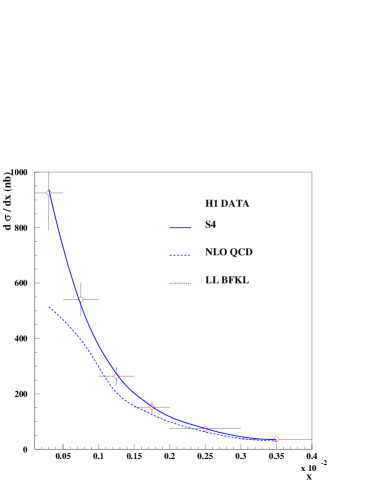
Figure 1: Comparison between the H1 $d\sigma/dx$ measurement with predictions for BFKL-LL, BFKL-NLL and DGLAP NLO calculations (see text). S4 and LL BFKL cannot be distinguished on that figure.

Following the successful BFKL [2] parametrisation of the forward-jet cross-section $d\sigma/dx$ at Leading Order (LO) at HERA [3, 4], it is possible to perform a similar study using Next-to-leading (NLL) resummed BFKL kernels. This method can be used for forward jet production at HERA in particular, provided one takes into account the proper symmetric two-scale feature of the forward-jet problem, whose scales are in this case $Q^{2},$ for the lepton vertex and $k_{T}^{2},$ for the jet vertex. In this short report, we will only discuss the phenomelogical aspects and all detailed calculations can be found in Ref. [5] for forward jets at HERA and in Ref. [6] for Mueller Navelet jets at the Tevatron and the LHC.

1.1 BFKL NLL formalism

We perform a saddle point approximation of the BFKL NLL formalism and compare it with the H1 forward jet cross section measurements . The BFKL NLL [7] formalism reads:

$$\frac{d\sigma}{dx} = N\left(\frac{Q^{2}}{k_{T}^{2}}\right)^{\gamma}\alpha_{S}(k_{T}^{2})\alpha_{S}(Q^{2})~{}\sqrt{A}~{}\exp\left(\alpha_{S}(k_{T}Q)\frac{N_{C}}{\pi}\chi_{eff}(\gamma_{C})\log(\frac{x_{J}}{x})\right)$$

$$\exp\left(-A\alpha_{S}(k_{T}Q)\log^{2}(\sqrt{\frac{Q}{k_{T}}})\right)$$

with

$$A^{-1} = \frac{3\alpha_{S}(k_{T}Q)}{4\pi}\log\frac{x_{J}}{x}\chi_{eff}^{\prime\prime}(\gamma_{C})$$

$$\gamma = \gamma_{C}+\frac{\alpha_{S}(k_{T}Q)\chi_{eff}(\gamma_{C})}{2}$$

where the saddle point equation is $\chi_{eff}^{\prime}(\gamma_{c})=0$. The effective kernels $\chi_{eff}(p,\gamma,\bar{\alpha})$ are obtained from the NLL kernel by solving the implicit equation:

$$\chi_{eff}=\chi_{NLL}(p,\gamma,\bar{\alpha}\chi_{eff}).$$

The values of $\chi$ are taken at NLL [7] using different resummation schemes to remove spurious singularities defined as CCS, S3 and S4 [8]. Contrary to LL BFKL, it is worth noticing that the coupling constant $\alpha_{S}$ is taken using the renormalisation group equations, the only free parameter in the fit being the normalisation.

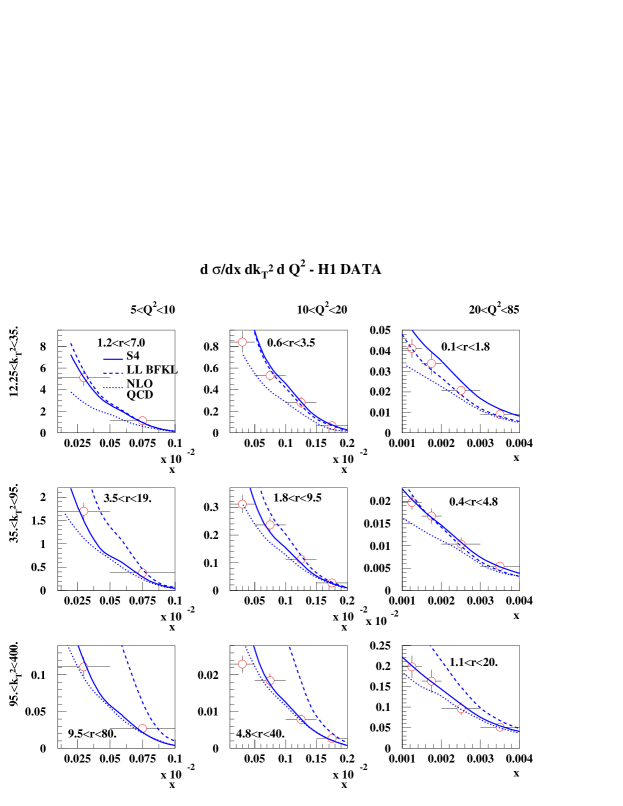
Figure 2: Comparison between the H1 measurement of the triple differential cross section with predictions for BFKL-LL, BFKL-NLL and DGLAP NLO calculations (see text).

One difficulty arises while fitting H1 $d\sigma/dx$ data [9] : we need to integrate the differential cross section on the bin size in $Q^{2}$, $x_{J}$ (the momentum fraction of the proton carried by the forward jet), $k_{T}$ (the jet transverse momentum), while taking into account the experimental cuts. To avoid numerical difficulties, we choose to perform the integration on the bin using the variables where the cross section does not change rapidly, namely $k_{T}^{2}/Q^{2}$, $\log 1/x_{J}$, and $1/Q^{2}$. Experimental cuts are treated directly at the integral level (the cut on $0.5<k_{T}^{2}/Q^{2}<5$ for instance) or using a toy Monte Carlo. More detail can be found about the fitting procedure in Appendix A of Ref. [4].

The NLL fits [5] can nicely describe the H1 data [9] for the S4 scheme ($\chi^{2}=5.6/5$ per degree of freedom with statistical errors only) whereas the S3 and CCS schemes show higher $\chi^{2}$. ($\chi^{2}=45.9/5$ and $\chi^{2}=20.4/5$ respectively with statistical errors only) The fit $\chi^{2}$ are good for all schemes if one considers statistical and systematics errors added in quadrature [3, 4]. The DGLAP NLO calculation fails to describe the H1 data at lowest $x$ (see Fig. 1).

The H1 collaboration also measured the forward jet triple differential cross section [9] and the results are given in Fig. 2. The BFKL LL formalism leads to a good description of the data when $r=k_{T}^{2}/Q^{2}$ is close to 1 and deviates from the data when $r$ is further away from 1. This effect is expected since DGLAP radiation effects are supposed to occur when the ratio between the jet $k_{T}$ and the virtual photon $Q^{2}$ are further away from 1. The BFKL NLL calculation including the $Q^{2}$ evolution via the renormalisation group equation leads to a good description of the H1 data on the full range. We note that the higher order corrections are small when $r\sim 1$, when the BFKL effects are supposed to dominate. By contrast, they are significant as expected when $r$ is different from one, ie when DGLAP evolution becomes relevant. We notice that the DGLAP NLO calculation fails to describe the data when $r\sim 1$, or in the region where BFKL resummation effects are expected to appear.

2 Mueller Navelet jets at the Tevatron and the LHC

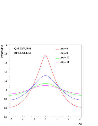
Figure 3: Azimuthal correlations between jets with $\Delta\eta=$6, 8, 10 and 11 and $p_{T}>5$ GeV in the CDF acceptance. This measurement will represent a clear test of the BFKL regime.

Mueller Navelet jets are ideal processes to study BFKL resummation effects [10]. Two jets with a large interval in rapidity and with similar tranverse momenta are considered. A typical observable to look for BFKL effects is the measurement of the azimuthal correlations between both jets. The DGLAP prediction is that this distribution should peak towards $\pi$ - ie jets are back-to-bacl- whereas multi-gluon emission via the BFKL mechanism leads to a smoother distribution. The relevant variables to look for azimuthal correlations are the following:

$$\Delta\eta = y_{1}-y_{2}$$

$$y = (y_{1}+y_{2})/2$$

$$Q = \sqrt{k_{1}k_{2}}$$

$$R = k_{2}/k_{1}$$

The azimuthal correlation for BFKL reads:

$$2\pi\left.\frac{d\sigma}{d\Delta\eta dRd\Delta\Phi}\right/\frac{d\sigma}{d\Delta\eta dR}=1+\frac{2}{\sigma_{0}(\Delta\eta,R)}\sum_{p=1}^{\infty}\sigma_{p}(\Delta\eta,R)\cos(p\Delta\Phi)$$

where in the NLL BFKL framework,

$$\sigma_{p} = \int_{E_{T}}^{\infty}\frac{dQ}{Q^{3}}\alpha_{s}(Q^{2}/R)\alpha_{s}(Q^{2}R)\left(\int_{y_{<}}^{y_{>}}dyx_{1}f_{eff}(x_{1},Q^{2}/R)x_{2}f_{eff}(x_{2},Q^{2}R)\right)$$

$$\int_{1/2-\infty}^{1/2+\infty}\frac{d\gamma}{2i\pi}R^{-2\gamma}\ e^{\bar{\alpha}(Q^{2})\chi_{eff}(p,\gamma,\bar{\alpha})\Delta\eta}$$

and $\chi_{eff}$ is the effective resummed kernel. Computing the different $\sigma_{p}$ at NLL for the resummation schemes S3 and S4 allowed us to compute the azimuthal correlations at NLL. As expected, the $\Delta\Phi$ dependence is less flat than for BFKL LL and is closer to the DGLAP behaviour [6]. To illustrate this result, we give in Fig. 3 the azimuthal correlation in the CDF acceptance. The CDF collaboration installed the mini-Plugs calorimeters aiming for rapidity gap selections in the very forward regions and these detectors can be used to tag very forward jets. A measurement of jet $p_{T}$ with these detectors would not be possible but their azimuthal segmentation allows a $\phi$ measurement. In Fig. 2, we display the jet azimuthal correlations for jets with a $p_{T}>5$ GeV and $\Delta\eta=$6, 8, 10 and 11. For $\Delta\eta=$11, we notice that the distribution is quite flat, which would be a clear test of the BFKL prediction. Similar measurements are possible at the LHC and predictions can be found in Ref. [6].

References

-
[1]
Slides:
http://indico.cern.ch/contributionDisplay.py?contribId=47&sessionId=8&confId=9499 - [2] L. N. Lipatov, Sov. J. Nucl. Phys. 23 (1976) 338; E. A. Kuraev, L. N. Lipatov and V. S. Fadin, Sov. Phys. JETP 45 (1977) 199; I. I. Balitsky and L. N. Lipatov, Sov. J. Nucl. Phys. 28 (1978) 822.
- [3] J.G. Contreras, R. Peschanski and C. Royon, Phys. Rev. D62 (2000) 034006; C. Marquet, R. Peschanski and C. Royon, Phys. Lett. B599 (2004) 236.
- [4] C. Marquet and C. Royon, Nucl. Phys. B739 (2006) 131.
- [5] O. Kepka, C. Marquet, R. Peschanski and C. Royon, preprints hep-ph/0609299, hep-ph/0612261; A. Sabio Vera and F. Schwennsen, hep-ph/0702158.
- [6] C. Marquet, C. Royon, preprint arXiv:0704.3409
- [7] V.S. Fadin and L.N. Lipatov, Phys. Lett. B429 (1998) 127; M. Ciafaloni, Phys. Lett. B429 (1998) 363; M. Ciafaloni and G. Camici, Phys. Lett. B430 (1998) 349.
- [8] G.P. Salam, JHEP 9807 (1998) 019; M. Ciafaloni, D. Colferai and G.P. Salam, Phys. Rev. D60 (1999) 114036; JHEP 9910 (1999) 017.
- [9] A. Aktas et al [H1 Collaboration], Eur. Phys. J. C46 (2006) 27.
- [10] A.H. Mueller and H. Navelet, Nucl. Phys. B282 (1987) 727.