A Constant Spectral Index for Sagittarius A* During Infrared/X-ray Intensity Variations

Abstract

We report the first time-series of broadband infrared color measurements of Sgr A*, the variable emission source associated with the supermassive black hole at the Galactic Center. Using the laser and natural guide star adaptive optics systems on the Keck II telescope, we imaged Sgr A* in multiple near-infrared broadband filters with a typical cycle time of $\sim$3 min during 4 observing runs (2005–2006), two of which were simultaneous with Chandra X-ray measurements. In spite of the large range of dereddened flux densities for Sgr A* (2 to 30 mJy), all of our near-infrared measurements are consistent with a constant spectral index of $\alpha$ = -0.6 $\pm$ 0.2 ($F_{\nu}\propto\nu^{\alpha}$). Furthermore, this value is consistent with the spectral indices observed at X-ray wavelengths during nearly all outbursts; which is consistent with the synchrotron self-Compton model for the production of the X-ray emission. During the coordinated observations, one infrared outburst occurs $\leq$36 min after a possibly associated X-ray outburst, while several similar infrared outbursts show no elevated X-ray emission. A variable X-ray to IR ratio and constant infrared spectral index challenge the notion that the infrared and X-ray emission are connected to the same electrons. We, therefore, posit that the population of electrons responsible for both the IR and X-ray emission are generated by an acceleration mechanism that leaves the bulk of the electron energy distribution responsible for the infrared emission unchanged, but has a variable high-energy cutoff. Occasionally a tail of electrons $\gtrsim$ 1 GeV is generated, and it is this high-energy tail that gives rise to the X-ray outbursts. One possible explanation for this type of variation is from the turbulence induced by a magnetorotational instability, in which the outer scale length of the turbulence varies and changes the high-energy cutoff.

1. Introduction

Since its discovery, the compact radio source, Sagittarius A* (catalog ), at the center of the Milky Way (Balick & Brown, 1974), now associated with a 3.7 $\times$ 10⁶ M_☉  supermassive black hole (Schödel et al., 2003; Ghez et al., 2003, 2005a), has been noted for its unusual emission properties. Detections of emission from Sgr A* at X-ray (Baganoff et al., 2003) and infrared (IR; Genzel et al. 2003b; Ghez et al. 2004, 2005b; Eckart et al. 2004) wavelengths have offered new probes into the central engine of our Galaxy. One of the challenges for models of this notably low luminosity source (10³⁶ erg s^-1 or, equivalently, 10^-9 L_Eddington) is to account for the relationship, if any, between emission at different wavelengths. Current models typically assume that all the emission originates either in an accretion flow onto the supermassive black hole or in an associated outflow (e.g., Falcke & Markoff, 2000; Melia et al., 2000; Yuan et al., 2002). The radio and IR photons are then presumed to be generated as synchrotron emission from a highly energetic population of electrons and the X-ray photons are produced by a combination of bremsstrahlung emission plus either a continuation of the radio/IR synchrotron emission or a synchrotron self-Compton component (SSC) of the radio/IR emission (e.g., Baganoff et al., 2001; Markoff, Falcke, Yuan, & Biermann, 2001; Liu & Melia, 2002; Quataert, 2002; Yuan et al., 2003).

A new constraint on the origin of Sgr A*’s emission has come from the observed variations in its emission properties as a function of time. At radio wavelengths, only modest emission variations of a factor of two at most, and only occasionally that much, have been detected on time scales from several hours to months (e.g., Falcke, 1999; Bower et al., 2002; Zhao et al., 2003; Herrnstein et al., 2004; Mauerhan et al., 2005). In contrast, dramatic variations have been seen in the intensity of the X-ray emission, with bursts that increase the X-ray emission by factors as large as $\sim$160, that last roughly an hour, and that occur about once a day (Baganoff et al., 2001, 2002; Goldwurm et al., 2003; Porquet et al., 2003). At near-infrared wavelengths, the emission varies on many different time scales ranging from minutes to hours (Genzel et al., 2003b; Eckart et al., 2004, 2006a; Clénet et al., 2004, 2005; Eisenhauer et al., 2005; Ghez et al., 2004, 2005b; Gillessen et al., 2006; Krabbe et al., 2006; Yusef-Zadeh et al., 2006). For infrared outbursts lasting approximately an hour (including both a rise and fall of the intensity), early 2 µm studies estimate a flare frequency of 4 $\pm$ 2 times per day for outbursts with peak intensities between 5–15 mJy (Genzel et al., 2003b; Eckart et al., 2006a) and more recent work at longer wavelengths (3.8 µm) indicate that peaks may occur up to 10 times per day (Hornstein, 2007). Coordinated infrared and X-ray observing campaigns have led to the detection of five additional X-ray outbursts, all of which are roughly coincident in time with infrared peaks (Eckart et al., 2004, 2006a; Yusef-Zadeh et al., 2006). However, these outbursts show a wide range of X-ray to IR peak ratios. This could be attributed to changes in the infrared spectral index (e.g., Yuan et al., 2004; Liu et al., 2006a; Yusef-Zadeh et al., 2006; Bittner et al., 2006). Recent measurements have suggested variations of the near-infrared spectral index, $-4\lesssim\alpha\lesssim 1$, where $F_{\nu}\propto\nu^{\alpha}$, with Sgr A* possibly becoming bluer when it is brighter (Ghez et al., 2005b; Eisenhauer et al., 2005; Gillessen et al., 2006; Krabbe et al., 2006). However, all but one of the IR spectral index measurements have so far been made with spectroscopy, which is a challenging measurement given the short wavelength bandpasses, low emission levels, rapid time variations, and high local stellar densities. Furthermore, none of the infrared spectral index measurements have been made, so far, in coordination with observations at other wavelengths.

An important first step in determining the physical cause of these outbursts is to reliably identify the emission processes responsible for creating the photons observed at various wavelengths. By measuring multiple properties of the outbursts (e.g., intensity levels and spectral indices) at multiple wavelengths (both during high and low emission states), a clearer picture will emerge. For example, if the X-ray emission is due to the same synchrotron process invoked for the IR emission, then the spectral index from IR to X-ray wavelengths should be the same (and thus the IR/X-ray peak ratio would reveal the same spectral index). On the other hand, an SSC model for the X-ray emission would require that the typical spectral indices of the synchrotron (IR) and SSC (X-ray) emission match each other, while the IR-to-X-ray spectral index could vary.

In this paper, we present the first time-series measurements of Sgr A*’s broadband infrared ($H-K^{\prime}$ and $K^{\prime}-L^{\prime}$) colors, which were obtained with the laser guide star adaptive optics system (LGS AO) on the W. M. Keck II 10-meter telescope and most of which were taken simultaneously with X-ray observations from the Chandra X-Ray Observatory. By comparing to spectroscopically identified stars in the Galactic Center, these broadband colors can be converted into spectral indices for Sgr A*. Additional natural guide star adaptive optics (NGS AO) Keck observations of Sgr A*’s $L^{\prime}-M_{s}$ colors are also reported. The observations, data analysis, and results are described in §2 and §3, for the IR and X-ray measurements, respectively. These measurements show that, while large changes in the intensity of the infrared emission are detected, the infrared spectral index is constant throughout all of our observations. In §4 we discuss the implications these findings have on current models. In particular, we argue that these observations support the SSC model for the production of the 2–8 keV emission and that a variable high-energy cutoff of the acceleration process would be required to generate a variable IR/X-ray intensity ratio while maintaining constant and equal IR and X-ray outburst spectral indices.

2. Keck Near-Infrared Adaptive Optics Data

2.1. Near-Infrared Observations

On 2005 July 31 and 2006 May 2 (UT), Galactic Center observations in the $H$ ($\lambda_{o}$ = 1.63 µm, $\Delta\lambda$=0.30 µm), $K^{\prime}$ ($\lambda_{o}$ = 2.12 µm, $\Delta\lambda$ = 0.35 µm), and $L^{\prime}$ ($\lambda_{o}$ = 3.78 µm, $\Delta\lambda$=0.70 µm) photometric bandpasses were conducted using the facility near-infrared camera, NIRC2 (K. Matthews et al. 2006, in preparation) behind the laser guide star AO system (Wizinowich et al., 2006; van Dam et al., 2006) on the W. M. Keck II 10-meter telescope. With the narrow-field camera of NIRC2 (9.93 mas pixel^-1), the 1024 $\times$ 1024 pixel InSb array provides a field of view of 10$\farcs$2 $\times$ 10$\farcs$2. USNO-A2.0 0600-28577051 (catalog ) (R = 13.7 mag and $\Delta$$r_{Sgr~{}A*}=19\arcsec$) was used during the observations to provide information on the tip/tilt term of atmospheric aberrations, which can not be derived from the laser guide star. For more details regarding the general LGS AO performance on the Galactic Center, see Ghez et al. (2005b). Measurements made on the night of 2005 July 31 with only the tip/tilt loops closed on a bright star at zenith yielded a seeing measurement of $\sim$0$\farcs$18 at 2 µm (which corresponds, theoretically, to 0$\farcs$23 at the Galactic Center airmass of 1.52). Seeing conditions on the night of 2006 May 2 were much less favorable and conditions were extremely variable throughout the night (in fact, due to the much poorer atmospheric conditions, setup for the LGS AO system was sufficiently time consuming that no official seeing measurement was made). As such, only observations made at airmass $\lesssim$1.54 are usable for the 2006 May 2 observations. Resolutions (full widths at half maximum) and Strehls for both epochs can be found in Table 1. In order to optimize observing efficiency and eliminate any induced variability due to dithering, Sgr A* was placed in an area of the detector free from bad pixels and held fixed throughout the observations. Observations were made by cycling through the $H$ (t_exp = 7.4 s $\times$ 3 coadds), $K^{\prime}$ (t_exp = 2.8 s $\times$ 10 coadds), and $L^{\prime}$ (t_exp = 0.5 s $\times$ 60 coadds) filters repeatedly for 113 minutes in 2005 and 52 minutes in 2006, with a three-filter cycle completed approximately every three minutes. On 2005 July 31, these observations were interrupted briefly (9 min) due to the requirement that the laser be shuttered when its beam crosses the field of view of another telescope on Mauna Kea. Observations of a relatively dark portion of the sky were conducted after the Galactic Center observations to measure the background emission. In order to reduce the effects of thermal emission from dust on the warm image rotator mirror inside the AO enclosure, background images at $L^{\prime}$ were obtained at two-degree increments covering the full range of physical angles of the rotator mirror during the Galactic Center observations.

Additional $K^{\prime}$ and $L^{\prime}$ NIRC2/LGS AO observations of the Galactic Center were made on 2006 July 17 (UT). Integration times and coadds were the same as the 2005 July 31 epoch but during these observations, the telescope was dithered semi-randomly within a box 0$\farcs$7 on a side centered on Sgr A* with 3 pairs of $K^{\prime}$ and $L^{\prime}$ images taken at each dither position. Resolutions and Strehls were comparable to the 2005 July 31 night and measurements on a bright star at zenith yielded a seeing of 0$\farcs$35 at 2 µm (see Table 1). These observations lasted approximately 187 minutes with a 16 minute outage in the middle due to a technical problem with the LGS AO system. Observations of the background sky/thermal emission were accomplished in an identical manner to the observations described above.

Complementary adaptive optics images of the Galactic Center were obtained on 2005 July 16 (UT) using NIRC2 and the AO system in its natural guide star mode (Wizinowich et al., 2000). USNO-A2.0 0600-28577051 was again used but this time to provide information on all terms of the atmospheric aberrations. Observations in the $L^{\prime}$ and $M_{s}$ ($\lambda_{o}$ = 4.67 µm, $\Delta\lambda$ = 0.24 µm) photometric bandpasses were interleaved by cycling through a 3 position, 0$\farcs$5 dither pattern on the array (to avoid dithering Sgr A* into the noisy, bottom-left quadrant of the array), in which two $L^{\prime}$ (t_exp = 0.5 s $\times$ 120 coadds) and three $M_{s}$ (t_exp = 0.2 s $\times$ 600 coadds) exposures were taken at each position. While 0.2 s exposures are technically possible using the full size of the array, sub-arraying to 512 $\times$ 512 pixels greatly improves the observing efficiency at $M_{s}$ and was used for all exposures on this night. Again, observations of the background sky/thermal emission were taken at multiple rotator mirror angles after the GC observations. Additionally, $M_{s}$ photometric standard stars HD 1881 ($M_{s}$ = 7.17 $\pm$ 0.02), HD 3029 (7.70 $\pm$ 0.02), and SAO 3440 (7.04 $\pm$ 0.02) were observed in order to calibrate the $M_{s}$ images (Leggett et al., 2003). Table 1 summarizes all of the Galactic Center IR observations presented here.

2.2. Near-Infrared Data Analysis

The standard image reduction steps of background subtraction, flat-fielding, bad pixel repair, and optical distortion correction were carried out on each exposure. As in Ghez et al. (2005b), the best background subtraction at longer wavelengths ($L^{\prime}$ and $M_{s}$), for both the LGS and NGS data, was achieved by subtracting, from each exposure, the average of three sky exposures that were taken at similar rotator angles. Since the narrow-field camera of NIRC2 oversamples the point-spread function (PSF) at all wavelengths (see Table 1), all images were binned by a factor of two for computational efficiency. Additionally, due to the lower signal-to-noise ratio (SNR) of the NGS AO data, each $M_{s}$ image was made by averaging six individual exposures while each $L^{\prime}$ image was made of four individual exposures (two taken between, and one on either side of, the corresponding two sets of $M_{s}$ exposures.)

Identification and characterization of point sources is accomplished using StarFinder, an IDL PSF-fitting package developed for astrometry and photometry in crowded stellar fields (Diolaiti et al., 2000). StarFinder is first run on an average image made from all the data taken on each night as well as on images made from three independent, equal-quality subsets of the data for each bandpass. Sources having a range of intensities are selected in StarFinder in order to determine the PSF in the images. The brightest stars, whose cores are in the non-linear regime of the detector ($>$12,000 counts), are used to generate the PSF wings while fainter sources are used to produce the PSF core. For each bandpass, any source that is detected in the average image (with a correlation value of $\geq$0.8 in the 2005 July and 2006 July data and $\geq$0.6 in the 2006 May and 2005 July data) as well as at least two out of the three subsets (correlation $\geq$0.6 and $\geq$0.4 for the two groupings mentioned previously) is considered a ‘validated’ source. This list of sources is then used as the input detection list for a modified version of StarFinder, run on the individual images, that allows the intensity of the sources to vary but holds their positions fixed.

Images are photometrically calibrated using the apparent magnitudes of several of the brightest stars in each image. Specifically, we use measurements of IRS 16C ($H$ = 11.99, K = 9.83, $L^{\prime}$ = 8.14 mag) and IRS 16NW ($H$ = 12.04, K = 10.03, $L^{\prime}$ = 8.43 mag), from Blum et al. (1996) at $H$ and $K^{\prime}$ and S. A. Wright et al. (2007, in preparation) at $L^{\prime}$, which have estimated uncertainties of $\sim$4%, 4%, and 5% at $H$, $K^{\prime}$, and $L^{\prime}$, respectively. Using the observed $M_{s}$ photometric standards, we calibrate IRS 16C ($M_{s}$ = 8.08) and IRS 16NW ($M_{s}$ = 8.41) in the average $M_{s}$ image for the night and then use them as secondary calibrators for the individual images. Absolute calibration uncertainties at $M_{s}$ are estimated to be $\sim$9%. Determination of the uncertainties in the relative photometry of Sgr A*, at all wavelengths, is carried out as in Ghez et al. (2005b) by calculating the RMS flux density variations between images for non-variable stars of comparable magnitude. Dereddened flux densities are calculated assuming a visual extinction of 29 $\pm$ 1 mag from S. A. Wright et al. (2007, in preparation) and an extinction law derived by Moneti et al. (2001), and then converted to flux densities with zero points from Tokunaga & Vacca (2005, see footnotes in Table 1).

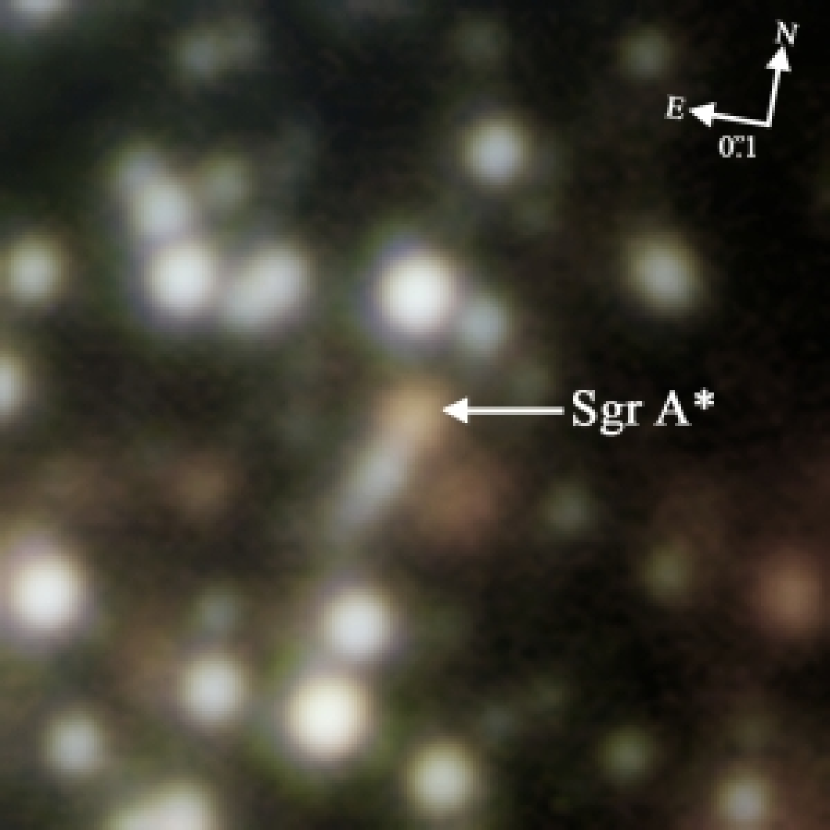
Figure 1.— Central 1″ $\times$ 1″ region of the Galactic Center. This false-color image is constructed from the average $H$ (blue), $K^{\prime}$ (green) and $L^{\prime}$ (red) images taken on 2005 July 31 with the LGS AO system. The high density of stars seen in this image shows the need for a robust detection algorithm in order to remove their contaminating emission, which is much bluer than Sgr A*’s, and thereby to obtain an accurate measurement of Sgr A*. The red emission immediately to the SW of Sgr A* has been previously identified as a dust feature projected along the line of sight toward Sgr A* (Ghez et al., 2005b).

The IR spectral indices are calculated from Sgr A*’s observed colors and the relative interstellar reddening (color excess) inferred from nearby stars. With this approach, the equation for the spectral index, $\alpha$ (defined as $F_{\nu}\propto\nu^{\alpha}$), is

$$\alpha_{\lambda_{1}-\lambda_{2}}=\frac{-0.4[(m_{\lambda_{1}}-m_{\lambda_{2}})_{obs}-E(\lambda_{1}-\lambda_{2})]+log(\frac{f_{0,\lambda_{1}}}{f_{0,\lambda_{2}}})}{log(\frac{\lambda_{2}}{\lambda_{1}})},$$ (1)

where $m_{\lambda_{n}}$ is the apparent magnitude of Sgr A* at $\lambda_{n}$, E($\lambda_{1}-\lambda_{2}$) is the color excess measured from nearby stars, and $f_{0,\lambda_{n}}$ is the flux density of a 0 mag star at $\lambda_{n}$. Sgr A*’s colors are derived from flux density estimates that have the same time center. For the LGS AO data, this is achieved by interpolating the flux densities at $K^{\prime}$-band as a function of time to the flux density at the time of the nearest measurement within the $H$- or $L^{\prime}$-band. In all cases the difference between the time of the measurement and the time to which the measurement is interpolated is always less than 81 s. Since each pair of average $L^{\prime}$ and $M_{s}$ images in the NGS AO data set are centered on the same time, no interpolation is necessary. By dereddening the apparent colors of Sgr A* with the color excesses of nearby stars (see Appendix), we avoid systematics associated with uncertainties in the extinction law or photometric zero points.

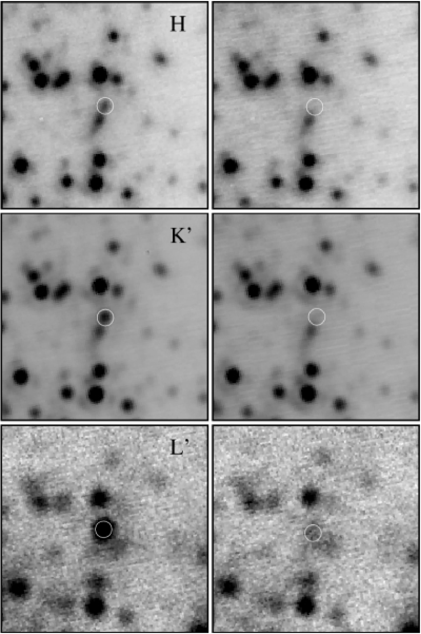
Figure 2.— 1″ $\times$ 1″ images showing Sgr A* (white circle) at its highest (left) and lowest (right) states in $H$, $K^{\prime}$, and $L^{\prime}$ on 2005 July 31 taken at 07:57 and 08:32 (UT), respectively. The maximum and minimum recorded values are 9, 12, 15 mJy and 3, 2, 3 mJy at $H$, $K^{\prime}$, and $L^{\prime}$, respectively. The StarFinder PSF-fitting routine consistently detects a point source at the location of Sgr A* at all three wavelengths with correlation values of $>$0.7.

2.3. Near-Infrared Results

Figure 1 shows a color composite of the central 1″ $\times$ 1″ $H$, $K^{\prime}$, & $L^{\prime}$ images from 2005 July 31. This image shows the high density of stars surrounding Sgr A*, necessitating that the flux from all stars of comparable brightness to Sgr A* be accounted for. This is especially important when the emission from Sgr A* is at its lowest levels, as shown in the right panel of Figure 2.

During our observations, Sgr A* exhibits a wide range of flux densities as shown in Figure 3, which displays the dereddened light curves of Sgr A* and comparison stars for all of the 2005 and 2006 observations. During our 2005 LGS AO observations on July 31, Sgr A*’s light curve shows two clear minima, with values of 2-3 mJy in all three filters, separating emission events that can be associated with three distinct peaks. However, only one maximum is observed in its entirety with peak levels of 9, 12, and 15 mJy in the $H$, $K^{\prime}$, and $L^{\prime}$ filters, respectively. During our 2005 July 16 observations, Sgr A* starts out in a low state of 3 and 2 mJy at $L^{\prime}$ and $M_{s}$, respectively, and rises to 7 mJy in both filters by the middle of the observations. While the 2006 May data set has the poorest image quality, it is a particularly interesting observation because Sgr A* is then detected in its highest IR outburst intensity measured to date. At the beginning of the observations, Sgr A* is measured at dereddened fluxes of 23, 27, and 30 mJy in the $H$, $K^{\prime}$, and $L^{\prime}$ filters, respectively. In the following 52 minutes, it falls to approximately 13 mJy in all three filters. In the 2006 July LGS AO observations, Sgr A*’s light curve shows a decaying flank from the outset, starting out at 7 and 8 mJy in the $K^{\prime}$ and $L^{\prime}$ filters and falling to 2-3 mJy in both filters over the course of 50 minutes. At the very end of these observations, the beginning of yet another outburst event can be seen.

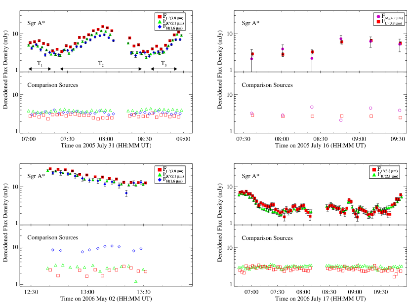
Figure 3.— Light curves for Sgr A* and nearby comparison stars of similar brightness at each wavelength for 2005 July 31 (LGS AO; top left), 2005 July 16 (NGS AO; top right), 2006 May 2 (LGS AO; bottom left), and 2006 July 17 (LGS AO; bottom right). In all but 2006 May 2, the comparison sources are chosen to match the measurements of Sgr A* at its minimum values: S0-37 (ID8 in Schödel et al. 2003) at $H$ and $K^{\prime}$, S0-17 at $L^{\prime}$, and S0-1 at $M_{s}$. (In the lower quality 2006 May 2 images, S0-37 was not detected in the $H$-band images and has been replaced with S0-17.) Over four epochs, many outbursts are detected, including three separate events during the 2005 July 31 observations, marked as T₁, T₂, and T₃.

Sgr A*’s spectral index appears to be independent of flux density. This is most clearly seen in the spectral indices derived from the dereddened $K^{\prime}-L^{\prime}$ colors, since measurements from $H-K^{\prime}$ suffer from stellar background contamination (see discussion below) and those from $L^{\prime}-M_{s}$ have a much lower SNR due to the high thermal background at $M_{s}$. Figure 4 shows the stability of $\alpha_{K^{\prime}-L^{\prime}}$ over flux density variations spanning multiple outburst events. The plotted uncertainties only incorporate those of the relative flux density measurements of Sgr A*. Within the three runs in which $K^{\prime}-L^{\prime}$ was measured, the spectral index is constant with flux density. The larger spread of $\alpha$ at flux densities below 4 mJy in 2006 July compared to 2005 July is most likely a consequence of the poorer image quality, which increases the effects of background contamination at low flux levels. For the run with the highest image quality, the spectral index is consistent with a constant value to within 29% over intensities ranging from 2 – 12 mJy. Even with the poorer seeing conditions in the 2006 May observations, which span the largest change in flux densities (11 – 27 mJy), the spectral index is constant to within 19%.

Figure 4.— Spectral index ($F_{\nu}\propto\nu^{\alpha}$) vs. Sgr A* flux density derived from $K^{\prime}-L^{\prime}$ on 2005 July 31 (top), 2006 May 2 (middle), and 2006 July 17 (bottom). Within the measured uncertainties, Sgr A*’s spectral index shows no variation with intensity over multiple outburst events. The absolute uncertainty show in each plot is derived from the uncertainty in the color excess correction (see Appendix).

Sgr A*’s spectral index is also constant over wavelengths ranging from 1.6 – 4.7 microns. At shorter wavelengths, the spectral indices derived at flux densities below 4 mJy show a trend blueward with decreasing intensity (See Figure 5, left). Since this effect is not seen at the longer wavelengths, we attribute this effect to contamination from the underlying stellar population (which is much bluer than Sgr A*; see Figure 1). To investigate this in more detail, this local background contamination is removed from the $H-K^{\prime}$ measurements by subtracting off the minimum level observed at the position of Sgr A* during the observations, which is taken to be the average level detected during a 10 minute period in the first observed minimum beginning at $\sim$07:20 for the 2005 July data set and the average of the last three points for the 2006 May data set. With this approach, the 2005 $H-K^{\prime}$ spectral indices are not only constant with respect to outburst intensity (see Figure 5, right), but also consistent with the results from longer wavelengths shown in Figure 4 and Table 2. Applying this subtraction technique to the longer wavelength measurements in 2005 July ($K^{\prime}-L^{\prime}$ and $L^{\prime}-M_{s}$) results in no significant change in the spectral indices; thus supporting the hypothesis that the contaminating background is from the blue stellar population. A similar trend is seen in the 2006 May $H-K^{\prime}$ and $K^{\prime}-L^{\prime}$ measurements. We, therefore, correct only the $H-K^{\prime}$ spectral indices for local background contamination.

Figure 5.— (Left) Spectral index, $\alpha$ ($F_{\nu}\propto\nu^{\alpha}$) vs. Sgr A* flux density derived from $H-K^{\prime}$ on 2005 July 31 before the background contamination has been removed. While the higher flux densities show the same stability trend as $\alpha_{K^{\prime}-L^{\prime}}$, the spectral indices derived below 4 mJy are much bluer, which we attribute to contamination from the underlying stellar population. (Right) The same spectral indices after the background contamination is removed by subtracting the average level of emission during the first minimum ($H$=3.2 $\pm$ 0.2, $K^{\prime}$=2.8 $\pm$ 0.1, $L^{\prime}$=3.6 $\pm$ 0.2 mJy). While the errors have increased due to the subtraction technique, these spectral indices are consistent with the spectral indices at other wavelengths.

Table 2 presents the weighted average of $\alpha$ derived from various wavelength pairs over multiple observing runs, including a recalculation of the spectral index for one pair of $K^{\prime}$/$L^{\prime}$ observations in 2004 (Ghez et al. 2005b). The reported uncertainties include the propagated uncertainties of the observed color of Sgr A* as well as the uncertainties from the dereddening method. All of these measurements are consistent with each other within their uncertainties and, when averaged together, imply a spectral index for Sgr A* during these observations of -0.63 $\pm$ 0.16 (where we have taken the weighted average of the three different color pairs from Table 2 after quadratically summing the two sources of error). This spectral index appears to be independent of intensity (F_IR = 2 – 30mJy), time (multiple outbursts over three years), or wavelength (1.6 – 4.7 microns).

Several comments can be made about these results when compared to previous results in the literature. While photometrically derived spectral indices of Sgr A* are obtained in an inherently different manner than those obtained directly from spectra, they agree within approximately two sigma with OSIRIS K-band (2.02–2.38 µm) spectra obtained at a comparable emission level (i.e., $\alpha$ = -2.6 $\pm$ 0.9 when F${}_{Sgr~{}A*}$ = 6.1 mJy; Krabbe et al. 2006). Other results from SINFONI K-band spectra (1.95–2.45 µm) which suggest a correlation of spectral index with emission intensity (Gillessen et al., 2006) are not as discrepant as they may seem. Of the three methods presented by the Gillessen et al., the ‘off state subtraction’ method, which most closely resembles the method presented here, results in a data set that is statistically consistent with no spectral index/intensity correlation down to 2 mJy, and that method gives $\alpha_{bright~{}state}=-0.6\pm 0.2$, which is in excellent agreement with the value that we derive above. The apparent correlation seen from the other two methods may be explained by the local background contamination that becomes significant at flux densities below 4 mJy. A local aperture background at K-band could sample the contamination from the surrounding population of blue stars and the subtraction of an overly blue background would lead to a redder appearance for Sgr A* at low levels, where the background emission becomes comparable to Sgr A*’s intrinsic emission. Furthermore, $\alpha_{preflare}$ from Gillessen et al., as well as the spectral indices presented by Eisenhauer et al. (2005), reporting extremely red spectral indices for Sgr A* ($\alpha\lesssim-3$), were made at very low flux levels (F $\lesssim$ 2 mJy), where the complications with the background make this a very challenging measurement to make. Therefore, we suggest that the apparent variation in the IR color of Sgr A* found in previous experiments could arise as a consequence of background contamination in this extremely crowded field.

3. Chandra X-ray Data

3.1. ACIS X-ray Observations and Data Analysis

X-ray observations of the Galactic Center were conducted with the Chandra X-Ray Observatory (Weisskopf et al., 1996) using the imaging array of the Advanced CCD Imaging Spectrometer (ACIS-I; Garmire et al. 2003) from 2005 July 30 19:44 – 2005 July 31 09:10 and 2006 July 17 04:17 – 2006 July 17 12:37 (UT). The last two hours of the 2005 observations and three hours of the 2006 observations overlapped with the Keck LGS AO observations from the ground. The data were acquired and reduced as described by Baganoff et al. (2001, 2003) (see also Eckart et al., 2004, 2006a). Briefly, the instrument was operated in timed exposure mode with detectors I0-3 and S2 turned on. The time between CCD frames was 3.141 s and the event data were telemetered in faint format. The data were analyzed using the Chandra Interactive Analysis of Observations (CIAO) v3.2 software package with CALDB v3.1.0. Source counts in the 2–8 keV band were obtained from aperture photometry on Sgr A* using an aperture radius of 1$\farcs$5 and a surrounding sky annulus extending from 2″ to 4″, excluding regions around discrete sources and bright structures.

3.2. X-ray Results

Figure 6 shows the 2005 X-ray light curve marked with the period of overlapping Keck IR data. Figure 7 (top) shows the 2005 Keck light curves in the $H$-, $K^{\prime}$-, and $L^{\prime}$-bands along with the simultaneous part of the X-ray light curve. While a factor-of-twenty X-ray outburst is detected, it is not simultaneous with the Keck IR observations. Here we restrict our analysis to the period overlapping the Keck observations. A Bayesian blocks analysis, as described in Eckart et al. (2004), is performed on the X-ray light curve without background subtraction. This analysis indicates that Sgr A*’s X-ray light curve is consistent with no variability at the 90% confidence level during the entire remaining period after the main outburst. The mean count rate of the background-subtracted light curve from $\sim$23:00 - 07:00 is 4.29 $\pm$ 0.68 cts ks^-1 corresponding to a 2–8 keV luminosity of 1.8 $\pm$ 0.3 $\times$ 10³³ erg s^-1. During the Keck overlap, the mean count rate is 4.94 $\pm$ 1.54 cts ks^-1, which lies within the 90% confidence interval, computed according to Gehrels (1986), for the period cited above. Therefore, we adopt this 90% confidence interval as an upper limit during the Keck observations, corresponding to 2.1 $\times$ 10³³ erg s^-1. Thus, the X-ray luminosity does not change by more than $\sim$16% during the 2005 IR outburst observed with Keck.

Figure 6.— Chandra 2-8 keV light curve of 2005 July 30/31 including the overlap with ground-based Keck observations. The Chandra observations begin on 2005 July 30 20:15:12.0 and end on 2005 July 31 08:49:04.0 (UT). While one significant outburst is detected, peaking at $\sim$22:30 on July 30, it is not simultaneous with the Keck IR observations.

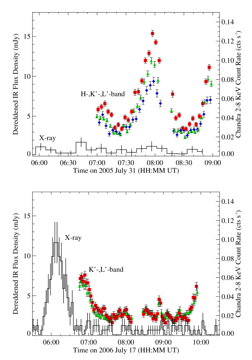
Figure 7.— The overlapping 2005 (top) and 2006 (bottom) IR (left axis) and X-ray (right axis) light curves (see Figure 3 for a description of the IR symbols). No significant X-ray variations occurred within $\sim$8.5 hours of the start of the 2005 IR observations. On the other hand, $\sim$36 minutes before the beginning of the 2006 IR observations, Chandra detected a factor of 20 outburst. As previous coordinated campaigns have detected IR variations persisting more than 36 minutes after the associated X-ray emission dropped below the constant level of the diffuse emission from within the central parsec (Eckart et al., 2004, 2006a), we associate the IR decay at the beginning of our IR observations with the X-ray outburst.

In 2006, a strong ($\sim$20$\times$) X-ray outburst is detected and it peaks at 4.0 $\times$ 10³⁴ erg s^-1 about 36 minutes before the Keck observations begin (Figure 7, bottom). While there is a non-negligible chance that the Keck IR outburst is unrelated to this X-ray event (10% given IR outbursts occurring four times a day, 25% for outbursts ten times per day) previous coordinated activity at IR and X-ray wavelengths have shown that the IR decay can persist 36 minutes (and longer) after the presumably associated X-ray peak (Eckart et al. 2004, Figure 4; Eckart et al. 2006a, Figure 9). Furthermore, all X-ray outbursts which have had simultaneous IR observations, have shown apparent associated IR outbursts. The probability of a second IR event occuring within 36 minutes of the X-ray peak (assuming that a unseen IR peak occurred simultaneously with the X-ray peak and our IR observations captured a second, unrelated outburst) is only 1%(6%) for outbursts occuring four (ten) times per day. This strengthens the possible association here. We note that the decreasing X-ray emission cannot be tracked for as long as the IR emission because of Chandra’s lower angular resolution combined with the bright, steady diffuse X-ray emission in the central parsec. Additionally, the flatness at the beginning of the IR light curve resembles short time-scale non-monotonic fluctuations that are seen in the structure of these other coordinated outbursts, and does not necessarily imply that a peak has occurred at the beginning of the IR observations. Thus, our data are consistent with no temporal displacement between the X-ray and IR peaks. It is, therefore, possible that the elevated IR state observed in our 2006 July observations is associated with the X-ray activity that immediately precedes it.

4. Discussion

Our observations show that Sgr A*’s infrared spectral index is constant, with a value of $\alpha$ = -0.6 $\pm$ 0.2 ($F_{\nu}\propto\nu^{\alpha}$). The lack of dependence upon intensity is quite notable, given the wide range of infrared intensities measured during our experiment (2–30 mJy). While our low points are comparable to some of the lowest measurements ever made of Sgr A*, the peak emission detected in this study is the highest infrared measurement recorded thus far (Genzel et al., 2003b; Eckart et al., 2004, 2006a; Clénet et al., 2004, 2005; Eisenhauer et al., 2005; Ghez et al., 2004, 2005b; Gillessen et al., 2006; Krabbe et al., 2006; Yusef-Zadeh et al., 2006). The IR emission is most likely from synchrotron photons, as demonstrated by the recent reports of polarized IR emission from Sgr A* (Eckart et al., 2006b; Meyer et al., 2006a, b). Our measured value of the spectral index of -0.6 indicates that the synchrotron emission is optically thin and arises from an electron energy distribution with $N(\gamma_{e})\propto\gamma_{e}^{-p}$, where $p$ = 1-2$\alpha$ = 2.2 and $\gamma_{e}$ is the Lorentz factor of the electrons. In order to associate particular electron energies, or $\gamma_{e}$, with the observed IR synchrotron emission, knowledge of the magnetic field strength is required ($\nu_{sync}=\frac{3}{4\pi}\gamma_{e}^{2}\frac{eB}{m_{e}c}$ and where E${}_{e}=\gamma_{e}m_{e}c^{2}$.) Although highly uncertain, if we adopt a magnetic field strength of B$\sim$20 G, as has been suggested by others (e.g., Markoff, Falcke, Yuan, & Biermann, 2001; Yuan et al., 2003), then $\sim$ GeV electrons ($\gamma_{e}\approx$2000) are responsible for producing the observed IR emission. It has been generally assumed that the intensity variations are caused by acceleration events, possibly caused by an enhancement of the mass accretion rate or magnetic reconnection events within the accreting gas, which enable electrons to reach such high energies (e.g., Markoff, Falcke, Yuan, & Biermann, 2001; Liu & Melia, 2002; Yuan et al., 2003, 2004; Liu et al., 2006a; Tagger & Melia, 2006). In order to produce IR intensity changes without changing the IR spectral index, the electron acceleration mechanism has to change only the total number of electrons in this energy range while leaving their overall energy distribution unchanged.

If the X-ray emission arises from inverse Compton scattering of synchrotron photons, then the X-ray spectral index should match that of the synchrotron emission. Examining the X-ray spectral indices from all previously reported outbursts, we find that the X-ray spectral indices are consistent (within two sigma) with the infrared spectral index derived here, in all but the most extreme X-ray outburst, and have $\langle\alpha_{X-ray}\rangle=-0.3\pm 0.6$. As the largest X-ray outburst dwarfs all other known X-ray outbursts by more than a factor of three (Porquet et al., 2003), this event may represent a very different scenario than is producing the more common X-ray events. Nevertheless, the similarity of the typical X-ray and IR spectral indices is completely consistent with the SSC model for the production of the X-ray photons.

In contrast to the uniformity of the infrared and X-ray spectral indices, the ratio of infrared to X-ray intensity appears to be quite variable. During our 2006 coordinated observations, decaying IR emission is seen in association with a significant X-ray outburst. In fact, all previous IR observations obtained during significant X-ray intensity variations have shown similar associations (Eckart et al., 2004, 2006a; Yusef-Zadeh et al., 2006). On the other hand, no elevated X-ray emission is seen during our 2005 coordinated observations, in spite of the large IR outburst that occurred then. Similar occurrences of IR peaks with no X-ray outbursts are reported by Yusef-Zadeh et al. (2006). Previously, the IR and X-ray photons have been theoretically linked through either a synchrotron or SSC mechanism and it has been shown that a variation in the ratio of X-ray to IR peak intensities would be accompanied by a change in the infrared spectral index or, equivalently, in the slope of the electron energy distribution (e.g., Yuan et al., 2004; Liu et al., 2006b; Bittner et al., 2006). Yusef-Zadeh et al. (2006) suggest that a variation in the magnetic field strength could be responsible for the variable IR/X-ray intensity ratio observed in the double peak structure seen during their coordinated observations (see Yusef-Zadeh et al. 2006, Figure 9). If the magnetic field is reduced in an event, for example, then there are two possible ways to account for the observed constancy of the spectral index. If the IR synchrotron photons Compton scatter off the $\sim$25 MeV electrons responsible for the submillimeter emission then a reduction in the magnetic field in the IR emitting region would result in a reduction of the infrared synchrotron emission and a proportional reduction of the X-ray SSC emission (and, thus, would display a constant IR/X-ray intensity ratio). If, on the other hand, the submillimeter photons are Compton scattered by the same $\sim$1 GeV electrons in the hot spot that produce the IR synchrotron emission, then a reduction in the magnetic field would result in the IR synchrotron only without changing the X-ray SSC emission and the IR/X-ray ratio would decrease. However, both of these are inconsistent with the observations.

The variation in the ratio of IR and X-ray peak intensities, despite a constant spectral index at both IR and X-ray wavelengths, suggests that one may not be able to connect the infrared and X-ray emission to the same electrons. Instead, we posit that while the acceleration mechanism leaves the bulk of the electron energy distribution unchanged, the upper energy cutoff ($\gamma_{max}$) is not constant over every event (a variation of which was explored by Yuan et al. 2004). In this scenario, the X-ray photons are produced by electrons that have higher energies (e.g. E$\gtrsim$1 GeV for B$\sim$20 G) than those that give rise to the IR synchrotron photons. These electrons can give rise to the X-ray emission in two ways. In one scenario, the electrons produce synchrotron emission that is upscattered off of the population of $\lesssim$25 MeV electrons responsible for the submillimeter emission. (These same low-energy electrons would scatter the near-IR photons in the observable IR bands to energies below 2 keV, which is undetectable by Chandra due to interstellar absorption.) In an alternative scenario, $\gtrsim$1 GeV electrons act as the scattering population for the submillimeter synchrotron photon field generated by the $\lesssim$25 MeV electrons and produce a similar level of observed X-ray activity (Yusef-Zadeh et al., 2006). In either case, the variation in X-ray emission is caused by the fact that these $\gtrsim$1 GeV electrons may not always be produced in the acceleration event if $\gamma_{max}$ is not high enough. A variable $\gamma_{max}$ could be the result of a variation of the largest turbulence scale sizes accompanying different instances of a disk instability. Therefore, it is this occasional high-energy population of electrons that gives rise to the relatively infrequent X-ray outbursts. Furthermore, as energies below $\gamma_{max}$ are always created during the acceleration event, X-ray outbursts, when present, would always show correlated infrared activity (as is the case with all current NIR observations during X-ray outbursts; Eckart et al. 2004, 2006a; Yusef-Zadeh et al. 2006). While this simple model can explain a constant IR/X-ray intensity ratio when conditions are suitable for creating the X-ray photons, physical parameters such as the magnetic field, source size, and electron density in the emitting region could easily change from outburst to outburst, resulting in a change in the IR/X-ray intensity ratio during coordinated outbursts (for example, the IR/X-ray spectral index between the two peaks seen by Yusef-Zadeh et al. 2006 changes by only $\sim$0.14). Additionally, as suggested by Yuan et al. (2004), a variable $\gamma_{max}$ could explain the anomalous, soft X-ray spectral index detected by XMM-Newton (Porquet et al., 2003).

5. Summary

The broadband infrared imaging method presented here, when combined with PSF fitting photometry, allows for robust measurements of the color of Sgr A* during an outburst due to the short, high quality images that can be taken throughout the event. By comparing with several spectroscopically identified stars, we are able to present spectral indices that are not dominated by the uncertainties in the interstellar reddening law. We find the most reliable spectral index measurements are obtained from the $K^{\prime}-L^{\prime}$ colors, due to the challenges associated with accounting for the blue stellar background when Sgr A* is its lowest emission states in the $H-K^{\prime}$ color; this challenge may also explain the discrepant spectral indices in the literature.

From observations taken between 2004–2006 we find a spectral index of $\alpha$ = -0.63 $\pm$ 0.16 ($F_{\nu}\propto\nu^{\alpha}$) that is independent of infrared intensity or wavelength throughout a variety of emission levels, including the largest recorded IR outburst from Sgr A* to date (from 1.6 to 3.8 µm). Additionally, our coordinated observations show that this spectral index is constant regardless of X-ray emission activity (or lack thereof). A review of the spectral indices reported for all reported X-ray outbursts reveals a remarkable agreement with the IR spectral index presented here, thus bolstering the case that the X-ray photons are the result of synchrotron self-Compton emission. Due to the apparent stability and similarity of the infrared and X-ray spectral indices despite wide ranges of reported infrared to X-ray flux ratios, we suggest that X-ray photons originate from a high-energy population of electrons occasionally created by the same mechanism responsible for accelerating the infrared emitting electron population. Future monitoring of Sgr A*’s IR spectral index in coordination with X-ray observations are necessary to confirm that the infrared spectral index remains constant throughout the peak of an X-ray outburst. In addition, the detection of an X-ray outburst without a corresponding IR outburst would present a serious challenge to the model presented here.

Appendix A Color Excesses From Nearby Stars

Before the true spectral index of Sgr A* can be calculated, the observed magnitudes must be appropriately dereddened. Due to the visual extinction of A${}_{v}\approx$29 towards Sgr A*, the actual extinction values used at infrared wavelengths can have a dramatic effect on the colors obtained for Sgr A*. Previous attempts to calculate the spectral index of Sgr A* have used several different methods for this dereddening making direct comparisons difficult. In their imaging study of Sgr A*, Ghez et al. (2005b) use an A_v = 30 and an extinction law from Moneti et al. (2001) to correct for extinction, while Krabbe et al. (2006) and Gillessen et al. (2006) divide their spectral measurements of Sgr A* by the spectrum of S0-2 and assume a spectral type of S0-2 from previous studies (Ghez et al., 2003; Eisenhauer et al., 2005). As there exists a large discrepancy in the literature for the extinction law towards the Galactic Center as well as the actual value for A_v (see, e.g., Clénet et al., 2001; Scoville et al., 2003; Viehmann et al., 2005), correcting stars with known spectral-types provides the least uncertainty. This method also eliminates any potential errors caused by photometric zero point calibrations.

We use several stars in the central 0$\farcs$5 with well-determined spectral types (Ghez et al., 2003; Eisenhauer et al., 2005) to derive an average color excess with which to deredden our apparent colors of Sgr A*. Due to stellar crowding and the larger PSF size and lower SNR in some of the longer wavelength images, not all sources are detected in all images. Table 3 lists the color excesses obtained for each star as well as the weighted average used for dereddening. As the spread in the color excesses calculated for various stars around Sgr A* shows the uncertainties from calculating the true color excess appropriate for the extinction towards the Galactic Center, we take the RMS of the color excesses as the associated error from this method. This value is then used to obtain the absolute uncertainties on the spectral index derived for Sgr A* for each wavelength pair in each observing run (an error in the color excess propagates as an error in the spectral index as $\sigma_{\alpha_{\lambda_{1}-\lambda_{2}}}=\frac{\sigma_{E(\lambda_{1}-\lambda_{2})}}{2.5log_{10}(\lambda_{2}/\lambda_{1})}$).

An additional absolute uncertainty comes from the uncertainties in the colors of the spectral types of B stars, as reported by Ducati et al. ($\sigma_{H-K}=0.08$, $\sigma_{K-L}=0.09$, and $\sigma_{L-M}=0.13$; 2001). These uncertainties in colors result in uncertainties of 0.27, 0.14, and 0.57 for $\alpha_{H-K^{\prime}}$, $\alpha_{K^{\prime}-L^{\prime}}$, and $\alpha_{L^{\prime}-M_{s}}$, respectively. However, as they are systematic errors that do not change between observing runs within a given wavelength pair, they only need to be taken into account when comparing across multiple wavelengths. As such, they are not included in the absolute uncertainties plotted in Figures 4 and 5, but are included in the values reported in Table 2 and the final value of $\alpha$ = -0.63 $\pm$ 0.16.

Table 1Summary of Infrared Observations of Sgr A*

Epoch	AO Mode	Coordinated	Bandpass	Start Time	End Time	Nobs	Texp,i	Strehl	FWHM	Peak Emission
(UT)		with Chandra		(UTC)	(UTC)		(s)		(mas)	Observed (mag)	Dereddened (mJy)
2005 July 31	LGS	Yes	$H$	07:02:14	08:57:25	31	22	0.18 $\pm$ 0.03	63 $\pm$ 2	17.76 $\pm$ 0.06	9.4 $\pm$ 0.5
			$K^{\prime}$	06:59:50	08:58:28	31	28	0.34 $\pm$ 0.02	62 $\pm$ 2	15.11 $\pm$ 0.04	11.6 $\pm$ 0.4
			$L^{\prime}$	07:01:03	08:56:14	31	30	0.70 $\pm$ 0.06	80 $\pm$ 1	12.09 $\pm$ 0.03	15.4 $\pm$ 0.4
2006 May 02		No	$H$	12:41:35	13:28:35	13	22	0.02 $\pm$ 0.01	110 $\pm$ 9	16.79 $\pm$ 0.11	22.9 $\pm$ 2.3
			$K^{\prime}$	12:38:53	13:29:44	14	28	0.07 $\pm$ 0.02	104 $\pm$10	14.23 $\pm$ 0.04	26.8 $\pm$ 1.1
			$L^{\prime}$	12:40:12	13:31:01	14	30	0.38 $\pm$ 0.03	103 $\pm$ 4	11.38 $\pm$ 0.04	29.5 $\pm$ 1.0
2006 July 17		Yes	$K^{\prime}$	06:45:29	09:54:03	71	28	0.28 $\pm$ 0.05	65 $\pm$ 6	15.73 $\pm$ 0.09	6.8 $\pm$ 0.5
			$L^{\prime}$	06:46:41	09:52:50	69	30	0.65 $\pm$ 0.04	82 $\pm$ 2	12.85 $\pm$ 0.07	7.6 $\pm$ 0.5
2005 July 16	NGS	No	$L^{\prime}$	07:25:31	09:44:02	26	60	0.50 $\pm$ 0.05	85 $\pm$ 2	13.00 $\pm$ 0.10	6.6 $\pm$ 0.6
			$M_{s}$	07:17:21	09:39:49	39	120	0.53 $\pm$ 0.11	99 $\pm$ 1	12.32 $\pm$ 0.25	7.3 $\pm$ 1.7

Table 2Summary of Spectral Indices for Sgr A*

Date	$\alpha_{H-K^{\prime}}$	$\alpha_{K^{\prime}-L^{\prime}}$	$\alpha_{L^{\prime}-M_{s}}$
2004 July 26		-0.68$\pm$(0.36$\pm$0.07)$\pm$[0.14]
2005 July 16			-0.87$\pm$(0.70$\pm$0.58)$\pm$[0.57]
2005 July 31	-0.98$\pm$(0.15$\pm$0.14)$\pm$[0.27]	-0.62$\pm$(0.02$\pm$0.21)$\pm$[0.14]
2006 May 02	0.00$\pm$(0.46$\pm$0.39)$\pm$[0.27]	-0.42$\pm$(0.03$\pm$0.38)$\pm$[0.14]
2006 July 16		-0.51$\pm$(0.03$\pm$0.14)$\pm$[0.14]
Weighted Average	-0.88$\pm$(0.19)$\pm$[0.27]	-0.55$\pm$(0.11)$\pm$[0.14]	-0.87$\pm$(0.91)$\pm$[0.57]

Note. — The three sources of uncertainty for each value are the uncertainty in the weighted mean of the individual measurements, the uncertainty due to the color excess correction technique, and the systematic uncertainty from the uncertainties in the assumed spectral indices for the calibration stars, respectively. We leave them separate here to emphasize the stability of the spectral index within each observation epoch (as evidenced by the first uncertainty). The third uncertainty (presented in square brackets) is a systematic effect that is the same for each measurement and, thus, does not go down with measurements made over multiple years. (See Appendix for details.)

Table 3Nearby Stars Used to Determine Color Excesses

	$K^{\prime}$	Spectral	2004 July	2005 July			2006 May		2006 July
Name	(mag)	Type	E($K^{\prime}-L^{\prime}$)	E($H-K^{\prime}$)	E($K^{\prime}-L^{\prime}$)	E($L^{\prime}-M_{s}$)	E($H-K^{\prime}$)	E($K^{\prime}-L^{\prime}$)	E($K^{\prime}-L^{\prime}$)
S0-1	14.52$\pm$0.02	B0-2		2.10$\pm$0.02	1.60$\pm$0.02	-0.02$\pm$0.11	2.05$\pm$0.04	1.60$\pm$0.13	1.62$\pm$0.07
S0-2	13.98$\pm$0.02	B0	1.55$\pm$0.04	2.10$\pm$0.05	1.46$\pm$0.02	-0.23$\pm$0.13
S0-3	14.30$\pm$0.02	B0-2		2.15$\pm$0.07	1.46$\pm$0.02		2.14$\pm$0.20	1.55$\pm$0.10	1.41$\pm$0.01
S0-4	14.20$\pm$0.02	B0-2		2.14$\pm$0.02	1.55$\pm$0.03	0.06$\pm$0.08	2.07$\pm$0.06	1.69$\pm$0.10	1.55$\pm$0.04
S0-19	15.24$\pm$0.01	B4-9	1.54$\pm$0.09	2.10$\pm$0.04	1.50$\pm$0.04		1.98$\pm$0.14	1.32$\pm$0.15	1.44$\pm$0.03
S0-20	15.64$\pm$0.03	B4-9	1.62$\pm$0.21	2.04$\pm$0.04	1.23$\pm$0.10
S0-26	15.12$\pm$0.02	B4-9		2.11$\pm$0.05	1.63$\pm$0.04		1.86$\pm$0.22	1.11$\pm$0.41	1.56$\pm$0.02
Average Color Excess			1.55$\pm$0.04	2.11$\pm$0.04	1.53$\pm$0.13	-0.02$\pm$0.15	2.05$\pm$0.11	1.56$\pm$0.24	1.45$\pm$0.09
Spectral Index Uncertainty			0.07	0.14	0.21	0.58	0.39	0.38	0.14

References

- Baganoff et al. (2001) Baganoff, F. K. et al. 2001, Nature, 413, 45
- Baganoff et al. (2002) Baganoff, F. K., et al. 2002, BAAS, 34, 1153
- Baganoff et al. (2003) Baganoff, F. K., et al. 2003, ApJ, 591, 891
- Balick & Brown (1974) Balick, B., & Brown, R. L. 1974, ApJ, 194, 265
- Bélanger et al. (2005) Bélanger, G., Goldwurm, A., Melia, F., Ferrando, P., Grosso, N., Porquet, D., Warwick, R., & Yusef-Zadeh, F. 2005, ApJ, 635, 1095
- Bittner et al. (2006) Bittner, J. M., Liu, S., Fryer, C. L., & Petrosian, V. 2006, ArXiv Astrophysics e-prints, arXiv:astro-ph/0608232
- Blum et al. (1996) Blum, R. D., Sellgren, K., & Depoy, D. L. 1996, ApJ, 470, 864
- Bower et al. (2002) Bower, G. C., Falcke, H., Sault, R. J., & Backer, D. C. 2002, ApJ, 571, 843
- Clénet et al. (2001) Clénet, Y., Rouan, D., Gendron, E., Montri, J., Rigaut, F., Léna, P., & Lacombe, F. 2001, A&A, 376, 124
- Clénet et al. (2005) Clénet, Y., Rouan, D., Gratadour, D., Marco, O., Léna, P., Ageorges, N., & Gendron, E. 2005, A&A, 439, L9
- Clénet et al. (2004) Clénet, Y., et al. 2004, A&A, 424, L21
- Diolaiti et al. (2000) Diolaiti, E., Bendinelli, O., Bonaccini, D., Close, L. M., Currie, D. G., & Parmeggiani, G. 2000, Proc. SPIE, 4007, 879
- Ducati et al. (2001) Ducati, J. R., Bevilacqua, C. M., Rembold, S. B., & Ribeiro, D. 2001, ApJ, 558, 309
- Eckart et al. (2004) Eckart, A., et al. 2004, A&A, 427, 1
- Eckart et al. (2006a) Eckart, A., et al. 2006a, A&A, 450, 535
- Eckart et al. (2006b) Eckart, A., Schödel, R., Meyer, L., Trippe, S., Ott, T., & Genzel, R. 2006, A&A, 455, 1
- Eisenhauer et al. (2005) Eisenhauer, F., et al. 2005, ApJ, 628, 246
- Falcke (1999) Falcke, H. 1999, ASP Conf. Ser. 186: The Central Parsecs of the Galaxy, 186, 113
- Falcke & Markoff (2000) Falcke, H., & Markoff, S. 2000, A&A, 362, 113
- Garmire et al. (2003) Garmire, G. P., Bautz, M. W., Ford, P. G., Nousek, J. A., & Ricker, G. R., Jr. 2003, Proc. SPIE, 4851, 28
- Gehrels (1986) Gehrels, N. 1986, ApJ, 303, 336
- Genzel et al. (2000) Genzel, R., Pichon, C., Eckart, A., Gerhard, O. E., & Ott, T. 2000, MNRAS, 317, 348
- Genzel et al. (2003b) Genzel, R., Schödel, R., Ott, T., Eckart, A., Alexander, T., Lacombe, F., Rouan, D., & Aschenbach, B. 2003, Nature, 425, 934
- Ghez et al. (1998) Ghez, A. M., Klein, B. L., Morris, M., & Becklin, E. E. 1998, ApJ, 509, 678
- Ghez et al. (2005a) Ghez, A. M., Salim, S., Hornstein, S. D., Tanner, A., Lu, J. R., Morris, M., Becklin, E. E., & Duchêne, G. 2005a, ApJ, 620, 744
- Ghez et al. (2003) Ghez, A. M., et al. 2003, ApJ, 586, L127
- Ghez et al. (2004) Ghez, A. M., et al. 2004, ApJ, 601, L159
- Ghez et al. (2005b) Ghez, A. M., et al. 2005b, ApJ, 635, 1087
- Gillessen et al. (2006) Gillessen, S., et al. 2006, ApJ, 640, L163
- Goldwurm et al. (2003) Goldwurm, A., Brion, E., Goldoni, P., Ferrando, P., Daigne, F., Decourchelle, A., Warwick, R. S., & Predehl, P. 2003, ApJ, 584, 751
- Herrnstein et al. (2004) Herrnstein, R. M., Zhao, J.-H., Bower, G. C., & Goss, W. M. 2004, AJ, 127, 3399
- Hornstein (2007) Hornstein, S. D. 2007, Ph.D. Thesis, University of California, Los Angeles
- Krabbe et al. (2006) Krabbe, A., Iserlohe, C., Larkin, J. E., Barczys, M., McElwain, M., Weiss, J., Wright, S. A., & Quirrenbach, A. 2006, ApJ, 642, L145
- Leggett et al. (2003) Leggett, S. K., et al. 2003, MNRAS, 345, 144
- Liu & Melia (2002) Liu, S. & Melia, F. 2002, ApJ, 566, L77
- Liu et al. (2006a) Liu, S., Melia, F., & Petrosian, V. 2006a, ApJ, 636, 798
- Liu et al. (2006b) Liu, S., Petrosian, V., Melia, F., & Fryer, C. L. 2006b, ApJ, 648, 1020
- Markoff, Falcke, Yuan, & Biermann (2001) Markoff, S., Falcke, H., Yuan, F., & Biermann, P. L. 2001, A&A, 379, L13
- Mauerhan et al. (2005) Mauerhan, J. C., Morris, M., Walter, F., & Baganoff, F. K. 2005, ApJ, 623, L25
- Melia et al. (2000) Melia, F., Liu, S., & Coker, R. 2000, ApJ, 545, L117
- Meyer et al. (2006a) Meyer, L., Eckart, A., Schoedel, R, Duschl, W. J., Muzic, K., Dovciak, M., & Karas. V. 2006a, A&Aaccepted, astro-ph/0610104
- Meyer et al. (2006b) Meyer, L., Schödel, R., Eckart, A., Karas, V., Dovčiak, M., & Duschl, W. J. 2006b, A&A, 458, L25
- Moneti et al. (2001) Moneti, A., Stolovy, S., Blommaert, J. A. D. L., Figer, D. F., & Najarro, F. 2001, A&A, 366, 106
- Porquet et al. (2003) Porquet, D., Predehl, P., Aschenbach, B., Grosso, N., Goldwurm, A., Goldoni, P., Warwick, R. S., & Decourchelle, A. 2003, A&A, 407, L17
- Quataert (2002) Quataert, E. 2002, ApJ, 575, 855
- Schödel et al. (2003) Schödel, R., Ott, T., Genzel, R., Eckart, A., Mouawad, N., & Alexander, T. 2003, ApJ, 596, 1015
- Scoville et al. (2003) Scoville, N. Z., Stolovy, S. R., Rieke, M., Christopher, M., & Yusef-Zadeh, F. 2003, ApJ, 594, 294
- Tagger & Melia (2006) Tagger, M., & Melia, F. 2006, ApJ, 636, L33
- Tokunaga & Vacca (2005) Tokunaga, A. T., & Vacca, W. D. 2005, PASP, 117, 1459
- van Dam et al. (2006) van Dam, M. A., et al. 2006, PASP, 118, 310
- Viehmann et al. (2005) Viehmann, T., Eckart, A., Schödel, R., Moultaka, J., Straubmeier, C., & Pott, J.-U. 2005, A&A, 433, 117
- Weisskopf et al. (1996) Weisskopf, M. C., O’dell, S. L., & van Speybroeck, L. P. 1996, Proc. SPIE, 2805, 2
- Wizinowich et al. (2000) Wizinowich, P., et al. 2000, PASP, 112, 315
- Wizinowich et al. (2006) Wizinowich, P. L., et al. 2006, PASP, 118, 297
- Yuan et al. (2002) Yuan, F., Markoff, S., & Falcke, H. 2002, A&A, 383, 854
- Yuan et al. (2003) Yuan, F., Quataert, E., & Narayan, R. 2003, ApJ, 598, 301
- Yuan et al. (2004) Yuan, F., Quataert, E., & Narayan, R. 2004, ApJ, 606, 894
- Yusef-Zadeh et al. (2006) Yusef-Zadeh, F., et al. 2006, ApJ, 644, 198
- Zhao et al. (2003) Zhao, J.-H., Young, K. H., Herrnstein, R. M., Ho, P. T. P., Tsutsumi, T., Lo, K. Y., Goss, W. M., & Bower, G. C. 2003, ApJ, 586, L29