Orbital liquid in ferromagnetic manganites:
The orbital Hubbard model for $e_{g}$ electrons

Abstract

We have analyzed the symmetry properties and the ground state of an orbital Hubbard model with two orbital flavors, describing a partly filled spin-polarized $e_{g}$ band on a cubic lattice, as in ferromagnetic manganites. We demonstrate that the off-diagonal hopping responsible for transitions between $x^{2}-y^{2}$ and $3z^{2}-r^{2}$ orbitals, and the absence of SU(2) invariance in orbital space, have important implications. One finds that superexchange contributes in all orbital ordered states, the Nagaoka theorem does not apply, and the kinetic energy is much enhanced as compared with the spin case. Therefore, orbital ordered states are harder to stabilize in the Hartree-Fock approximation (HFA), and the onset of a uniform ferro-orbital polarization and antiferro-orbital instability are similar to each other, unlike in spin case. Next we formulate a cubic (gauge) invariant slave boson approach using the orbitals with complex coefficients. In the mean-field approximation it leads to the renormalization of the kinetic energy, and provides a reliable estimate for the ground state energy of the disordered state. Using this approach one finds that the HFA fails qualitatively in the regime of large Coulomb repulsion $U\to\infty$ — the orbital order is unstable, and instead a strongly correlated orbital liquid with disordered orbitals is realized at any electron filling.
[Published in: Phys. Rev. B 71, 144422 (2005).]

I Introduction

In recent years there has been renewed interest in orbital degrees of freedom in Mott insulators.Tok00 Typically, Mott insulators are stoichiometric, i.e., undoped, oxides (or sulfides) in which the strong on-site interorbital Coulomb repulsion $U$ on the transition-metal ions dominates over the kinetic energy driven by the electron hopping $t$, and eliminates charge fluctuations. At energies well below $U$ one is then left with effective low-energy interactions $\propto t^{2}/U$ of superexchange (SE) type. In many cases these are purely magnetic interactions between the spins on the metal ions, leading to the familiar spin models, such as the Heisenberg model. However, when the electrons occupy partly-filled degenerate $e_{g}$ or $t_{2g}$ orbitals, such as in the perovskites KCuF₃, LaMnO₃, LaTiO₃, and LaVO₃, the orbital degrees of freedom become equally important as the spin ones, and it is therefore necessary to treat both of them on equal footing. In such cases the SE is described by so-called spin-orbital models,Kug82 ; Ole03 and the SE interactions are typically strongly frustrated, even on a cubic lattice.Fei97 In spin-orbital models the quantum effects are particularly strong — the quantum fluctuations are enhanced, and might even destabilize the long-range magnetic order, leading to a spin liquid state, possibly realized in LiNiO₂.Fei97 The opposite situation, that an (isotropic or anisotropic) orbital liquid (OL) is stabilized and coexists with long-range spin order, was pointed out recently for $t_{2g}$ Mott-Hubbard systems. Kha00 By contrast, in undoped $e_{g}$ systems, such as KCuF₃ (Ref. Kug82, ) and LaMnO₃ (Ref. Fei99, ), the quantum phenomena are partly quenched and the SE favors alternating orbital (AO) order which coexists with antiferromagnetic (AF) spin order.

An issue of considerable interest is how such systems, characterized by the presence of orbital degrees of freedom, behave under doping, and in particular how this compares with the more familiar behavior of doped spin systems. In this paper we address this issue by studying a generic model of correlated $e_{g}$ electrons with two orbital flavors, described by a pseudospin $T=1/2$ in the orbital Hilbert space, and consider its relation to the standard (spin) Hubbard model for electrons with spin $S=1/2$. So we introduce the $e_{g}$-orbital Hubbard model and investigate: (i) in what respect long-range order in such an orbital system is different from that in the analogous spin system, and (ii) whether the orbitals may order when $U$ is large, or rather form a disordered OL. These questions are of fundamental nature and our main aim in addressing them is to uncover and elucidate the physical mechanisms which operate in the $e_{g}$ band and are typical for orbital degeneracy, in particular by contrasting them with those known to operate in spin systems.

The present problem is closely related to the physical properties of the colossal magnetoresistance (CMR) manganites,Ima98 where the well-known mechanism of double exchange introduced by ZenerZen51 is responsible for the metallic ferromagnetic (FM) phase at finite doping, in which the spins of the $e_{g}$ electrons are fully polarized. The model that we will investigate here covers only the case of the FM phase, thus neglecting the competition of the double-exchange mechanism with the spin AF SE, and the resulting dependence of the hopping amplitude on the actual spin states at two neighboring sites. Fes01 Even when one limits oneself to the FM phase, a sequence of orbital-ordered phases may be expected,Mae98 and each of them would break cubic symmetry, contrary to what is observed in the magnetic properties of the metallic FM phase. The analysis of the present paper, making an extensive use of the auxiliary particle method in the strongly correlated regime,Bar76 provides the basis for a proper treatment of this problem,Ole02 which enables one to understand the persistence of cubic symmetry and more in particular why the magnon stiffness constant increases with hole doping.End97

This paper is organized as follows. In Section II we introduce the orbital Hubbard model for spin-polarized $e_{g}$ electrons at orbital degeneracy, and discuss its symmetry properties. We show that the cubic symmetry of the hopping may be better appreciated when a particular basis consisting of two orbitals with complex coefficients is used. Next we analyze in Sec. III the possible orbital ordered phases at $U=\infty$ and compare their densities of states and total energies derived within the slave fermion formalism. Such phases follow from the instabilities towards orbital-ordered states obtained within the Hartree-Fock (HF) approximation (Sec. IV), and we show that such instabilities and the properties of the ordered phases at finite $U$, related to the SE, are here quite different from those known from the spin Hubbard model. In Sec. V we introduce the cubic invariant slave boson approach and use the mean-field approximation to analyze the disordered orbital liquid state. Within a generalization of the Kotliar-Ruckenstein Kot86 (KR) approach to the present orbital problem, we give reasons why the orbital ordered states are unstable against the OL disordered state when one goes beyond the HF approximation. The paper is concluded in Sec. VI by pointing out the implications of our results for the physical properties of the CMR manganites.

II Orbital Hubbard Model

II.1 The Hamiltonian and its symmetry properties

We consider spinless $e_{g}$ electrons on a cubic lattice with kinetic energy

$$H_{t}=-t\sum_{\alpha}\sum_{\langle ij\rangle\parallel\alpha}c_{i\zeta_{\alpha}}^{\dagger}c_{j\zeta_{\alpha}},$$ (1)

where hopping with amplitude $-t$ between sites $i$ and $j$ occurs only for a pair of directional orbitals $|\zeta_{\alpha}\rangle$ oriented along the bond $\langle ij\rangle$ direction, i.e., $|\zeta_{\alpha}\rangle\propto 3x^{2}-r^{2}$, $3y^{2}-r^{2}$, and $3z^{2}-r^{2}$, when the bond $\langle ij\rangle$ is along the cubic axis $\alpha=a$, $b$, and $c$, respectively. We will similarly denote by $|\xi_{\alpha}\rangle$ the orbital which is orthogonal to $|\zeta_{\alpha}\rangle$ and is oriented perpendicular to the bond $\langle ij\rangle$, i.e., $|\xi_{\alpha}\rangle\propto y^{2}-z^{2}$, $z^{2}-x^{2}$, and $x^{2}-y^{2}$, for a bond $\langle ij\rangle$ along the axis $\alpha=a$, $b$, and $c$, respectively. While such a choice of basis, that depends on the bond direction under consideration, is convenient for writing down the kinetic energy, one cannot avoid to choose a particular orthogonal basis for the two orbital flavors as soon as one wants to introduce a Hubbard term to describe the local electron interactions. The usual choice is to take

$$\textstyle{|z\rangle\equiv\frac{1}{\sqrt{6}}(3z^{2}-r^{2}),\hskip 19.91684pt|x\rangle\equiv\frac{1}{\sqrt{2}}(x^{2}-y^{2}),}$$ (2)

called real orbitals. However, because this basis is the natural one only for the bonds parallel to the $c$ axis but not for those in the $(a,b)$ plane, the kinetic energy then takes the form Tak98 ; Bri99

$$H_{t}\! = \!-\frac{1}{4}t\!\sum_{\langle ij\rangle\parallel a,b}\big{[}3c_{ix}^{\dagger}c_{jx}+c_{iz}^{\dagger}c_{jz}\mp\sqrt{3}(c_{ix}^{\dagger}c_{jz}+c_{iz}^{\dagger}c_{jx})\big{]}$$ (3)

$$\!-t\sum_{\langle ij\rangle\parallel c}c_{iz}^{\dagger}c_{jz},$$

and although this expression is of course cubic invariant, the representation (3) of the hopping does not exhibit this symmetry but takes a very different appearance depending on the bond direction.

We thus prefer to use instead the basis of complex orbitals at each sitenoteJTconv

$$\textstyle{|+\rangle=\frac{1}{\sqrt{2}}\big{(}|z\rangle-i|x\rangle\big{)},\hskip 14.22636pt|-\rangle=\frac{1}{\sqrt{2}}\big{(}|z\rangle+i|x\rangle\big{)},}$$ (4)

corresponding to “up” and“down” pseudospin flavors, with the local pseudospin operators defined as

$$T_{i}^{+} = c_{i+}^{\dagger}c_{i-},\hskip 28.45274ptT_{i}^{-}=c_{i-}^{\dagger}c_{i+},$$

$$T_{i}^{z} = \textstyle{\frac{1}{2}}(c_{i+}^{\dagger}c_{i+}-c_{i-}^{\dagger}c_{i-})=\textstyle{\frac{1}{2}}(n_{i+}-n_{i-}).$$ (5)

For later reference it is convenient to introduce also electron creation operators $c_{i}^{\dagger}(\psi_{i},\theta_{i})$ which create $e_{g}$ electrons in orbital coherent states, defined as

$$|\Omega_{i}\rangle=e^{-i\theta_{i}/2}\cos\Big{(}\frac{\psi_{i}}{2}\Big{)}|i+\rangle+e^{+i\theta_{i}/2}\sin\Big{(}\frac{\psi_{i}}{2}\Big{)}|i-\rangle,$$ (6)

in analogy with the well-known spin coherent states.Kla79 The expectation value of the local pseudospin operator in the coherent orbital (6) behaves like a classical vector,notecoh

$$\langle\Omega_{i}|{\bm{T}}_{i}|\Omega_{i}\rangle=\textstyle{\frac{1}{2}}(\sin\psi_{i}\cos\theta_{i},\sin\psi_{i}\sin\theta_{i},\cos\psi_{i}),$$ (7)

traversing a sphere, with the “equatorial plane” ($\psi_{i}=\pi/2$) corresponding to real orbitals $|\Omega_{i}(\pi/2,\theta_{i})\rangle\equiv|i\theta_{i}\rangle=\cos(\theta_{i}/2)|iz\rangle-\sin(\theta_{i}/2)|ix\rangle$, and the “poles” ($\psi_{i}=0$ and $\psi_{i}=\pi$) to the complex orbitals $|i+\rangle$ and $|i-\rangle$. The three directional orbitals $|i\zeta_{\alpha}\rangle$ at site $i$, associated with the three cubic axes ($\alpha=a$, $b$, $c$), are the real orbitals with $\theta_{i}$ being equal to $\vartheta_{a}=-4\pi/3$, $\vartheta_{b}=+4\pi/3$, and $\vartheta_{c}=0$, respectively, i.e.

$$|i\zeta_{\alpha}\rangle = \textstyle{\frac{1}{\sqrt{2}}}[e^{-i\vartheta_{\alpha}/2}|i+\rangle+e^{+i\vartheta_{\alpha}/2}|i-\rangle]$$ (8)

$$= \cos(\vartheta_{\alpha}/2)|iz\rangle-\sin(\vartheta_{\alpha}/2)|ix\rangle,$$

and thus correspond to the pseudospin lying in the equatorial plane and pointing in one of the three equilateral “cubic” directions defined by the angles $\vartheta_{\alpha}$.

In the complex-orbital representation (4) the orbital Hubbard model for $e_{g}$ electrons takes the form

$$\cal{H} = -\frac{1}{2}t\sum_{\alpha}\sum_{\langle ij\rangle\parallel\alpha}\Big{[}\Big{(}c_{i+}^{\dagger}c_{j+}+c_{i-}^{\dagger}c_{j-}\Big{)}$$ (9)

$$\hskip 48.36958pt+\gamma\Big{(}e^{-i\chi_{\alpha}}c_{i+}^{\dagger}c_{j-}+e^{+i\chi_{\alpha}}c_{i-}^{\dagger}c_{j+}\Big{)}\Big{]}$$

$$+U\sum_{i}n_{i+}n_{i-},$$

with $\chi_{a}=+2\pi/3$, $\chi_{b}=-2\pi/3$, and $\chi_{c}=0$, and where the newly introduced parameter $\gamma$, explained below, takes the value $\gamma=1$. The appearance of the phase factors $e^{\pm i\chi_{\alpha}}$ is characteristic of the orbital problem — they occur because the orbitals have an actual shape in real space so that each hopping process depends on the bond direction. The form of the interorbital Coulomb interaction $\propto U$ is invariant under any local basis transformation to a pair of orthogonal orbitals; it gives an energy $U$ either when two real orbitals are simultaneously occupied, $U\sum_{i}n_{ix}n_{iz}$, or when two complex orbitals are occupied, as in Eq. (9).

The representation (9) has several advantages: (i) It displays manifestly the cubic symmetry, since the transformation $\chi_{\alpha}\rightarrow\chi_{\alpha}+2\pi/3$ (which amounts in Eq. (9) to the cyclic permutation $a\rightarrow b\rightarrow c\rightarrow a$ of the cubic axes) in conjunction with the corresponding phase shift of the electron operators $c_{i\pm}^{\dagger}\rightarrow c_{i\pm}^{\dagger}e^{\pm 2i\pi/3}$ (which permutes the $|\zeta_{\alpha}\rangle$-orbitals according to $3x^{2}-r^{2}\rightarrow 3y^{2}-r^{2}\rightarrow 3z^{2}-r^{2}\rightarrow 3x^{2}-r^{2}$) leaves the Hamiltonian (9) invariant. (ii) It exhibits clearly the difference between the spin case and the orbital case. In the orbital case there is both pseudospin-conserving hopping [the first line in Eq. (9)] and non-pseudospin-conserving hopping [the second line in Eq. (9)], whereas in the corresponding spin case, i.e., in the standard Hubbard model, there is of course only spin-conserving hopping and the second term is absent. Thus the present complex-orbital representation allows us to introduce the parameter $\gamma$ by which one can turn the $e_{g}$-band orbital Hubbard model ($\gamma=1$) into what is formally a spin Hubbard model with the same hopping amplitudes ($\gamma=0$), interpreting “$+$” and “$-$” as “spin up” and “spin down”. This device makes it very easy to recognize the differences in physical behavior between the orbital case and the spin case: the parameter $\gamma$ will of course show up in all analytical expressions below, and one can compare at a glance the result for the orbital case ($\gamma=1$) with that for the spin case ($\gamma=0$). At the present stage one can already observe from Eq. (9) that there is more kinetic energy available per electron in the orbital case, because additional hopping channels are present. We will see below that this has important consequences for the relative stability of various states. (iii) Finally, it shows explicitly that rotational SU(2) symmetry for the pseudospins is absent,Kug82 which in the complex-orbital representation is immediately obvious from the presence of the non-pseudospin-conserving hopping term $\propto\gamma$ in (9). Thus the components of the total pseudospin operator ${\bm{\mathcal{T}}}=\sum_{i}{\bm{T}}_{i}$, are conserved only at $\gamma=0$ (i.e., $[{\bm{\mathcal{T}}},{\cal H}]=0$), while the terms $\propto\gamma$ in ${\cal H}$ commute instead with the staggered pseudospin operator ${\cal T}^{z}_{\bf Q}=\sum_{i}\exp(i{\bf Q\cdot R}_{i})T_{i}^{z}$, where ${\bf Q}=(\pi,\pi,\pi)$.

II.2 New features compared with the spin case

Figure 1: Evolution of the density of states $N(\omega)$ (in units of $t=1$) obtained for the tight-binding model (9) at $U=0$ with increasing off-diagonal hopping $\gamma t$: (a) $\gamma=0$, (b) $\gamma=0.5$, (c) $\gamma=1/\sqrt{2}$, (d) $\gamma=1$; $\gamma=0$ and $\gamma=1$ corresponds to the spin and to the orbital Hubbard model, respectively. Dashed lines show, for the same electron filling $n=0.7$ in all cases, the Fermi energy, which decreases with increasing $\gamma$ for $n<1$.

It is instructive to follow the changes of the electronic structure of the uncorrelated band [i.e. with $U=0$ in Eq. (9)] with increasing $\gamma$ ($0\leq\gamma\leq 1$). When the hopping is only diagonal between pairs of $|+\rangle$ and $|-\rangle$ states at $\gamma=0$, the pseudospin bands are degenerate, and the density of states has the familiar shape obtained for a simple cubic lattice, with bandwidth $6t$, corresponding to the hopping elements of $\frac{1}{2}t$ [Fig. 1(a)]. Increasing $\gamma$ removes the degeneracy of the electron bands, and gives increasing spectral weight near the band edges without modifying the bandwidth. For genuine $e_{g}$ electrons (i.e. at $\gamma=1$) the density of states does not start from zero at $\omega=\pm 3t$, as usually for three-dimensional (3D) lattices, but is finite there and has a value close to its average over the entire band [Fig. 1(d)]. Not only is the spectral weight transferred to lower energies, but even the Fermi energy at fixed electron density $n<1$ decreases with increasing $\gamma$, as shown on the example of $n=0.7$ in Fig. 1. Therefore, for a given electron density, at $U=0$ the kinetic energy of $e_{g}$ electrons (i.e. at $\gamma=1$) is lower than in the corresponding spin case (at $\gamma=0$).

Finally, some remarks on the physical interpretation of the orbital Hubbard model are in place here. The first of them concerns electron spin. As said, the electrons in the model are spinless [cf. Eq. (1)], which at first sight may seem unphysical. However, such a model is entirely appropriate for real, i.e. spincarrying $e_{g}$ electrons in a FM state, where the spins are fully polarized. This situation can be realized in a strong magnetic field, or, as in manganites, when the double exchange polarizes the $t_{2g}$ core spins which in turn polarize the $e_{g}$ band by strong Hund’s rule coupling. Then the spin degrees of freedom are completely frozen out and only the orbital degrees of freedom remain and can contribute to the kinetic energy. Actually, Eq. (1) [but with the additional constraint of no double occupancy] is precisely the expression for the kinetic energy of the $e_{g}$ band in the metallic ferromagnetic phase of the doped manganites La_1-xA_xMnO₃ (with A = Sr, Ca,…, and $x\sim 0.3$) when these are described by an extended (orbital-degenerate and large spin) $t$-$J$ model.Ole02 So the $U\rightarrow\infty$ limit of the present orbital Hubbard model (9) is directly relevant for the physics of the manganites, and for this reason we will pay extra attention to this limit.

The second remark concerns the parameter $\gamma$. As one can readily verify, the kinetic terms in Eq. (9) with arbitrary $\gamma$ are equivalent to the kinetic energy Hamiltonian

$$\hat{H}_{t}=-\frac{1}{2}t\sum_{\alpha}\sum_{\langle ij\rangle\parallel\alpha}\Bigl{[}(1+\gamma)\>c_{i\zeta}^{\dagger}c_{j\zeta}+(1-\gamma)\>c_{i\xi}^{\dagger}c_{j\xi}\Bigr{]},$$ (10)

which reduces to $H_{t}$ [Eq. (1)] for $\gamma=1$. So, although we have introduced the parameter $\gamma$ purely as a formal device, it actually describes the relative strength of hopping between the $|\xi_{\alpha}\rangle$ orbitals perpendicular to a bond, and one sees that $\gamma=1$ corresponds to “$\zeta$-hopping only”, $\gamma=0$ to “$\zeta$-hopping and $\xi$-hopping equally strong” (equivalent to the spin case as discussed above), and $\gamma=-1$ to “$\xi$-hopping only”. Although such $\xi$-hopping occurs, for instance, in transition metals as a $(dd\delta)$ element, and is symmetry-allowed in the perovskites, it cannot occur by the familiar mechanism of two-step hopping (neither $\sigma$-type nor $\pi$-type) via a $2p$ orbital on the oxygen ion in between two transition metal ions. It is therefore generally accepted that in physically relevant cases this hopping process is smaller by at least two orders of magnitude than that between $|\zeta_{\alpha}\rangle$ orbitals, and thus, to our knowledge, all work on the manganites has actually been done assuming pure $\zeta$-hopping, i.e. $\gamma=1$. Nevertheless, we will occasionally let $\gamma$ vary between 0 and 1, not with the intention to suggest that a significant strength of $\xi$-hopping is actually physically relevant, but rather with the purpose of demonstrating how the non-pseudospin-conserving hopping affects the physical properties of strongly correlated electrons in a partly filled band.

The third remark concerns the difference between real and complex orbitals. It is noteworthy that, unlike in the spin case, already for an individual site there is no spherical symmetry in pseudospin space even at the classical level: the directions available to the pseudospinvector are not all physically equivalent. In particular, the real orbitals are spatially anisotropic and have a nonzero diagonal electric quadrupole moment (EQM), $\langle T^{x}_{i}\rangle^{2}+\langle T^{y}_{i}\rangle^{2}\neq 0$, whereas the complex orbitals have a cubic shape, with only $\langle T^{z}_{i}\rangle\neq 0$. This difference is of course the origin for the hopping Hamiltonian not having SU(2) symmetry. Moreover, as pointed out by Van den Brink and Khomskii,Bri01 in a real compound like a perovskite the EQM couples directly to the lattice, and occupancy of a real orbital would induce a local Jahn-Teller (JT) distortion whereas occupancy of a complex orbital would not.note:JT

III Orbital Ordered States

III.1 Uniform and alternating orbital order

Because the electrons interact by the local Coulomb interaction $U$, they are prone to instabilities towards orbital order, similar to the magnetic instabilities towards spin order in the spin case, Faz99 to which we will compare them. At half-filling ($n=1$) the simplest possibility to reduce the interaction energy $\propto U$ would be to polarize the system completely into ferro orbital (FO) states,

$$|\Phi_{\rm FO}\rangle=\prod_{i}c_{i}^{\dagger}(\psi,\theta)|0\rangle,$$ (11)

with the pseudospin pointing in the same direction at all sites. As in the spin case, another possibility is alternating orbital (AO) order,

$$|\Phi_{\rm AO}\rangle=\prod_{i\in A}c_{i}^{\dagger}(\psi_{A},\theta_{A})\prod_{j\in B}c_{j}^{\dagger}(\psi_{B},\theta_{B})|0\rangle,$$ (12)

with orbitals alternating between two sublattices $A$ and $B$ which cover a cubic lattice. Depending on whether orbitals alternate in every direction, or whether there are lines or planes of ferro orbital order, these states are classified as $G$-type (for spin called Néel states), $C$-type, or $A$-type AO states. Doubly occupied sites are explicitly avoided in all these states. If the band is partly filled ($n<1$), these ordered states must of course be modified to involve a coherent mixture of orbital-polarized occupied sites and empty sites. Such fully polarized states are appropriate only in the $U\to\infty$ limit, where double occupancy is fully suppressed by the Hubbard term and only the kinetic energy, $E_{\rm kin}=\langle H_{t}\rangle$, remains relevant.

In contrast to the spin case, where because of the SU(2) symmetry both the FM spin state and the AF spin state are unique, in the present orbital case without SU(2) symmetry there is already a plethora of physically different ordered states even if one does not go beyond two sublattices. In particular, as shown by Takahashi and Shiba,Shi00 Maezono and Nagaosa,Mae00 Shen et al.,She00 and particularly stressed by Van den Brink and Khomskii,Bri01 it makes a big difference whether one builds an ordered state completely from complex orbitals (and empty sites) [i.e., $\psi$, $\psi_{A}$, $\psi_{B}$ $=0,\pi$], leading to what we shall call complex states, or whether one uses exclusively real orbitals [i.e., $\psi$, $\psi_{A}$, $\psi_{B}$ $=\pi/2$], thus constructing real states. This can be conveniently demonstrated explicitly by formalizing the description of the $U\to\infty$ limit by means of the slave fermion formalism, which permits treatment of the general case (i.e., arbitrary $\psi$’s and $\theta$’s). We present such states here in some detail, since the $U\to\infty$ limit will serve as a reference in the later discussion.

So we introduce orbital bosons $b_{i\eta}^{\dagger}$ (with $\eta=+,-$) to represent the occupied $e_{g}$ orbitals, $|\pm\rangle_{i}=c_{i\pm}^{\dagger}|0\rangle\equiv b_{i\pm}^{\dagger}|{\rm vac}\rangle$, and positively charged slave fermions $f_{i}^{\dagger}$ to represent the empty sites, $|0\rangle_{i}\equiv f_{i}^{\dagger}|{\rm vac}\rangle$. Thus the original electron operators are replaced according to $c_{i\pm}^{\dagger}=b_{i\pm}^{\dagger}f_{i}$, and the Hamiltonian takes the form

$${\cal H}_{U=\infty} = +\frac{1}{2}t\sum_{\alpha}\sum_{\langle ij\rangle\parallel\alpha}f_{i}^{\dagger}f_{j}\Big{[}\Big{(}b_{i+}b_{j+}^{\dagger}+b_{i-}b_{j-}^{\dagger}\Big{)}$$ (13)

$$+ \gamma\Big{(}e^{+i\chi_{\alpha}}b_{i+}b_{j-}^{\dagger}+e^{-i\chi_{\alpha}}b_{i-}b_{j+}^{\dagger}\Big{)}\Big{]},$$

with the local constraint

$$b_{i+}^{\dagger}b_{i+}+b_{i-}^{\dagger}b_{i-}+f_{i}^{\dagger}f_{i}=1,$$ (14)

implementing the condition of no double occupancy. Orbital order is then imposed by treating the bosons in mean field approximation, i.e. by making the replacements [compare Eq. (6)],notecon

$$b_{i+} \rightarrow \cos(\psi_{i}/2)e^{-i\theta_{i}/2},$$

$$b_{i-} \rightarrow \sin(\psi_{i}/2)e^{+i\theta_{i}/2},$$ (15)

upon which the local pseudospin operators ${\bm{T}_{i}}$ are given by Eq. (7). We are then left with a Hamiltonian describing fermionic holes moving in a background of fixed orbitals.

In the case of FO order the result is explicitly

$${\cal H}_{U=\infty}^{\rm FO}=+\frac{1}{2}t\sum_{\alpha}\sum_{\langle ij\rangle\parallel\alpha}\Big{[}1+\gamma\sin\psi\cos(\theta-\chi_{\alpha})\Big{]}f_{i}^{\dagger}f_{j}.$$ (16)

Upon Fourier transformation one obtains, reverting to the electron description, a single band with dispersion depending on the orbital angles $\{\psi,\theta\}$,

$$\varepsilon_{U=\infty}^{\rm FO}({\bf k})=-t\Big{[}A_{\bf k}+\gamma\sin\psi\Big{(}\cos\theta\,C_{\bf k}+\sin\theta D_{\bf k}\Big{)}\Big{]},$$ (17)

where

$$A_{\bf k} = \cos k_{a}+\cos k_{b}+cosk_{c},$$ (18)

$$C_{\bf k} = \textstyle{\frac{1}{2}}(2\cos k_{c}-\cos k_{a}-\cos k_{b}),$$ (19)

$$D_{\bf k} = \textstyle{\frac{1}{2}}\sqrt{3}(\cos k_{a}-\cos k_{b}).$$ (20)

One notes that $C_{\bf k}$ and $D_{\bf k}$ transform as the $\theta$ and $\varepsilon$ components of an $E$ doublet, which makes Eq. (17) a cubic invariant (i.e., it does not change under the transformation $\theta\rightarrow\theta-2\pi/3$ and the simultaneous permutation $k_{a}\rightarrow k_{b}\rightarrow k_{c}\rightarrow k_{a}$). It will be useful to introduce also

$$P_{\bf k}=\sum_{\alpha}e^{+i\chi_{\alpha}}\cos k_{\alpha}=C_{\bf k}+iD_{\bf k},$$ (21)

which gets multiplied by the phasefactor $e^{-i2\pi/3}$ under the permutation $k_{a}\rightarrow k_{b}\rightarrow k_{c}\rightarrow k_{a}$, as well as the associated amplitude,

$$B_{\bf k} = |P_{\bf k}|=\{C_{\bf k}^{2}+D_{\bf k}^{2}\}^{1/2}=\{\cos^{2}k_{a}+\cos^{2}k_{b}+\cos^{2}k_{c}$$ (22)

$$\hskip 105.2751pt-(\cos k_{a}\cos k_{b}+\cos k_{b}\cos k_{c}+\cos k_{c}\cos k_{a})\}^{1/2},$$

which transforms as $A_{1}$, i.e., has cubic symmetry.noteeta

Amongst the various phases with AO order let us consider first those of $G$-type (Néel-type), denoted by $G$-AO. One obtains from Eq. (3) the two-sublattice Hamiltonian ($i\in A$, $j\in B$),

$${\cal H}_{U=\infty}^{G-{\rm AO}}\! = \!\frac{1}{2}t\sum_{\alpha}\sum_{\langle ij\rangle\parallel\alpha}\Big{\{}\Big{[}\cos\psi_{-}\cos\theta_{-}-i\cos\psi_{+}\sin\theta_{-}\Big{]}$$ (23)

$$+ \gamma\Big{[}\sin\psi_{+}\cos(\theta_{+}\!-\!\chi_{\alpha})+i\sin\psi_{-}\sin(\theta_{+}\!-\!\chi_{\alpha})\Big{]}\Big{\}}f_{i}^{\dagger}f_{j},$$

depending on the orbital angles $\{\psi_{A},\psi_{B},\theta_{A},\theta_{B}\}$, for which we introduce the shorthand notation for half the inter-sublattice angles,

$$\psi_{\pm}=\textstyle{\frac{1}{2}}(\psi_{A}\pm\psi_{B}),\hskip 56.9055pt\theta_{\pm}=\textstyle{\frac{1}{2}}(\theta_{A}\pm\theta_{B}).$$ (24)

Upon Fourier transformation and diagonalization of the resulting $2\times 2$ matrix this yields two electron bands (in the reduced Brillouin zone),

$$\varepsilon_{U=\infty,\pm}^{G-{\rm AO}}({\bf k}) = \pm t\Big{\{}\Big{[}\cos\psi_{-}\cos\theta_{-}A_{\bf k}+\gamma\sin\psi_{+}\Big{(}\cos\theta_{+}C_{\bf k}+\sin\theta_{+}D_{\bf k}\Big{)}\Big{]}^{2}$$ (25)

$$+\Big{[}\cos\psi_{+}\sin\theta_{-}A_{\bf k}-\gamma\sin\psi_{-}\Big{(}\sin\theta_{+}C_{\bf k}-\cos\theta_{+}D_{\bf k}\Big{)}\Big{]}^{2}\Big{\}}^{1/2}.$$

By a similar derivation one may obtain the electronic structure for the $A$-type and $C$-type AO phases. Using the same notation as above one finds

$$\varepsilon_{U=\infty,\pm}^{A-{\rm AO}}({\bf k})\! = \!t\sum_{\alpha=a,b}\Big{\{}1+\frac{1}{2}\gamma\big{[}\sin\psi_{A}\cos(\theta_{A}-\chi_{\alpha})+\sin\psi_{B}\cos(\theta_{B}-\chi_{\alpha})\big{]}\Big{\}}\cos k_{\alpha}$$ (26)

$$\hskip-71.13188pt\pm t\Big{\{}\big{(}\frac{\gamma}{2}\sum_{\alpha=a,b}\big{[}\sin\psi_{A}\cos(\theta_{A}-\chi_{\alpha})-\sin\psi_{B}\cos(\theta_{B}-\chi_{\alpha})\big{]}\cos k_{\alpha}\Big{)}^{2}$$

$$\hskip-71.13188pt+\Big{[}\Big{(}\cos\psi_{-}\cos\theta_{-}+\gamma\sin\psi_{+}\cos\theta_{+}\Big{)}^{2}+\Big{(}\cos\psi_{+}\sin\theta_{-}-\gamma\sin\psi_{-}\sin\theta_{+}\Big{)}^{2}\Big{]}\cos^{2}k_{c}\Big{\}}^{1/2},$$

$$\varepsilon_{U=\infty,\pm}^{C-{\rm AO}}({\bf k})\! = \!t\Big{\{}\Big{(}1+\frac{1}{2}\gamma\big{[}\sin\psi_{A}\cos\theta_{A}+\sin\psi_{B}\cos\theta_{B}\big{]}\Big{)}\cos k_{c}$$

$$\hskip-71.13188pt\pm\Big{[}\big{\{}\frac{\gamma}{2}(\sin\psi_{A}\cos\theta_{A}-\sin\psi_{B}\cos\theta_{B})\cos k_{c}\big{\}}^{2}$$

$$\hskip-71.13188pt+\Big{\{}\cos\psi_{-}\cos\theta_{-}(\cos k_{a}\!+\!\cos k_{b})+\gamma\sin\psi_{+}\Big{(}\cos\big{(}\theta_{+}-\frac{2\pi}{3}\big{)}\cos k_{a}+\cos\big{(}\theta_{+}+\frac{2\pi}{3}\big{)}\cos k_{b}\Big{)}\Big{\}}^{2}$$

$$\hskip-71.13188pt+\big{\{}\cos\psi_{+}\sin\theta_{-}(\cos k_{a}\!+\!\cos k_{b})-\gamma\sin\psi_{-}\Big{(}\sin\big{(}\theta_{+}-\frac{2\pi}{3}\big{)}\cos k_{a}+\sin\big{(}\theta_{+}+\frac{2\pi}{3}\big{)}\cos k_{b}\Big{)}\big{\}}^{2}\Big{]}^{1/2}\Big{\}}.$$

It is now straightforward to derive from Eqs. (17) and (25)-(III.1) the dispersion in any particular orbital-ordered phase with either complex or real orbitals.

For the FO$r$ [$\psi=\pi/2$] and the various AO$r$ [$\psi_{A}=\psi_{B}=\pi/2$] real states the dispersions are:

$$\varepsilon_{U=\infty}^{{\rm FO}r}({\bf k}) = -t\big{[}A_{\bf k}\!+\!\gamma\big{(}\!\cos\theta\,C_{\bf k}\!+\!\sin\theta\,D_{\bf k}\big{)}\big{]},$$ (28)

$$\varepsilon_{U=\infty,\pm}^{G-{\rm AO}r}({\bf k}) = \pm t\Big{[}\cos\theta_{-}A_{\bf k}+\gamma\Big{(}\!\cos\theta_{+}C_{\bf k}+\sin\theta_{+}D_{\bf k}\!\Big{)}\Big{]},$$ (29)

$$\varepsilon_{U=\infty,\pm}^{A-{\rm AO}r}({\bf k}) = \frac{1}{3}t\Big{\{}(2-\gamma\cos\theta_{+}\cos\theta_{-})(A_{\bf k}-C_{\bf k})+3\gamma\sin\theta_{+}\cos\theta_{-}\;D_{\bf k}$$ (30)

$$\pm \Big{[}\Big{(}\gamma\sin\theta_{+}\sin\theta_{-}(A_{\bf k}-C_{\bf k})+3\gamma\cos\theta_{+}\sin\theta_{-}\;D_{\bf k}\Big{)}^{2}$$

$$+ \Big{(}(\cos\theta_{-}+\gamma\cos\theta_{+})(A_{\bf k}+2C_{\bf k})\Big{)}^{2}\Big{]}^{1/2}\Big{\}},$$

$$\varepsilon_{U=\infty,\pm}^{C-{\rm AO}r}({\bf k}) = \frac{1}{3}t\Big{\{}(1+\gamma\cos\theta_{+}\cos\theta_{-})(A_{\bf k}+2C_{\bf k})\pm\!\Big{[}\Big{(}\gamma\sin\theta_{+}\sin\theta_{-}(A_{\bf k}+2C_{\bf k})\Big{)}^{2}$$ (31)

$$+ \Big{(}\big{(}2\cos\theta_{-}-\gamma\cos\theta_{+}\big{)}(A_{\bf k}-C_{\bf k})+3\gamma\sin\theta_{+}\;D_{\bf k}\Big{)}^{2}\Big{]}^{1/2}\Big{\}}.$$

In contrast to the complex states discussed below, all real states, whether FO or AO of any type and whatever the value of $\theta$ (or $\theta_{A}$ and $\theta_{B}$), explicitly break cubic symmetry, i.e., their dispersion is anisotropic. This nonequivalence between real and complex states is a manifestation of the broken SU(2) symmetry in the orbital Hubbard model (9). In extreme cases the dispersion is two-dimensional (2D). For instance, the dispersion of the “antiferro” (i.e. with ${\bm{T}}_{A}=-{\bm{T}}_{B}$) $G$-type AO state with alternating $|x\rangle$ and $|z\rangle$ orbitals ($G$-AO$xz$) [with $\theta_{A}=0$ and $\theta_{B}=\pi$],

$$\varepsilon_{U=\infty,\pm}^{G-{\rm AO}xz}({\bf k})=\pm\gamma tD_{\bf k}=\pm\gamma t\frac{\sqrt{3}}{2}\big{(}\cos k_{a}-\cos k_{b}\big{)},$$ (32)

is 2D because the hopping along the $c$ axis is fully suppressed when $x^{2}-y^{2}$ and $3z^{2}-r^{2}$ orbitals alternate. Similarly, the dispersion of the fully $|x\rangle$-polarized (FO$x$) state ($\theta=\pi$),

$$\hskip-34.14322pt\varepsilon_{U=\infty}^{{\rm FO}x}({\bf k})=-t\big{[}A_{\bf k}-\gamma C_{\bf k}\big{]}$$

$$\hskip-34.14322pt=-t\big{[}\big{(}1+\textstyle\frac{1}{2}\gamma\big{)}\big{(}\cos k_{a}+\cos k_{b}\big{)}+(1-\gamma)\cos k_{c}\big{]},$$ (33)

becomes 2D in the genuine orbital case ($\gamma=1$), because when only $x^{2}-y^{2}$ orbitals are occupied, the only type of hopping allowed in this case, i.e. $\zeta$-hopping [see Eq. (10)], is suppressed along the $c$ axis.

Other states are also anisotropic, but typically have dispersion with contributions due to all three cubic directions. As an example, the dispersion of the $G$-type AO state with alternating $3x^{2}-r^{2}$ and $3y^{2}-r^{2}$ orbitals ($\theta_{A}=-\theta_{B}=2\pi/3$) along the $a$ and $b$ cubic axes ($G$-AO$ab$),

$$\hskip-34.14322pt\varepsilon_{U=\infty,\pm}^{G-{\rm AO}ab}({\bf k})=\pm t\big{[}-\textstyle{\frac{1}{2}}A_{\bf k}+\gamma C_{\bf k}\big{]}$$

$$\hskip-34.14322pt=\mp\textstyle{\frac{1}{2}}t\big{[}(1\!+\!\gamma)(\cos k_{a}+\cos k_{b})+\big{(}1-2\gamma\big{)}\cos k_{c}\big{]},$$ (34)

is cubic at $\gamma=0$, but becomes predominantly but not fully 2D for $\gamma=1$. By contrast, the dispersion of the ($\theta_{A}=-\theta_{B}=\pi/2$) state, with alternation between symmetric and antisymmetric combinations, $(|x\rangle+|z\rangle)$ and $(|x\rangle-|z\rangle)$, called $G$-AO$sa$,

$$\varepsilon_{U=\infty,\pm}^{G-{\rm AO}sa}({\bf k}) = \pm\gamma tC_{\bf k}$$

$$=\pm\gamma t \hskip-19.91684pt\big{[}-\textstyle{\frac{1}{2}}(\cos k_{a}+\cos k_{b})+\cos k_{c}\big{]},$$ (35)

is quasi-one-dimensional (quasi-1D), qualitatively similar to that of the $|z\rangle$-polarized (FO$z$) state ($\theta=0$),

$$\hskip-34.14322pt\varepsilon_{U=\infty}^{{\rm FO}z}({\bf k})=-t\big{[}A_{\bf k}+\gamma C_{\bf k}\big{]}$$

$$\hskip-34.14322pt=-t\big{[}\big{(}1-\textstyle\frac{1}{2}\gamma\big{)}\big{(}\cos k_{a}+\cos k_{b}\big{)}+(1+\gamma)\cos k_{c}\big{]},$$ (36)

which becomes quasi-1D in the orbital case ($\gamma=1$).

The reduced symmetry of the FO$x$ and FO$z$ states is reflected in their respective densities of states, shown in Fig. 2(d), which lead to favorable kinetic energies [see Fig. 3(d)], as discussed in Sec. III.2. Obviously, such broken-symmetry states could be favored either in low dimensional systems, as the FO$x$ state found for a 2D square lattice,Mac99 and suggested for bilayer manganites,Maebi or by a strong JT effect favoring a particular type of occupied $e_{g}$ orbitals due to oxygen distortions, as realized for instance in bilayer systems.Koi01 The latter applies also for the $G$-type AO states, which have typically smaller bandwidths than the FO states; a few examples are shown in Figs. 2(b) and 2(c).

As illustrative examples of the $A$-type and $C$-type phases with alternating real orbitals [either along the $c$ axis or in the $(a,b)$ planes], we give dispersions in each case for: (i) $\theta_{A}=-\theta_{B}=\frac{\pi}{2}$, i.e. with alternating $(|x\rangle\pm|z\rangle)/\sqrt{2}$ states, and (ii) $\theta_{A}=0$, $\theta_{B}=\pi$, with alternating $|x\rangle$ and $|z\rangle$ states,

$$\varepsilon_{U=\infty,\pm}^{A-{\rm AO}sa}({\bf k}) = \frac{1}{3}t\Big{\{}2(A_{\bf k}-C_{\bf k})\pm\gamma\big{[}(A_{\bf k}+2C_{\bf k})^{2}+9D_{\bf k}^{2}\big{]}^{1/2}\Big{\}}$$ (37)

$$= t\Big{\{}\cos k_{a}+\cos k_{b}\pm\gamma\Big{[}\frac{3}{4}(\cos k_{a}\!-\!\cos k_{b})^{2}+\cos^{2}k_{c}\Big{]}^{1/2}\Big{\}},$$

$$\varepsilon_{U=\infty,\pm}^{A-{\rm AO}xz}({\bf k}) = \frac{1}{3}t\big{(}2\pm\gamma\big{)}(A_{\bf k}-C_{\bf k})=t\Big{(}1\pm\frac{1}{2}\gamma\Big{)}(\cos k_{a}+\cos k_{b}),$$ (38)

$$\varepsilon_{U=\infty,\pm}^{C-{\rm AO}sa}({\bf k}) = \frac{1}{3}t\Big{[}(1\pm\gamma)A_{\bf k}+(2\mp\gamma)C_{\bf k}\Big{]}=t\Big{[}\cos k_{c}\pm\frac{1}{2}\gamma(\cos k_{a}+\cos k_{b})\Big{]},$$ (39)

$$\varepsilon_{U=\infty,\pm}^{C-{\rm AO}xz}({\bf k}) = \frac{1}{3}t\Big{\{}A_{\bf k}+2C_{\bf k}\pm\gamma\big{[}(A_{\bf k}+2C_{\bf k})^{2}+9D_{\bf k}^{2}\big{]}^{1/2}\Big{\}}$$ (40)

$$= t\Big{[}\cos k_{c}\pm\gamma\Big{\{}\frac{3}{4}(\cos k_{a}\!-\!\cos k_{b})^{2}+\cos^{2}k_{c}\Big{\}}^{1/2}\Big{]}.$$

The anisotropy of these phases is quite strong, and the $A$-AO$xz$ phase has even a 2D dispersion.

Finally we consider the orbital ordered states with complex orbitals. For two of these complex states, namely the ferro $|+\rangle$-polarized orbital order (FO+) [$\psi=0$] and the $G$-type alternating orbital order (AO$\pm$) with $|+\rangle/|-\rangle$ staggered orbitals [with $\psi_{A}=0$ and $\psi_{B}=\pi$], all cubic directions are equivalent, and one finds the dispersions

$$\varepsilon_{U=\infty}^{{\rm FO+}}({\bf k})=-tA_{\bf k},$$ (41)

and

$$\varepsilon_{U=\infty,\pm}^{G-{\rm AO\pm}}({\bf k})=\pm\gamma tB_{\bf k},$$ (42)

respectively. Thus, one finds that the dispersion of the FO+ state and its density of states, shown in Fig. 2(a), is that of a simple cubic lattice, as it originates entirely from the pseudospin-conserving hopping $\propto c_{i\pm}^{\dagger}c_{j\pm}$, because at $U\to\infty$ the alternating, non-pseudospin-conserving, hopping is fully suppressed by the imposed FO+ order. The reverse is true in the $G$-AO$\pm$ state: here the dispersion $\propto\pm B_{\bf k}$ comes entirely from the alternating hopping $\propto c_{i\pm}^{\dagger}c_{j\mp}$, as the pseudospin-conserving hopping is fully suppressed by the AO$\pm$ order. It is an important feature of both these complex states, built from cubic orbitals, that they retain cubic symmetry. Precisely for that reason these complex orbital ordered states were proposed as candidates for the ground state of the FM metallic phase of the manganites, Bri01 ; Shi00 to explain the observed cubic symmetry of the magnon spectra.Per96 ; Fer98

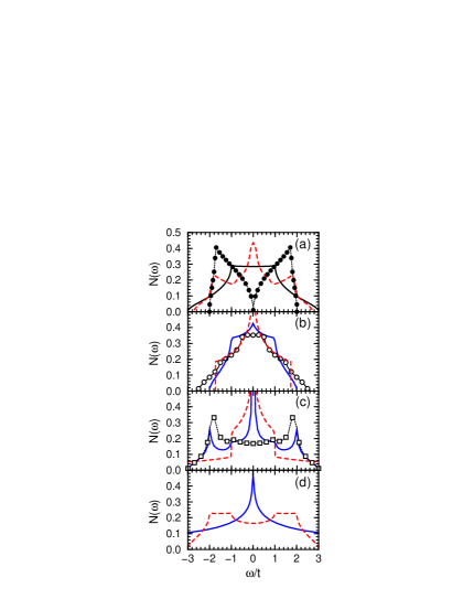
Figure 2: (Color online) Density of states $N(\omega)$ at $\gamma=1$ (in units of $t=1$) for different orbital ordered phases: (a) complex orbital order: uniform FO+ [degenerate with $A$-AO$\pm$] (solid line), $G$-AO$\pm$ (filled circles), and $C$-AO$\pm$ (dashed line); (b) alternating real orbital order in $G$-type phases: $G$-AO$sa$ (solid line) [the same density of states is obtained for $C$-AO$sa$ phase], $G$-AO$xz$ (dashed line), and $G$-AO$ab$ (circles); (c) alternating real orbital order in selected $C$- and $A$-type phases: $C$-AO$xz$ (solid line), $A$-AO$xz$ (dashed line), and $A$-AO$sa$ (squares); (d) real uniform orbital order FO$x$ (solid line) and FO$z$ (dashed line).

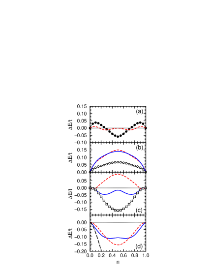
Figure 3: (Color online) Kinetic energy gain (loss) $\Delta E/t$ with respect to FO+ phase [reference zero energy given by horizontal dotted lines], as a function of electron filling $n$ for various orbital ordered phases (at $U=\infty$): (a) complex orbital order: $G$-AO$\pm$ (filled circles), and $C$-AO$\pm$ (dashed line); (b) alternating real orbital order in $G$-type phases: $G$-AO$sa$ (solid line) [degenerate with $C$-AO$sa$ phase], $G$-AO$xz$ (dashed line), and $G$-AO$ab$ (circles); (c) alternating real orbital order in selected $C$- and $A$-type phases: $C$-AO$xz$ (solid line), $A$-AO$xz$ (dashed line), and $A$-AO$sa$ (squares); (d) uniform real orbital order FO$x$ (solid line) and FO$z$ (dashed line). The long-dashed line in (d) shows the kinetic energy for noninteracting electrons in the $e_{g}$ band (disordered phase at $U=0$).

The other two orbital-ordered complex states break explicitly cubic symmetry: the $A$-type and $C$-type AO$\pm$ states. In the $A$-AO$\pm$ state layers of $|+\rangle$ and $|-\rangle$ orbitals alternate in the $c$ direction, resulting in the dispersion

$$\hskip-34.14322pt\varepsilon_{U=\infty,\pm}^{A-{\rm AO\pm}}({\bf k})=\frac{1}{3}t\big{[}(2\pm\gamma)A_{\bf k}-2(1\mp\gamma)C_{\bf k}\big{]}$$

$$\hskip 17.07182pt=t\big{(}\cos k_{a}+\cos k_{b}\pm\gamma\cos k_{c}\big{)}.$$ (43)

This dispersion is qualitatively equivalent to that of the FO+ state, and thus the densities of states of the FO+ and $A$-AO$\pm$ phases are the same. The reason is that replacing in the $c$-direction every second $|+\rangle$ orbital by a $|-\rangle$ orbital does not affect the hopping parameter along $c$, and so the resulting doubling of the unit cell only halves the Brillouin zone without changing the dispersion. In the $C$-AO$\pm$ state instead columns of $|+\rangle$ and $|-\rangle$ orbitals alternate in the $(a,b)$ planes, and one finds

$$\varepsilon_{U=\infty,\pm}^{C-{\rm AO\pm}}({\bf k}) = \frac{1}{3}t\Big{\{}A_{\bf k}+2C_{\bf k}\pm\gamma\Big{[}9D_{\bf k}^{2}+(A_{\bf k}-C_{\bf k})^{2}\Big{]}\Big{\}}$$ (44)

$$\hskip-71.13188pt=t\big{[}\cos k_{c}\pm\gamma\big{(}\cos^{2}k_{a}\!+\!\cos^{2}k_{b}-\cos k_{a}\cos k_{b}\big{)}^{1/2}\big{]}.$$

In contrast to the FO+, $G$-AO$\pm$ and $A$-AO$\pm$ phases, the $C$-AO$\pm$ phase is not cubic symmetric.

The densities of states of the complex states show a gradual crossover with increasing alternating orbital character from the full bandwidth of $6t$ for the FO+ and $A$-AO$\pm$ phases, obtained also at $U=0$ both for the spin problem and for the $e_{g}$ band (Fig. 1), to a narrower bandwidth of $2(1+\sqrt{3})t$ for the $C$-AO$\pm$ phase, and finally to a bandwidth of $4t$ for the $G$-AO$\pm$ phase. It is remarkable that, upon going from the FO+ phase to the $A$-AO$\pm$ phase, the change from uniform to alternating orbital order along only one cubic direction does not modify the density of states, while the density of states changes its shape completely upon going to the $G$-AO$\pm$ phase, with a large spectral weight accumulated now close to the band edges, resulting in a quite peculiar density of states with large maxima close to $|\omega|\simeq 2\gamma t$, separated by a minimum with $N(0)=0$ at $\omega=0$ [Fig. 2(a)]. The density of states for the $C$-AO$\pm$ phase has a width of $2(1+\sqrt{3})t$, and represents an intermediate case, having some features in common with that of the $G$-AO$\pm$ phase.

III.2 Densities of states and kinetic energies in orbital ordered states

It is worthwile to consider next the densities of states of various orbital ordered states in a little more detail (see Fig. 2), and investigate their consequences for the kinetic energy (Fig. 3). Focusing first on the bandwidth, we note that for any FO state this takes the maximum attainable value $6t$. This result is not limited to the FO states considered explicitly above, i.e., the complex FO+ and the real FO$z$ and FO$x$ states, for which it was already pointed out by Van den Brink and Khomskii,Bri01 but holds in general, i.e., for arbitrary $\psi$ and $\theta$, as readily shown from Eq. (17). Moreover, the result is independent of $\gamma$ and so holds both in the orbital case and in the spin case.

By contrast, in any $G$-type AO state the bandwidth is smaller than $6t$ [see Fig. 2(b)], and depends on $\gamma$. In particular, in any $G$-type “antiferro” state (with ${\bm{T}}_{A}=-{\bm{T}}_{B}$, so $\psi_{B}=\pi-\psi_{A}$ and $\theta_{B}=\theta_{A}-\pi$), such as the complex $G$-AO$\pm$ state or the real $G$-AO$xz$ and $G$-AO$sa$ states considered above, the width is proportional to $\gamma$ (viz. $4\gamma t$, $2\sqrt{3}\gamma t$, and $4\gamma t$, respectively for those three) as follows from Eq. (25). In such a state the bandwidth therefore, correctly, collapses to zero in the spin case ($\gamma=0$) where hopping is completely suppressed by the AF spin order.noteDE The important point to note here is that at finite $\gamma$, and so in particular in the genuine orbital case, the bandwidth even of an “antiferro” state is finite though smaller than that of the FO states. Thus, while in the spin case the kinetic energy of carriers is fully lost when going from FM to Néel-type AF order, this is not so for the analogous FO to $G$-type AO transition in the orbital case.

One might still be tempted to believe that, as familiar from the spin case, also in the orbital case FO order is most favorable for lowering the kinetic energy of charge carriers, simply because this gives the largest bandwidth. However, the situation is not that simple, not only because there are several inequivalent FO states with different densities of states which have nevertheless the same bandwidth, but also because some $A$-AO and $C$-AO phases have again the same bandwidth, and so one really has to consider the details of the density of states in each case. This is demonstrated in Fig. 3, which shows the kinetic energy gain $\Delta E$ with respect to the complex FO+ state as a function of electron filling $n$ for various FO and AO states with (complex or real) orbital order, obtained by straightforward integration of the respective density of states. Indeed, at small electron filling $n$, and also at small doping $x=1-n$, $\Delta E$ is lower for the (FO, $A$-AO and $C$-AO) states with full bandwidth $6t$ than for any state with a narrower density of states, in particular for the $G$-type AO states of Fig. 3(b), because the first doped holes enter in the former case with an energy $\sim-3t$ close to the band edge, while the lowest accessible energy is higher in all $G$-AO states. Note that the orbital order observed in LaMnO₃ is close to that of the $C$-AO$sa$ phase,noteMang and this phase has the same density of states as the $G$-AO$sa$ phase [see Fig. 2(b)], and thus has a rather unfavourable kinetic energy [Fig. 3(b)]. This demonstrates that both an interplay between spin and orbital order due to the SE interactions at finite $U$, and the JT interactions between orbitals on neighboring sites, induced by the coupling to the lattice, play an important role in real materials and stabilize the orbital order observed in undoped LaMnO₃.Fei99 ; Feh04

Among the states with AO order of real orbitals, but FO order along one or two cubic directions, we identified three phases, $C$-AO$xz$, $A$-AO$xz$, and $A$-AO$sa$, which have lower energies than the FO+ phase close to $n=0$ and $n=1$ [Fig. 3(c)]. All of them have the full bandwidth $6t$ [Fig. 2(c)], but a finite density of states at $\omega=-3t$ gives the $A$-AO$xz$ phase the lowest energy of these phases at very low $n$ or $x$. At somewhat higher filling $n\sim 0.07$ (doping $x\sim 0.07$) the other two phases take over, and are in fact more stable than the FO+ phase in the entire regime of $n$. This follows from the large densities of states of these phases at $|\omega|\simeq 2t$. In contrast, the $A$-AO$xz$ phase with a large spectral weight close to $\omega=0$ has a higher energy than the FO+ phase in a broad range of electron filling $0.11<n<0.89$.

The above discussion shows that at finite but still rather modest electron filling or doping, the overall shape of the density of states becomes more important, and the states with large density of states near the band edges could be favored a priori, even in cases when the bandwidth is smaller that $6t$. An interesting example here is the complex “antiferro” $G$-AO$\pm$ state, with its energy falling below that of the complex FO+ state for $n>0.27$ or $x>0.27$ [Fig. 3(a)], because of the large number of states available in the $G$-AO$\pm$ state just close to the band edges at $|\omega|=2t$, whereas in the FO+ state the energy of available electron states, though initially $-3t$, rises rapidly with increasing doping [Fig. 2(a)]. However, in reality the transition from FO+ to $G$-AO$\pm$ state does not happen, as the real FO (FO$z$ and FO$x$) states have even lower kinetic energy throughout than both complex states. This can be ascribed to the lower-dimensional nature of their dispersion and the resulting different location of the Van Hove singularities, which [compare Fig. 2(d)] enhances the density of states near the band edges at $\pm 3t$ and at the band center for the 2D FO$x$ state, and in the intermediate range $t\lesssim|\omega|\lesssim 2t$ for the quasi-1D FO$z$ state. As a result, at small filling (doping) the kinetic energy gain $\Delta E$ is the lowest one for the FO$x$ state, while at larger filling $n\gtrsim 0.30$ (doping $x\gtrsim 0.30$), the FO$z$ state takes over. However, in this regime of electron filling the energy gain $\Delta E$ for the $A$-AO$sa$ phase is lower by a few percent, and the two phases may be considered as practically degenerate.

For comparison and later reference we have included in Fig. 3 also the kinetic energy for the uncorrelated $e_{g}$ band (the correlated OL phase is analyzed in Sec. V). Of course, at $U=0$ any kind of orbital order is absent and one finds by far the lowest kinetic energy for the disordered $e_{g}$ orbitals. The $e_{g}$ bands have then the dispersion given by

$$\varepsilon_{U=0,\pm}({\bf k})=-t(A_{\bf k}\pm\gamma B_{\bf k}).$$ (45)

Remarkably, these bands at $U=0$ represent formally a superposition of the FO+ and $G$-AO$\pm$ bands at $U=\infty$,

$$\varepsilon_{U=0,\pm}({\bf k})=\varepsilon_{U=\infty}^{\rm FO+}({\bf k})+\varepsilon_{U=\infty,\pm}^{G-{\rm AO\pm}}({\bf k}).$$ (46)

and so naturally also show full cubic symmetry and a bandwidth equal to $6t$ [Fig. 1(d)]. One notes that, because both pseudospin-conserving and non-pseudospin-conserving hopping channels fully contribute here, considerably more kinetic energy can be gained than in any of the orbital-ordered states. In particular, as Fig. 1(d) shows, there is a large density of states at and near the band edges, and thus $\Delta E$ is the lowest in this disordered state already at small electron filling $n$, and then remains so throughout. Of course, this large kinetic energy gain will be partly lost for large $U$ near $n=1$, where at least one hopping channel gets partially suppressed by electron correlations. However, the result here indicates that the tendency towards the OL state with disordered $e_{g}$ orbitals is particularly pronounced. We shall come back to this point, presenting more evidence in favor of the correlated OL phase, in Sec. V.

IV Hartree-Fock approximation

IV.1 Instabilities towards orbital order

We turn now to the orbital Hubbard model (9) with finite $U$, where it is to be expected that polarization, when it occurs, need not be complete but can be partial, as in the spin case. Also, the existence of orbital ordered states will in general require a sufficiently large $U/t$. Which instabilities towards orbital ordering occur and at what value of $U/t$ can be investigated either by considering the corresponding susceptibilities, e.g. in random phase approximation,Shi00 or by comparing the energies determined in the HF approximation.Bri01 If various ordered states are possible, one needs to calculate their energy (or free energy at finite temperature) to determine which one is actually realized.

In the absence of SU(2) symmetry it is not sufficient to decouple the interaction term in Eq. (9) in the familiar mean-field way, $n_{i+}n_{i-}\simeq(\langle n_{i+}\rangle n_{i-}+n_{i+}\langle n_{i-}\rangle-\langle n_{i+}\rangle\langle n_{i-}\rangle)$, but one needs instead the general HF decoupling,

$$n_{i+}n_{i-}\simeq\Big{(}\langle n_{i+}\rangle n_{i-}+n_{i+}\langle n_{i-}\rangle-\langle n_{i+}\rangle\langle n_{i-}\rangle\Big{)}-\left(\langle T_{i}^{+}\rangle c_{i-}^{\dagger}c_{i+}+c_{i+}^{\dagger}c_{i-}\langle T_{i}^{-}\rangle-\langle T_{i}^{+}\rangle\langle T_{i}^{-}\rangle\right).$$ (47)

In the FO case, i.e., when one assumes a single three-component order parameter, $T_{z}=\langle T_{i}^{z}\rangle$, $T_{+}=\langle T_{i}^{+}\rangle$, $T_{-}=\langle T_{i}^{-}\rangle$, one obtains upon Fourier transformation the HF Hamiltonian

$$H_{\rm HF}^{\rm FO} = \sum_{\bf k}\left(c_{{\bf k}+}^{\dagger}\;c_{{\bf k}-}^{\dagger}\right)\left(\begin{array}[]{cc}\textstyle{\frac{1}{2}}Un-UT_{z}-tA_{\bf k}&-UT_{-}-\gamma tP_{\bf k}^{\ast}\\[5.69046pt] -UT_{+}-\gamma tP_{\bf k}&\textstyle{\frac{1}{2}}Un+UT_{z}-tA_{\bf k}\end{array}\right)\left(\begin{array}[]{c}c_{{\bf k}+}\\[5.69046pt] c_{{\bf k}-}\end{array}\right)$$ (53)

$$-\textstyle{\frac{1}{4}}Un^{2}+U(T_{z}^{2}+T_{+}T_{-}),$$

with $P_{\bf k}$ given by Eq. (21). The eigenvalues are (with $T_{+}=Te^{i\theta}$, $T_{-}=Te^{-i\theta}$, so that $T_{+}T_{-}=T^{2}=T_{x}^{2}+T_{y}^{2}$)

$$\varepsilon_{\pm}^{\rm FO}({\bf k})=-tA_{\bf k}+U\big{(}\textstyle{\frac{1}{2}}n\pm\hat{E}_{\bf k}\big{)},$$ (54)

where

$$\hat{E}_{\bf k}=\Big{[}T^{2}+T_{z}^{2}+2\frac{\gamma t}{U}T\big{(}\cos\theta C_{\bf k}+\sin\theta D_{\bf k}\big{)}+\Big{(}\frac{\gamma t}{U}\Big{)}^{2}B_{\bf k}^{2}\Big{]}^{1/2},$$ (55)

and the HF groundstate energy per site is then given by

$$E_{\rm HF}^{\rm FO}=\frac{1}{N}\sum_{\bf k}\Big{[}n_{-}({\bf k})\varepsilon_{-}^{\rm FO}({\bf k})+n_{+}({\bf k})\varepsilon_{+}^{\rm FO}({\bf k})\Big{]}-\frac{1}{4}Un^{2}+U\big{(}T^{2}+T_{z}^{2}\big{)},$$ (56)

where $n_{-}({\bf k})$ [$n_{+}({\bf k})$] is the occupation number of the lower (upper) band. For large $U$ ($\gtrsim 6t$) a gap opens, and so for less than half-filling only the lower band is occupied. Setting the derivatives of $E_{\rm HF}^{\rm FO}$ with respect to $n$, $T_{z}$, $T$, and $\theta$ equal to zero then yields the self-consistency equations

$$\hskip-19.91684ptn = \frac{1}{N}\sum_{\bf k}n_{-}({\bf k}),$$ (57)

$$\hskip-19.91684ptT_{z} = \frac{1}{2}\frac{1}{N}\sum_{\bf k}n_{-}({\bf k})\frac{T_{z}}{\hat{E}_{\bf k}},$$ (58)

$$\hskip-19.91684ptT = \frac{1}{2}\frac{1}{N}\sum_{\bf k}n_{-}({\bf k})\frac{T+\frac{\gamma t}{U}\big{(}\cos\theta\,C_{\bf k}+\sin\theta\,D_{\bf k}\big{)}}{\hat{E}_{\bf k}},$$ (59)

$$\hskip-19.91684pt0 = \frac{1}{2N}\sum_{\bf k}n_{-}({\bf k})\frac{T\big{(}\sin\theta\,C_{\bf k}-\cos\theta\,D_{\bf k}\big{)}}{\hat{E}_{\bf k}}.$$ (60)

While Eq. (57) is trivially satisfied in the sense that it simply fixes the Fermi level for given filling $n$, two general conclusions can be proven from the remaining three equations. Firstly, it follows from Eq. (60), because of the dependence of $\hat{E}_{\bf k}$ on $C_{\bf k}$ and $D_{\bf k}$ [see Eq. (55)] and the explicit form of the latter two functions [see Eqs. (19) and (20)], that for nonzero $T$ the azimuth $\theta$ must equal either $0$ (or equivalently $+2\pi/3$ or $-2\pi/3$) or $\pi$ (or equivalently $-\pi/3$ or $+\pi/3$), i.e. the projection of the order parameter on the ‘real’ equatorial plane has to be along one of the cubic directions. Secondly, it follows that both a purely complex state (i.e., $T=0$, $T_{z}\neq 0$) and a purely real state (i.e., $T_{z}=0$, $T\neq 0$) are permissible states, in the sense that $T_{z}=0$ is a self-consistent solution of Eq. (58) and alternatively $T=0$ is one of Eq. (59). We remark that both these properties of the possible states need not be postulated or assumed but are proven here from the HF self-consistency equations.

As $C$-type and $A$-type AO phases would give qualitatively similar results, we will consider from now on only $G$-type AO phases, and denote them for brevity by “AO” instead of by “$G$-AO”. So we assume independent three-component order parameters on interlacing sublattices A and B, $T_{z}^{\rm A}=\langle T_{i}^{z}\rangle_{\rm A}$, $T_{z}^{\rm B}=\langle T_{i}^{z}\rangle_{\rm B}$, etc. Then the HF Hamiltonian is

$$H_{\rm HF}^{\rm AO} = \sum_{\bf k}\left(\begin{array}[]{c}c_{{\rm A},{\bf k}+}^{\dagger}\\ c_{{\rm A},{\bf k}-}^{\dagger}\\ c_{{\rm B},{\bf k}+}^{\dagger}\\ c_{{\rm B},{\bf k}-}^{\dagger}\end{array}\right)^{\!\!\rm T}\left(\begin{array}[]{cccc}\textstyle{\frac{1}{2}}Un-UT_{z}^{\rm A}&-UT_{-}^{\rm A}&-tA_{\bf k}&-\gamma tP_{\bf k}^{\ast}\\[5.69046pt] -UT_{+}^{\rm A}&\textstyle{\frac{1}{2}}Un+UT_{z}^{\rm A}&-\gamma tP_{\bf k}&-tA_{\bf k}\\[5.69046pt] -tA_{\bf k}&-\gamma tP_{\bf k}^{\ast}&\textstyle{\frac{1}{2}}Un-UT_{z}^{\rm B}&-UT_{-}^{\rm B}\\[5.69046pt] -\gamma tP_{\bf k}&-tA_{\bf k}&-UT_{+}^{\rm B}&\textstyle{\frac{1}{2}}Un+UT_{z}^{\rm B}\end{array}\right)\left(\begin{array}[]{c}c_{{\rm A},{\bf k}+}\\[5.69046pt] c_{{\rm A},{\bf k}-}\\[5.69046pt] c_{{\rm B},{\bf k}+}\\[5.69046pt] c_{{\rm B},{\bf k}-}\end{array}\right)$$ (74)

$$-\textstyle{\frac{1}{4}}Un^{2}+\textstyle{\frac{1}{2}}U\big{[}\big{(}T_{z}^{\rm A}\big{)}^{2}+T_{+}^{\rm A}T_{-}^{\rm A}+\big{(}T_{z}^{\rm B}\big{)}^{2}+T_{+}^{\rm B}T_{-}^{\rm B}\big{]}.$$

Like above, the HF groundstate energy per site is then formally given (with $T_{+}^{\rm A}=T^{\rm A}e^{i\theta_{\rm A}}$, etc.) by

$$E_{\rm HF}^{\rm AO}=\frac{1}{N}\sum_{\beta=1}^{4}\sum_{\bf k}n_{\beta}({\bf k})\varepsilon_{\beta}^{\rm AO}({\bf k})-\textstyle{\frac{1}{4}}Un^{2}+\textstyle{\frac{1}{2}}U\big{[}\big{(}T^{\rm A}\big{)}^{2}+\big{(}T_{z}^{\rm A}\big{)}^{2}+\big{(}T^{\rm B}\big{)}^{2}+\big{(}T_{z}^{\rm B}\big{)}^{2}\big{]},$$ (75)

where the sum on $\beta$ is over the four bands and that on ${\bf k}$ is over the reduced Brillouin zone. However, as the $4\times 4$ matrix in Eq. (75) cannot be diagonalized analytically in the general case (i.e. for arbitrary order parameters), no further progress can be made like in the FO case. In particular one cannot strictly prove that purely real or purely complex states are permissible solutions.

Yet this still seems likely, and if one makes this assumption, then for the case of the complex (AO$c$) state, i.e. with $T^{\rm A}=T^{\rm B}=0$, the $4\times 4$ matrix simplifies enough to obtain explicit expressions for the band dispersions,

$$\varepsilon_{\beta}^{\rm AOc}({\bf k})=+U\big{(}\textstyle{\frac{1}{2}}n\pm\hat{F}_{1,{\bf k}}\pm\hat{F}_{2,{\bf k}}\big{)},$$ (76)

where

$$\hat{F}_{1,{\bf k}} = \Big{[}\Big{(}\frac{T_{z}^{\rm A}+T_{z}^{\rm B}}{2}\Big{)}^{2}+\Big{(}\frac{\gamma t}{U}\Big{)}^{2}B_{\bf k}^{2}\Big{]}^{1/2},$$ (77)

$$\hat{F}_{2,{\bf k}} = \Big{[}\Big{(}\frac{T_{z}^{\rm A}-T_{z}^{\rm B}}{2}\Big{)}^{2}+\Big{(}\frac{t}{U}\Big{)}^{2}A_{\bf k}^{2}\Big{]}^{1/2}.$$ (78)

Setting the derivatives of $E_{\rm HF}^{\rm AOc}$ with respect to $n$, $T_{z}^{\rm A}$ and $T_{z}^{\rm B}$ to zero yields again HF self-consistency equations. From these one easily proves that $T_{z}^{\rm A}=-T_{z}^{\rm B}$, i.e. that the stable complex state is actually the AO$\pm$ state.

For the case of a real (AOr) state, i.e., with $T_{z}^{\rm A}=T_{z}^{\rm B}=0$, an analytic solution is also possible, but this is so unwieldy as to be impractical. However, if one further assumes that $T^{\rm A}=T^{\rm B}\equiv T$ one can derive the approximate expressions

$$\varepsilon_{\beta}^{\rm AOr}({\bf k}) = \pm t\big{[}A_{\bf k}\cos\theta_{-}+\gamma\big{(}C_{\bf k}\cos\theta_{+}+D_{\bf k}\sin\theta_{+}\big{)}\big{]}$$ (79)

$$+ U\big{(}\textstyle{\frac{1}{2}}n\pm\hat{G}_{\bf k}\big{)},$$

where

$$\hat{G}_{\bf k} = \Big{[}T^{2}+\Big{(}\frac{t}{U}\Big{)}^{2}\big{\{}A_{\bf k}^{2}\sin^{2}\theta_{-}$$ (80)

$$\!+\gamma^{2}\big{(}C_{\bf k}\sin\theta_{+}-D_{\bf k}\cos\theta_{+}\big{)}^{2}\big{\}}\Big{]}^{1/2},$$

valid in the large $U$ limit ($U/t\gg 1$), and again obtain analytic self-consistency equations by taking the derivatives of $E^{\rm AOr}$ with respect to $n$, $T$, $\theta_{+}$, and $\theta_{-}$. From the latter two one can now prove the following. First, that $\theta_{+}=0$, i.e., $\theta_{\rm A}=-\theta_{\rm B}$, so the pseudospin vectors on the two sublattices are mirror images of one another with respect to the cubic direction $\theta=0$ (or the equivalent ones $\theta=\pm 2\pi/3$). Second, that $\cos\theta_{-}\simeq-(U/3t)x$ for $x\ll t/U$, i.e., $\theta_{\rm A}\simeq\pi/2+(U/3t)x$, so that at zero doping the stable solution is the AO$sa$ state, and with increasing doping the pseudospin vectors tilt slightly away from the cubic direction, making the solution gradually resemble more the AO$ab$ state.noteAOreal

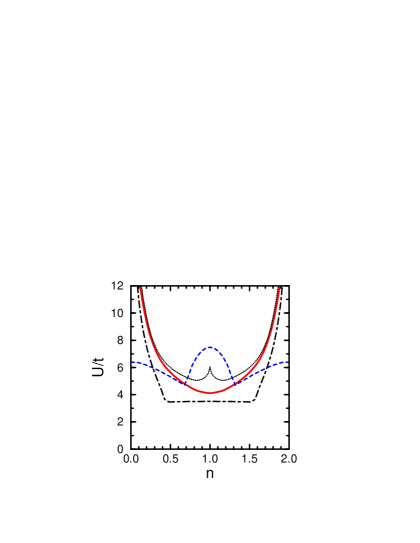
Figure 4: (Color online) Stoner instability towards FO+ partly polarized states (full line) as a function of band filling $n$ in the orbital Hubbard model ($\gamma=1$), and the inverse of the $e_{g}$ density of states of Fig. 1(d) (dotted line); full polarization occurs only in the limit $U=\infty$. For the spin model ($\gamma=0$), the corresponding Stoner instability (dashed-dotted line) is given by the inverse of the density of states shown in Fig. 1(a), while saturated FM states occur above the dashed line.

As an example of the HF instability at intermediate $U$ we have investigated how the complex FO+ (or the equivalent FO$-$) state develops when $U$ increases, using Eqs. (53) and (56). First, at $\gamma=0$ one recovers the Stoner criterion $U_{o}N(E_{F})=1$ for the onset of the FM order with increasing $U$, with the FM saturated states becoming stable at still larger but finite value of $U$ (Fig. 4). By contrast, in the orbital model at $\gamma=1$ the instability is qualitatively different, and the FO+ (FO$-$) state appears as a global property of the band rather than as an instability at the Fermi surface. The instability occurs at higher values of $U$ for any filling than in the spin case — actually the value of the critical $U$ is very close to that giving full magnetic polarization in the spin case.

Here, unlike in the spin case, the FO order implies that the electronic bands are changed — they develop an additional splitting above a critical value of $U$, which modifies the shape of the bands and leads to a finite order parameter $T_{z}=\langle T_{i}^{z}\rangle\neq 0$. This mechanism of the instability resembles that known in the spin case for the onset of antiferromagnetism. The critical value of $U$ above which weak order appears has therefore no relation to the actual shape of the density of states (see Fig. 4).

We decided not to investigate the phase diagram of the orbital Hubbard model in the HF approximation in detail. Instead, we concentrate first on the qualitatively novel aspects of various possible ordered states in the regime of large $U$, where, as we will see, the contrast with the spin case manifests itself in the most transparent way. Using these results, we will then comment of the HF phase diagrams analyzed in detail by several groups,Shi00 ; Bri01 ; Mae00 in Sec. IV.4.

IV.2 Superexchange in the complex orbital states

We have already seen that the analysis of the orbital-ordered states simplifies when the splitting of the quasiparticle bands $\propto UT_{z}$ or $\propto UT$ is sufficiently large that it opens up a gap and only the lower band (lowest two bands for AO order) is (are) partly occupied when $n\leq 1$. It is then straightforward to calculate the energy and the order parameter by summing over the occupied states.

Consider first the ordered states with complex orbitals. In the case of the FO+ state the equation for the order parameter, from Eqs. (59) and (55), takes the simple form (because only $T_{z}\neq 0$, while $T=0$):

$$T_{z} = \frac{1}{2}\frac{1}{N}\sum_{\bf k}\frac{n_{-}({\bf k})}{E_{\bf k}},$$ (81)

$$E_{\bf k} = \Big{[}1+\Big{(}\frac{\gamma t}{UT_{z}}\Big{)}^{2}B_{\bf k}^{2}\Big{]}^{1/2}.$$ (82)

Equation (82) shows explicitly that, unlike in the spin case, $T_{z}=n/2$ only at $U=\infty$, basically because the saturated FO+ state is not an eigenstate of the orbital Hubbard model given by Eq. (9). Thus the FO+ state is again seen to resemble the AF phase in the spin model.

Similarly, in the AO$\pm$ phase for large enough $U$ the order parameter is given by

$$T_{z} = \frac{1}{2}\frac{1}{N}\sum_{\bf k}\frac{n_{1}({\bf k})+n_{2}({\bf k})}{F_{\bf k}},$$ (83)

$$F_{\bf k} = \Big{[}1+\Big{(}\frac{t}{UT_{z}}\Big{)}^{2}A_{\bf k}^{2}\Big{]}^{1/2},$$ (84)

rather similar to the FO+ case (82), but with the interchange $A_{\bf k}\leftrightarrow\gamma B_{\bf k}$. The reason is readily recognized from Eq. (9): for FO+ order, the diagonal hopping $\propto c_{i\pm}^{\dagger}c_{j\pm}$ that gives $A_{\bf k}$, is order-preserving, while the off-diagonal terms $\propto c_{i\pm}^{\dagger}c_{j\mp}$ that produce $B_{\bf k}$ are order-perturbing and reduce $T_{z}$. For AO$\pm$ order this is reversed: the off-diagonal hopping $\propto\gamma$ that gives $B_{\bf k}$ is compatible with the order, while the diagonal one that gives $A_{\bf k}$ disturbs it.

The similarity between the FO+ and AO$\pm$ states at $\gamma\simeq 1$ becomes even more transparent at large $U$ (i.e. $\gg t$), where near half-filling (i.e. for small $x=1-n>0$), upon expansion up to first order in $t/U$,

$$T_{z}^{{\rm FO}+} = \frac{1}{2}\Big{\{}(1-x)-\frac{3\gamma^{2}}{(1-x)^{2}}\Big{(}\frac{t}{U}\Big{)}^{2}\Big{\}},$$ (85)

$$T_{z}^{{\rm AO}\pm} = \frac{1}{2}\Big{\{}(1-x)-\frac{3-2x}{(1-x)^{2}}\Big{(}\frac{t}{U}\Big{)}^{2}\Big{\}}.$$ (86)

Note that a SE contribution $\propto(\gamma t)^{2}/U$ appears also in the FO+ state, because the off-diagonal hopping permits virtual charge fluctuations. This result is again qualitatively different from the spin case, where the SE contributes only in the AF states, and so destabilizes uniform FM spin order. In the genuine orbital case ($\gamma=1$) the reduction of the order parameter by SE is the same for FO+ and AO$\pm$ at $x=0$, but at $x\gtrsim 0$ it is slightly larger for the FO+ phase. The corresponding expressions for the energy, up to second order in $t/U$, become

$$\hskip-34.14322ptE^{{\rm FO}+}=-t\frac{1}{N}\sum_{\bf k}n_{-}({\bf k})A_{\bf k}-\frac{3\gamma^{2}}{2(1-x)}\;\frac{t^{2}}{U},$$ (87)

$$\hskip-34.14322ptE^{{\rm AO}\pm}=-\gamma t\frac{1}{N}\sum_{\bf k}\big{[}n_{1}({\bf k})-n_{2}({\bf k})\big{]}B_{\bf k}$$

$$\hskip 5.69046pt-\frac{3-2x}{2(1-x)}\;\frac{t^{2}}{U}.$$ (88)

Both are seen to be composed of the $U=\infty$ kinetic energy (compare Eqs. (41) and (42) for the dispersions) and a (negative) SE energy. Surprisingly, near half-filling the energy per site of the FO phase is lower than that of the AO phase at any value of $U$, not only because the FO phase gains more kinetic energy $\propto-3tx$ than the AO phase $\propto-2tx$, but also because it has lower SE energy. Instead, AO$\pm$ order yields lower energy at larger doping $x\gtrsim 0.27$ as a consequence of its peculiar density of states [Fig. 2(a)].Shi00 ; Mae00 Note that this is opposite to the spin case ($\gamma=0$), where the Néel (AF) state has lower energy near $n=1$ and the FM state takes over only above a critical doping $x_{c}\simeq t/2U$.

We emphasize that we have compared as yet only the two complex states with one another, with the express purpose of contrasting the behavior of these orbital states with that of the corresponding spin states. To establish what the most stable orbital-ordered state is, we still have to consider the real states.

IV.3 Superexchange in the real orbital states

The results obtained for the ordered phases with real orbitals are qualitatively similar. We focus here on the representative cases of the FO$x$, the FO$z$, and the ($G$-type) AO$sa$ states, which we have shown in Section IV to be solutions of the HF equations. Note that the AO$sa$ phase is representative for $G$-type AO order. For simplicity we ignore here the small higher order correction to the equations below,noteAOxpmz which occur when the actual occupied orbitals deviate from those of the AO$sa$ state towards those pertaining to the AO$ab$ state as discussed above.

At large $U/t$ one finds near half-filling for the order parameters

$$\hskip-39.83368ptT^{{\rm FO}x(z)}\!=\!\frac{1}{2}\Big{\{}(1-x)-\frac{3\gamma^{2}}{2(1-x)^{2}}\Big{(}\frac{t}{U}\Big{)}^{2}\Big{\}},$$ (89)

$$\hskip-34.14322ptT^{{\rm AO}sa}\!=\!\frac{1}{2}\Big{\{}(1-x)-\frac{6-4x+3\gamma^{2}}{2(1-x)^{2}}\Big{(}\frac{t}{U}\Big{)}^{2}\Big{\}}.$$ (90)

The corresponding energies in these ordered phases are

$$E^{{\rm FO}x} = -t\frac{1}{N}\sum_{\bf k}n_{-}({\bf k})\big{(}A_{\bf k}-\gamma C_{\bf k}\big{)}-\frac{3\gamma^{2}}{4(1-x)}\;\frac{t^{2}}{U},$$ (91)

$$E^{{\rm FO}z} = -t\frac{1}{N}\sum_{\bf k}n_{-}({\bf k})\big{(}A_{\bf k}+\gamma C_{\bf k}\big{)}-\frac{3\gamma^{2}}{4(1-x)}\;\frac{t^{2}}{U},$$ (92)

$$E^{{\rm AO}sa} = -t\frac{1}{N}\sum_{\bf k}\big{[}(n_{1}({\bf k})-n_{2}({\bf k})\big{]}\gamma C_{\bf k}-\frac{6-4x+3\gamma^{2}}{4(1-x)}\;\frac{t^{2}}{U}.$$ (93)

Unlike the complex states, the real states are seen not to be degenerate in the undoped case $x=0$. The AO$sa$ state has the lowest energy here, even though the SE contributes also in the FO states. However, we find the same qualitative difference with the familiar AF and FM states for spin order as we found for the complex orbital states — again the SE contributes both in FO and in AO states.

Finally, we remark that the SE contributes also in any other phase, either with mixed FO and AO order (e.g. in the $C$-AO and $A$-AO phases of Sec. III), or in a disordered OL state. Depending on whether the occupied orbitals on a given bond are identical or not, virtual processes due to pseudospin non-conserving or pseudospin conserving hopping contribute, and we have verified that qualitatively similar results are then obtained to those presented in Eqs. (89-93) above. Such terms would play a role in the low-doping regime and would deserve a separate study in order to establish the phase diagram of weakly doped manganites. Note that in that regime also the spin-dependent SE plays a prominent role, and the present orbital Hubbard model (9), which implicitly assumes FM order, becomes insufficient to describe the physical properties of the real materials. On the other hand, the SE terms, being all $\propto t^{2}/U$, vanish in the limit of large $U$ which we consider in Sec. V, and hence they have no consequences for the stability of the OL phase at $U=\infty$.

IV.4 Qualitative understanding of the Hartree-Fock phase diagram

Finally, let us analyze the possible instabilities of the orbital Hubbard model (9) in the HF approximation. In the large $U$ limit relevant for such instabilities, the total energy consists of the kinetic energy at $U=\infty$, discussed in Sec. III.1, and a negative SE energy. While we do not intend to make a quantitative comparison between the various phases stable in the HF approximation, knowing that they are anyway destabilized by the correlation effects (see Sec. V), this now enables us to get a simple interpretation of the HF phase diagram of the genuine $e_{g}$ orbital model ($\gamma=1$),Shi00 ; Bri01 ; Mae00 ; She00 using the large $U$ expansion. These earlier HF studies have shown that at half-filling, and in the regime of small doping, for $U>6t$ the most stable state is the real ‘antiferro’ orbital state, with the orbitals close to those found in the AO$sa$ phase. In this regime the SE energy dominates, and indeed the largest energy gain is then given by Eq. (93). At increasing hole doping, however, the kinetic energy of holes moving in the FO$x$ background is much lower than that in the AO$sa$ phase (see Fig. 3), leading to a transition to ‘ferro’ orbital states when the difference between the SE terms $\propto t^{2}/U$ is overcome by the difference between the kinetic energies of these two phases. The region of the AO$sa$ phase in the phase diagram decreases when the SE gradually looses its importance with increasing $U$, as shown by the numerical result of Van den Brink and Khomskii.Bri01

At $U=\infty$ the FO$r$ order is found in the HF approximation at any doping $x>0$. However, at large but finite $U$ the SE is larger in the FO+ than in either FO$x$ or FO$z$ phase, while the difference in the kinetic energy is small [Fig. 3(d)], and thus the FO+ state is the first stable ‘ferro’ state at intermediate values of $8<U/t<12$ and $x\simeq 0.15$. However, when $x$ increases further, the kinetic energy difference between the FO$x$ and FO+ phase dominates, and the orbital order changes to FO$x$. As the SE energy of the two real FO$x$ and FO$z$ states [see Eqs. (91) and (92)] is the same, the difference in the kinetic energy gives a second transition from the FO$x$ to the FO$z$ phase with increasing $x$. At small and intermediate $U/t<12$ one finds eventually at $x\sim 0.5$ the AO$\pm$ phase,Bri01 which is stabilized in this regime by a combined effect of large SE energy gain and low kinetic energy (see Fig. 3) which follows from the peculiar density of states of this phase.

In a 2D model the phase diagram is quite different,Tha00 and is dominated by the generic tendency towards $x^{2}-y^{2}$ polarization within an $(a,b)$ plane.Mac99 The AO order is then followed by the FO$x$ phase above a critical doping, which decreases with increasing $U/t$. We note that the region of the FO$x$ phase is enlarged by the offdiagonal hopping terms $\propto\gamma t$,Tha00 in agreement with the above observation that these terms stabilize the FO phases at finite $U$ due to the respective SE energy contributions.

V Orbital liquid state

V.1 Kotliar-Ruckenstein slave boson representation

To understand further the essential differences between orbital and spin physics, we develop now an approximate description of the correlated OL disordered state. This is of crucial importance as the HF approximation permits only a comparison of ordered states with one another, and therefore does not allow to draw any conclusions concerning the stability of the orbital-ordered states with respect to disordered states. This is well known from spin models — for instance, the FM states in the 2D Hubbard model are stable only in a narrow range of doping $x<0.29$ near half-filling,vdL91 while the HF approximation predicts FM to be stable at any electron filling $n$.

We will argue below that indeed orbital (FO or AO) order is not robust at $\gamma=1$ and gets replaced by a disordered (OL) phase, if one goes beyond the HF approximation and includes electron correlation effects. As we have already seen, the orbital problem is richer than the spin case, as various ordered states are nonequivalent when the SU(2) symmetry is absent. Therefore, we shall consider only the limit of very strong correlations and investigate the stability of orbital order specifically in the $U=\infty$ limit, where the OL competes with fully saturated FO [see Eqs. (85) and (89)] and AO [see Eqs. (86) and (90] states.

In order to obtain a reliable variational method to calculate the correlation energy, we have followed the slave boson approach introduced by Kotliar and Ruckenstein Kot86 for the spin Hubbard model, and have adapted it to the orbital case. In this approach the Fock space is enlarged by the introduction of three auxiliary bosons at each site, one for each local configuration, viz. $b_{i+}$ and $b_{i-}$ associated with the single-occupancy configurations $|i+\rangle$ and $|i-\rangle$, and $e_{i}$ with the empty configuration $|i0\rangle$ (double occupancy is excluded at $U=\infty$). Then a physical fermion (electron) $c$ is represented by a pseudofermion $f$ and two accompanying bosons according to an expression like $c_{i\beta}^{\dagger}=f_{i\beta^{\prime}}^{\dagger}b_{i\beta}^{\dagger}e_{i}$, where the two bosons keep track of the change of the local configuration when an electron is added.Kot86 This construction, however, must preserve the cubic symmetry of the Hamiltonian (9), implying that it has to be gauge invariant with respect to those U(1) rotations in orbital space that correspond to a permutation of the cubic axes. The relevant rotation operator is, for arbitrary rotation angle $\theta$,

$$\hat{U}_{i}(\theta)=\exp\Big{(}-i\theta T_{i}^{z}\Big{)}.$$ (94)

The complex orbitals pick up just a phase factor under any rotation of this form, and the operators $\{c_{i+}^{\dagger},c_{i-}^{\dagger}\}$ transform as

$$\hat{U}_{i}(\theta)c_{i+}^{\dagger}\hat{U}_{i}^{\dagger}(\theta) = e^{-i\theta/2}c_{i+}^{\dagger},$$

$$\hat{U}_{i}(\theta)c_{i-}^{\dagger}\hat{U}_{i}^{\dagger}(\theta) = e^{+i\theta/2}c_{i-}^{\dagger}.$$ (95)

As already indicated in Section II, the orbital Hubbard Hamiltonian (9) is invariant under a uniform rotation at all sites, if the common rotation angle $\theta$ is one of the three cubic angles $-4\pi/3$, $+4\pi/3$, $0$, and if this is accompanied by a corresponding shift of the “gauge angles” $\chi_{\alpha}$ by $+2\pi/3$, $-2\pi/3$, $0$, respectively. Actually the diagonal hopping terms in (9) are invariant under the U(1) transformation (94) even for arbitrary $\theta$, as a consequence of the SU(2) symmetry of the spin Hubbard model, while the off-diagonal hopping terms pick up phase factors,

$$c_{i+}^{\dagger}c_{j-} \mapsto e^{-i\theta}c_{i+}^{\dagger}c_{j-},$$

$$c_{i-}^{\dagger}c_{j+} \mapsto e^{+i\theta}c_{i-}^{\dagger}c_{j+},$$ (96)

which get compensated by the shift of the $\chi_{\alpha}$ if $\theta$ is a cubic angle. As the three cubic-angle transformations amount to a forward and to a backward simultaneous cyclic permutation of axes and orbitals and to the identity, respectively, the invariance expresses the cubic symmetry of the Hamiltonian.

Therefore, we take the slave boson representation as

$$c_{i\pm}^{\dagger}=b_{i\pm}^{\dagger}f_{i\mp}^{\dagger}e_{i},$$ (97)

corresponding to a representation of the local states by

$$|i0\rangle = e_{i}^{\dagger}|{\rm vac}\rangle,$$

$$|i+\rangle=c_{i+}^{\dagger}|i0\rangle = b_{i+}^{\dagger}f_{i-}^{\dagger}|{\rm vac}\rangle,$$

$$|i-\rangle=c_{i-}^{\dagger}|i0\rangle = b_{i-}^{\dagger}f_{i+}^{\dagger}|{\rm vac}\rangle,$$ (98)

and we impose that the boson and pseudofermion operators transform under U(1) rotations noteU1 as

$$\hat{U}_{i}(\theta)\>e_{i}^{\dagger}\>\hat{U}_{i}^{\dagger}(\theta) = e_{i}^{\dagger},$$

$$\hat{U}_{i}(\theta)b_{i\pm}^{\dagger}\hat{U}_{i}^{\dagger}(\theta) = e^{\mp i\theta}\,b_{i\pm}^{\dagger},$$

$$\hat{U}_{i}(\theta)f_{i\pm}^{\dagger}\hat{U}_{i}^{\dagger}(\theta) = e^{\mp i\theta/2}f_{i\pm}^{\dagger}.$$ (99)

Note that the phase of the boson operators $b_{i\pm}^{\dagger}$ changes twice as fast as the phase of the pseudofermion operators $f_{i\pm}^{\dagger}$, i.e. the bosons have pseudospin $T=1$, while the (pseudo)fermions belong to $T=1/2$. This property guarantees that the U(1) rotation behavior of the electron operators, as given in Eqs. (95), is correctly reproduced by the transformation (97). Thus the present formulation is indeed gauge invariant and preserves the cubic symmetry of the orbital problem, like the SU(2)-invariant formulation introduced by Frésard and Wölfle preserves the full rotational symmetry for the spin system.Fre92 Clearly, the construction of a gauge invariant formulation is greatly facilitated by our use of the complex-orbital representation, but a similarly gauge invariant representation in terms of real operators can also be constructed, and is given in the Appendix.

The enlarged Fock space contains also unphysical states which must be eliminated by imposing constraints as in the original formulation by Kotliar and Ruckenstein,Kot86

$$b_{i+}^{\dagger}b_{i+}+b_{i-}^{\dagger}b_{i-}+e_{i}^{\dagger}e_{i} = 1,$$

$$b_{i+}^{\dagger}b_{i+}=f_{i-}^{\dagger}f_{i-},\hskip 14.22636ptb_{i-}^{\dagger}b_{i-} = f_{i+}^{\dagger}f_{i+},$$ (100)

and implemented by means of Lagrange multiplyers $\{\lambda_{i},\mu_{i+},\mu_{i-}\}$. The first constraint excludes double occupancy, the other two eliminate the unphysical singly-occupied states $b_{i+}^{\dagger}f_{i+}^{\dagger}|{\rm vac}\rangle$ and $b_{i-}^{\dagger}f_{i-}^{\dagger}|{\rm vac}\rangle$. The electron density and the $z$-component of the pseudospin can then be described at each site either by slave boson or by pseudofermion operators,

$$\hskip-31.2982ptn_{i}\!\equiv c_{i+}^{\dagger}c_{i+}+c_{i-}^{\dagger}c_{i-}$$

$$\hskip-20.48601pt=b_{i+}^{\dagger}b_{i+}+b_{i-}^{\dagger}b_{i-}=f_{i+}^{\dagger}f_{i+}+f_{i-}^{\dagger}f_{i-},$$ (101)

$$\hskip-34.14322ptT_{i}^{z}\!=\textstyle{\frac{1}{2}}(b_{i+}^{\dagger}b_{i+}\!-b_{i-}^{\dagger}b_{i-})=\textstyle{\frac{1}{2}}(f_{i-}^{\dagger}f_{i-}\!-f_{i+}^{\dagger}f_{i+}).$$ (102)

The other two components of the pseudospin operator can only be represented as

$$T_{i}^{+}=b_{i+}^{\dagger}b_{i-}f_{i-}^{\dagger}f_{i+},$$ (103)

$$T_{i}^{-}=b_{i-}^{\dagger}b_{i+}f_{i+}^{\dagger}f_{i-},$$ (104)

and cannot be reduced to expressions in terms of either slave bosons or pseudofermions alone.note-T+T-

As in the spin case one further has to renormalize the bosonic factor in Eq. (97) in order to recover, when a mean-field approximation is going to be made and the constraints are no longer rigorously obeyed, the correct unrenormalized hopping for the pseudofermions in the uncorrelated ($U=0$) limit. The renormalized boson factors take the form

$$z_{i\pm}^{\dagger}=\frac{b_{i\pm}^{\dagger}e_{i}}{\sqrt{(1-e_{i}^{\dagger}e_{i}-b_{i\mp}^{\dagger}b_{i\mp})(1-b_{i\pm}^{\dagger}b_{i\pm})}},$$ (105)

where it is important that the operator expression under the square root in the denominator is U(1) invariant, so that $z_{i+}^{\dagger}$ ($z_{i-}^{\dagger}$) transforms under (99) exactly as $b_{i+}^{\dagger}$ ($b_{i-}^{\dagger}$). Then the Hamiltonian in the slave boson representation at $U=\infty$ becomes

$${\cal{H}}_{U=\infty} = -\frac{1}{2}t\sum_{\alpha}\sum_{\langle ij\rangle\parallel\alpha}\Big{[}z_{i+}^{\dagger}f_{i-}^{\dagger}f_{j-}z_{j+}+z_{i-}^{\dagger}f_{i+}^{\dagger}f_{j+}z_{j-}$$ (106)

$$+ \!\!\gamma\Big{(}e^{-i\chi_{\alpha}}z_{i+}^{\dagger}f_{i-}^{\dagger}f_{j+}z_{j-}+e^{+i\chi_{\alpha}}z_{i-}^{\dagger}f_{i+}^{\dagger}f_{j-}z_{j+}\Big{)}\Big{]}$$

$$- \sum_{i}\lambda_{i}\Big{(}b_{i+}^{\dagger}b_{i+}+b_{i-}^{\dagger}b_{i-}+e_{i}^{\dagger}e_{i}-1\Big{)}$$

$$- \mu\sum_{i\lambda}f_{i\lambda}^{\dagger}f_{i\lambda}+\sum_{i\lambda}\mu_{i\lambda}\Big{(}b_{i\lambda}^{\dagger}b_{i\lambda}-f_{i\bar{\lambda}}^{\dagger}f_{i\bar{\lambda}}\Big{)},$$

with $\lambda=\pm$ and $\bar{\lambda}=-\lambda$. The Hamiltonian commutes with the constraints and thus does not connect the physical and the unphysical subspaces of Fock space.

In the mean-field approximation we replace the boson operators by their averages. In order not to spoil the cubic invariance only their amplitudes are replaced by c-numbers, while their phases are prescribed to behave still according to Eq. (99).notepath So we set for the boson invariants

$$\langle b_{i+}^{\dagger}b_{i+}\rangle \equiv \bar{b}_{i+}^{2},$$

$$\langle b_{i-}^{\dagger}b_{i-}\rangle \equiv \bar{b}_{i-}^{2},$$

$$\langle e_{i}^{\dagger}e_{i}\rangle \equiv \bar{e}_{i}^{2},$$ (107)

where $\bar{b}_{i+}$, $\bar{b}_{i-}$, and $\bar{e}_{i}$ are real quantities, i.e. do not contain any nontrivial phase.Fre92 For the offdiagonal, noninvariant, two-boson products we set

$$\hskip-34.14322pt\langle b_{i+}^{\dagger}e_{i}\rangle\equiv\bar{b}_{i+}\bar{e}_{i}\;e^{-i\hat{\vartheta}_{i}},\>\>\langle e_{i}^{\dagger}b_{i+}\rangle\equiv\bar{b}_{i+}\bar{e}_{i}\;e^{+i\hat{\vartheta}_{i}},$$

$$\hskip-34.14322pt\langle b_{i-}^{\dagger}e_{i}\rangle\equiv\bar{b}_{i-}\bar{e}_{i}\;e^{+i\hat{\vartheta}_{i}},\>\>\langle e_{i}^{\dagger}b_{i-}\rangle\equiv\bar{b}_{i-}\bar{e}_{i}\;e^{-i\hat{\vartheta}_{i}},$$ (108)

where the ‘phase operator’ $\hat{\vartheta}_{i}$ is understood to transform as

$$\hat{U}_{i}(\theta)\;\hat{\vartheta}_{i}\;\hat{U}_{i}^{\dagger}(\theta)=\hat{\vartheta}_{i}+\theta,$$ (109)

and in particular assumes the cubic values $\vartheta_{a}$, $\vartheta_{b}$, and $\vartheta_{c}$ when the two-boson operator product occurs in an expression taken along the $a$-axis, $b$-axis, or $c$-axis, respectively. The last average of Eqs. (107) controls the number of holes in the $e_{g}$ band, $\bar{e}_{i}^{2}=x$, for a phase with uniform charge density. The constraints give then the following self-consistency conditions,

$$\bar{b}_{i+}^{2}=\langle f_{i-}^{\dagger}f_{i-}\rangle,\hskip 14.22636pt \bar{b}_{i-}^{2}=\langle f_{i+}^{\dagger}f_{i+}\rangle,$$

$$\bar{b}_{i+}^{2}+\bar{b}_{i-}^{2} = 1-x,$$ (110)

while the renormalization factors become

$$\langle z_{i\pm}^{\dagger}\rangle\equiv\sqrt{q_{i\pm}}\;e^{\mp i\hat{\vartheta}_{i}},\;\;\langle z_{i\pm}\rangle\equiv\sqrt{q_{i\pm}}\;e^{\pm i\hat{\vartheta}_{i}},$$ (111)

with

$$q_{i\pm}=\frac{x}{1-\langle f_{i\mp}^{\dagger}f_{i\mp}\rangle}=\frac{x}{1-\langle n_{i\pm}\rangle}.$$ (112)

The exponentials containing $\hat{\vartheta}_{i}$ can be eliminated from the Hamiltonian by absorbing them in the pseudo-fermions, according to

$$\hat{f}_{i\pm}^{\dagger}=e^{\mp i\hat{\vartheta}_{i}}f_{i\mp}^{\dagger}.$$ (113)

Note that this definition ensures that the $\hat{f}_{i\pm}^{\dagger}$ transform properly under U(1) in accordance with Eq. (99).

Within the slave boson mean-field approximation one thus finds an effective Hamiltonian for pseudofermions subject to local constraints, and with renormalized hopping. In the case of orbital-ordered phases its precise form depends on the assumed type of state, with the hopping renormalization factors $q_{i\pm}$ either uniform or alternating between two sublattices. Here we present only its simpler form, adequate for uniform phases, such as FO and OL states, in which the renormalization factors and Lagrange parameters can be taken site independent,

$${\cal H}_{U=\infty}^{\rm MF} = -\frac{1}{2}t\sum_{\alpha}\sum_{\langle ij\rangle\parallel\alpha}\Big{[}q_{+}\hat{f}_{i+}^{\dagger}\hat{f}_{j+}+q_{-}\hat{f}_{i-}^{\dagger}\hat{f}_{j-}$$ (114)

$$+ \gamma\sqrt{q_{+}q_{-}}\Big{(}e^{-i\chi_{\alpha}}\hat{f}_{i+}^{\dagger}\hat{f}_{j-}+e^{+i\chi_{\alpha}}\hat{f}_{i-}^{\dagger}\hat{f}_{j+}\Big{)}\Big{]}$$

$$- \sum_{i\lambda}\mu_{\lambda}\hat{n}_{i\lambda},$$

with $\hat{n}_{i\lambda}=\hat{f}_{i\lambda}^{\dagger}\hat{f}_{i\lambda}$. The present formalism reproduces the results of Kotliar and Ruckenstein for the spin model ($\gamma=0$) with hopping $\frac{1}{2}t$, and gives the same results as the Gutzwiller approximation,Gut65 and so $q_{+}$ and $q_{-}$ will be called also Gutzwiller factors.

The ordered states can be obtained within the present KR slave boson approach by a proper choice of the Lagrange multipliers. For instance, the FO+ state is now obtained from Eq. (114) by imposing $\langle\hat{n}_{i-}\rangle=0$ by means of the condition $\mu_{-}=-\infty$ (while $\mu_{+}=0$). Such states do not experience any band narrowing, as double occupancy is rigorously eliminated at $U=\infty$, and the correlation energy vanishes.note:slavefermion As a result, only the $\varepsilon_{U=\infty}^{\rm FO}({\bf k})=-tA_{\bf k}$ band is partly filled in the FO+ state, while the $\varepsilon_{U=\infty,\pm}^{\rm AO}({\bf k})=\pm\gamma tB_{\bf k}$ bands are filled in the AO$\pm$ state. Real orbital-ordered states can also be obtained, using the formalism described in the Appendix. Therefore, in the $U=\infty$ limit one reproduces the results of the HF approximation described for these states in Sec. IV.

V.2 Nature of the orbital liquid state

Figure 5: Kinetic energies $E/t$ of the OL state for uncorrelated ($U=0$, dashed line) and correlated ($U=\infty$, full line) $e_{g}$ electrons (at $\gamma=1$), as functions of the electron density $n$.

A qualitatively new solution, however, is obtained within the present approximation for the disordered state, where double occupancies are on average eliminated by the slave bosons, and this correlation effect leads to an increase of the kinetic energy. The minimum energy is obtained when the pseudofermion densities are equal, $\langle\hat{n}_{i+}\rangle=\langle\hat{n}_{i-}\rangle=\frac{1}{2}(1-x)$, and the Gutzwiller renormalization factors take the simple form,

$$q(x)=q_{\pm}(x)=\frac{2x}{1+x}.$$ (115)

Then the pseudofermion bands,

$$\varepsilon_{U=\infty,\pm}^{\rm OL}({\bf k}) = q(x)\>\varepsilon_{U=0,\pm}({\bf k})$$ (116)

$$= -tq(x)\big{[}A_{\bf k}\pm\gamma B_{\bf k}\big{]},$$

represent formally the superposition of the FO+ and AO$\pm$ bands given by Eq. (46), typical for uncorrelated $e_{g}$ electrons, but now renormalized by correlations. They interpolate correctly between the case of uncorrelated electrons in an empty band ($x\simeq 1$) and a Mott insulator at half-filling ($x=0$) where the dispersion is fully suppressed, as illustrated in Fig. 5. Owing to the Gutzwiller factors the kinetic energy has a minimum at filling $n=0.5$, and approaches zero at $n=1$. Thus, the kinetic energy has a similar doping dependence to that found in a spinless fermion model, i.e., for fermions with a single orbital flavor. As in the spin case,Joz88 one can argue that at $x\sim 0$ strong correlations lead to an effective exclusion principle between the two degrees of freedom also in ${\bf k}$ space, i.e., for each momentum ${\bf k}$ only one orbital flavor may be occupied.

This OL state is fully isotropic in the sense that the mean-field values of the pseudospin operators vanish, i.e.,

$$\langle T_{i}^{x}\rangle=\langle T_{i}^{y}\rangle=\langle T_{i}^{z}\rangle=0.$$ (117)

For the $z$-component this follows immediately from Eq. (102) once $\bar{b}_{i+}^{2}=\bar{b}_{i-}^{2}$. For the other components we apply Eqs. (108) and (113) to Eq. (103) and obtain

$$\langle T_{i}^{+}\rangle = \bar{b}_{i+}\bar{b}_{i-}\;e^{-2i\hat{\vartheta}_{i}}\langle f_{i-}^{\dagger}f_{i+}\rangle$$ (118)

$$= \textstyle{\frac{1}{2}}(1-x)\langle\hat{f}_{i+}^{\dagger}\hat{f}_{i-}\rangle,$$

and similarly for $\langle T_{i}^{-}\rangle$. The pseudofermion averages can be determined by making use of Fourier transformation: since the Fourier-transformed Hamiltonian (114) can be diagonalized analytically, the Fourier-transformed pseudofermion operators can be expressed in terms of the eigenvectors $\{e_{{\bf k}+},e_{{\bf k}-}\}$, with the result

$$\langle\hat{f}_{{\bf k}+}^{\dagger}\hat{f}_{{\bf k}-}\rangle\!+\!\langle\hat{f}_{{\bf k}-}^{\dagger}\hat{f}_{{\bf k}+}\rangle\! = \!\frac{C_{\bf k}}{B_{\bf k}}\Big{(}\langle e_{{\bf k}+}^{\dagger}e_{{\bf k}+}\rangle\!-\!\langle e_{{\bf k}-}^{\dagger}e_{{\bf k}-}\rangle\Big{)},$$

$$\langle\hat{f}_{{\bf k}+}^{\dagger}\hat{f}_{{\bf k}-}\rangle\!-\!\langle\hat{f}_{{\bf k}-}^{\dagger}\hat{f}_{{\bf k}+}\rangle\! = \!i\frac{D_{\bf k}}{B_{\bf k}}\Big{(}\langle e_{{\bf k}+}^{\dagger}e_{{\bf k}+}\rangle\!+\!\langle e_{{\bf k}-}^{\dagger}e_{{\bf k}-}\rangle\Big{)}.$$

Since the eigenvalues $\varepsilon_{U=\infty,\pm}^{\rm OL}({\bf k})$ are cubic invariant [see Eq. (116)] in each of the two bands the three states with the components of ${\bf k}$ cyclically permuted are either all occupied or all unoccupied, and thus

$$C_{+}=\sum_{\bf k}\frac{\cos k_{\alpha}}{B_{\bf k}}\langle e_{{\bf k}+}^{\dagger}e_{{\bf k}+}\rangle$$ (120)

is independent of $\alpha$, and similarly for $C_{-}$. It then follows from the form of $C_{\bf k}$ and $D_{\bf k}$ [see Eqs. (19) and (20)] that the expressions $\langle\hat{f}_{{\bf k}\pm}^{\dagger}\hat{f}_{{\bf k}\mp}\rangle$, given by Eqs. (LABEL:barfkav), both give zero when summed over the Brillouin zone, and so

$$\langle\hat{f}_{i+}^{\dagger}\hat{f}_{i-}\rangle=\langle\hat{f}_{i-}^{\dagger}\hat{f}_{i+}\rangle=0,$$ (121)

and Eq. (117) follows.

The absence of a preferred orientation of the pseudospin implies that there is no orbital preferentially occupied. In particular, $\langle T_{i}^{x}\rangle=0$ and $\langle T_{i}^{y}\rangle=0$ imply [see Eq. (4)] that

$$\langle c_{iz}^{\dagger}c_{iz}-c_{ix}^{\dagger}c_{ix}\rangle = 0,$$

$$\langle c_{iz}^{\dagger}c_{ix}+c_{ix}^{\dagger}c_{iz}\rangle = 0,$$ (122)

from which it follows that the same relations hold for the operators $\{{c^{\prime}}_{iz}^{{}^{\prime}\dagger},{c^{\prime}}_{ix}^{\dagger}\}$ obtained after an arbitrary U(1) rotation, as is easily verified explicitly or by observing that $T_{i}^{x}$ and $T_{i}^{y}$ rotate as an $E$ doublet [compare the Appendix]. Thus, the OL is SU(2) symmetric — random complex or random real orbitals are equivalent, and indeed the identical OL state is obtained using real orbitals, as shown in the Appendix. This correlated disordered OL state with completely randomly occupied orbitals is apparently different from that proposed by Ishihara, Yamanaka, and Nagaosa,Nag97 in which the planar orbitals $\{x^{2}-y^{2}$, $y^{2}-z^{2}$, $z^{2}-x^{2}\}$ play a prominent role.

V.3 Absence of the Nagaoka theorem

Before investigating the stability of the OL state in Sec. V.4, let us consider the special case of a single hole in a half-filled system. In the spin case ($\gamma=0$) the celebrated Nagaoka theorem,Nag66 one of the very few exact results in the theory of itinerant magnetism, then applies: Nagaoka has shown that the ground state is FM when a single hole/electron is added to a half-filled system, described by the spin Hubbard model at $U=\infty$. A central assumption of this theorem is that the kinetic energy conserves the spin flavor (see, e.g., the proof in Ref. Nag66, ), precisely the feature not obeyed by the orbital flavor of $e_{g}$ electrons. Thus, at $\gamma\neq 0$ no exact statement can be made for the orbital Hubbard model (9) and, a priori, one expects that polarized states are harder to stabilize in this case.

Figure 6: (Color online) Kinetic energies $E$ per site at electron density $n=0.75$ and $U=\infty$ for increasing off-diagonal hopping $\propto\gamma$ in Eq. (9), as obtained in the KR approach for: the OL ground state (solid line), FO+ (dashed line), AO$\pm$ state (AO, long-dashed line), and energy $E_{\Box}$ (filled squares) for the ground state of a four-site plaquette (P). Also shown are the energies of the lowest two excited states for the plaquette: a nondegenerate state which splits off the degenerate ground state at $\gamma=0$ (empty squares), and a doubly degenerate state with finite excitation energy at $\gamma=0$ (diamonds).

We have investigated the consequences of the SU(2) symmetry breaking, i.e. of the pseudospin non-conservation, by analyzing the exact solution for a plaquette (four-site cluster) filled by three electrons, as a function of $\gamma$. In the spin model, at $\gamma=0$, the ground state, with kinetic energy $E_{\Box}=-0.25t$ per site, is fourfold degenerate, corresponding to maximum spin $S=\frac{3}{2}$ as required by the Nagaoka theorem. At $\gamma>0$ it splits into four nondegenerate states: the ground state and three excited states (the lowest of them is shown in Fig. 6). The first excited state in the spin model ($\gamma=0$) is doubly degenerate, and this degeneracy is not removed at $\gamma>0$, and the two states lower their energy when $\gamma$ increases towards $\gamma=1$. For $\gamma\geq 0.4$ this degenerate excited state has already a lower energy than any other excited state (the level crossing is shown in Fig. 6). None of these states can be classified by a pseudospin quantum number. In the genuine orbital case ($\gamma=1$) the kinetic energy per site in the ground state, $E_{\Box}\simeq-0.44t$, is much lower than in the spin case (at $\gamma=0$), showing that a considerable amount of kinetic energy is gained when the orbitals get disordered and full advantage is taken of the pseudospin non-conserving hopping. This result suggests that a similar tendency towards disorder should be present in the thermodynamic limit.

V.4 Stability of the orbital liquid phase

Also for the full 3D model it is instructive to consider, at fixed density, the variation with $\gamma$ of the total energy $E$ of possible ordered and disordered states. We do so in Fig. 6 at the same filling $n=0.75$ as one has in the plaquette filled by three electrons, in order to enable a comparison with the exact results for that finite system. The energy of the polarized FO+ state does not depend on $\gamma$ [see Eq. (41)], while that of the AO$\pm$ state follows from the dispersion given by Eq. (42), and decreases linearly with $\gamma$. At $\gamma=1$ it comes very close to that of the FO+ state, but remains still a little bit higher. At $\gamma=0$ the polarized FO+ phase has a lower energy than the OL state, which confirms that FM states are stable in a range of filling close to $n=1$ in the 3D Hubbard model.Moe93 The energy of the OL phase decreases gradually with increasing $\gamma$, and becomes lower than that of the FO+ phase (which stays constant) at $\gamma\simeq 0.25$. It is remarkable that the energy decrease in the OL phase, when going from $\gamma=0$ to $\gamma=1$, is quite large, and actually of similar magnitude as the exact result in the finite system. Hence, one finds that in spite of the renormalization of the hopping by $q(1/4)=0.4$, the (kinetic) energy in the OL state is substantially lower than in the AO$\pm$ state.

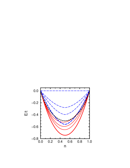
Figure 7: (Color online) Kinetic energy $E$ in the KR mean-field approximation as functions of $n$ for: AO$\pm$ (long-dashed lines) and OL state (full lines) for increasing $\gamma=0$, 0.5, 0.707, and 1 from top to bottom; the dashed line shows the kinetic energy of the FO+ state which is independent of $\gamma$.

Next we consider the variation of the total energy $E$ of ordered and disordered complex orbital states with electron filling $n$ (Fig. 7). In the spin model ($\gamma=0$) the FM phase has somewhat lower energy than the disordered OL state close to half-filling, in the range $n>2/3$.notekr Our approach reproduces in this limit the known result of the slave boson approach, which gives a FM ground state for any bipartite lattice with the density of states being an even function of energy.Moe93 When $\gamma$ is increased, $E_{\rm FO}$ does not change, whereas $E_{{\rm AO}\pm}$, initially at zero for $\gamma=0$, decreases $\propto\gamma$, and at $\gamma=1$ surpasses the FO+ state at $x=0.27$. Hence, the slave boson approach reproduces here the result of the HF approximation for these states. Tak98 However, in spite of the band narrowing $\propto q(x)$, which is appreciable at these electron densities near half-filling, considerably more (kinetic) energy is gained in the OL state. This is basically due to the fact that both hopping channels contribute, which gives rise to the large density of states over the full frequency range, and at small doping in particular [compare Fig. 1(d) with Fig. 2]. We may conclude that the presence of the additional non-pseudospin-conserving hopping channel, associated with the absence of SU(2) symmetry, implies that more kinetic energy can be gained by paying correlation energy than in the spin case, and that this favors the disordered OL state sufficiently to make its energy lower than those of the complex orbital-ordered states at any value of $n$.

Figure 8: Region of stability of the FO states at $U=\infty$ as a function of $\gamma$; the transition to the OL state from the FO$x(z)$ and complex FO+ state are shown by the full and dashed line, respectively.

Finally we compare at $U=\infty$ the energies of all states, both with complex and real orbitals, varying $n$ and $\gamma$. One finds that AO states are never stable in this limit of strong correlation, while FO states are stable only at small $\gamma$ [Fig. 8]. At $\gamma=0$ (the spin case) the FO+ and FO$x$ (FO$z$) states are necessarily degenerate, but at any $\gamma>0$ the phases with ordered real orbitals have lower energy, with FO$z$ (FO$x$) being more stable at $n<0.71$ ($n>0.71$). The range of FO order shrinks gradually with increasing $\gamma$, and above $\gamma\simeq 0.94$ the OL phase is stable in the entire range of $n$. We argue that at finite $U$ the kinetic energy will become even more dominant and thus will strongly favor disorder, except near $n\simeq 1$ where SE stabilizes real-orbital AO order.Kug82 ; Ole03 ; Fei97 ; Fei99 ; Mae00 We thus conclude that for the $e_{g}$ orbital Hubbard model ($\gamma=1$) doping triggers a crossover to the OL state at any $U$, supporting earlier conjectures that such a disordered state is realized.Nag97 ; Kil98

V.5 Brinkman-Rice transition at $n=1$

At half-filling ($n=1$) it is straightforward to apply the finite-$U$ version of the KR formalism,Kot86 and investigate the generic metal-insulator transition in the orbital disordered phase, ignoring the AO order promoted by the SE. Here one introduces as a counterpart to the bosons $e_{i}$ which control the empty configurations $|0\rangle=e_{i}^{\dagger}|{\rm vac}\rangle$, also bosons $d_{i}$ which control the double occupancies $c_{i\uparrow}^{\dagger}c_{i\downarrow}^{\dagger}|0\rangle=d_{i}^{\dagger}f_{i\uparrow}^{\dagger}f_{i\downarrow}^{\dagger}|{\rm vac}\rangle$. The mean-field approximation gives then the renormalization factor (at $n=1$),Kot86

$$\eta(d)=8d^{2}(1-2d^{2}),$$ (123)

where $d=\langle d_{i}\rangle$ is the average amplitude of a doubly occupied configuration in the ground state. The bands are then given by the dispersion for free electrons (45) renormalized by $\eta(d)$,

$$\varepsilon_{U,\pm}^{\rm OL}({\bf k})=\eta(d)\varepsilon_{U=0,\pm}({\rm k})=-\eta(d)t[A_{\bf k}\pm\gamma B_{\bf k}].$$ (124)

So the kinetic energy is $\eta(d)\bar{\epsilon}_{0}(\gamma)$, where $\bar{\epsilon}_{0}(\gamma)$ is the kinetic energy of the uncorrelated OL, obtained by integrating the two bands $\varepsilon_{U=0,\pm}({\rm k})$ (45) up to half-filling, while the Coulomb repulsion gives an energy $Ud^{2}$ per site.

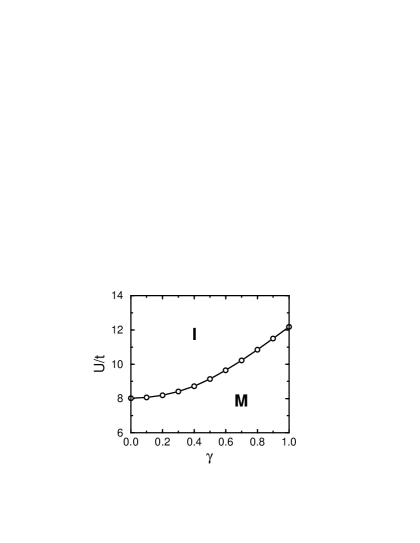
Figure 9: Metal (M) to insulator (I) transition with increasing $U$, as obtained in the disordered phase as a function of $\gamma$ at $n=1$. At $\gamma=1$ (orbital case) the transition occurs in the ground state, while at $\gamma=0$ (spin case) the result of Ref. Bri70, is reproduced.noteafi

For the spin model ($\gamma=0$) this problem was solved by Brinkman and Rice,Bri70 who showed that an ‘insulating’ state (with $d=0$) sets in above $U_{c}\simeq 8t$ (in the present units). It is well understood by now (see Ref. Faz99, ) that this mean-field theory does not give an accurate description of the metal-insulator transition (in particular it ignores all charge fluctuations in the insulating phase, where in reality $d\neq 0$).Fle04 By analogy, one expects that also in the present case $d\neq 0$ at any finite $U$, and in fact this follows from the large-$U$ expansion analyzed for the ordered phases in Secs. IV.2 and IV.3 (for a disordered phase a similar analysis could also be made). Nevertheless, the Brinkman-Rice transition from a ‘metallic’ to an ‘insulating’ state at $n=1$ illustrates nicely the competition between kinetic energy and Coulomb repulsion energy,noteafi and so it is worthwhile to consider the general case, i.e., with arbitrary $\gamma$. Then, completely analogously to the spin case, an ‘insulating’ state is found above $U_{c}(\gamma)=8|\bar{\epsilon}_{0}(\gamma)|$. Similar to what happens upon doping (i.e., at finite $x$) in the $U=\infty$ limit considered above, here upon allowing double occupancy (i.e., finite $d$) at $n=1$, the metallic phase gains additional kinetic energy $\propto\gamma$ due to non-pseudospin-conserving hopping which lowers the kinetic energy below the value due to pseudospin-conserving hopping alone (the only one present in the spin case). Therefore, the metallic phase survives up to a higher value of $U$ than at $\gamma=0$, as shown in Fig. 9.

VI Summary and Conclusions

In this paper we have made a detailed analysis of the $e_{g}$-orbital Hubbard model on a cubic lattice, exploring the consequences of the absence of SU(2) symmetry and highlighting them by making a comparison with the familiar SU(2)-symmetric spin Hubbard model. In the first part we studied the orbital-ordered phases, of which there is a great variety, precisely because of the lower symmetry, emphasizing the difference between the complex-orbital states which retain cubic symmetry, and the real-orbital states in which cubic symmetry is broken. Analytical results for the order parameter and the energy of each of these phases in the HF approximation at large $U/t$ were presented, demonstrating that the total energy can be conveniently divided into two contributions: a kinetic energy $\propto t$ given by the $U=\infty$ limit, and a SE contribution $\propto t^{2}/U$. The SE decides about the relative stability of the various phases at half-filling, while the kinetic energy contributes and finally becomes dominant upon doping. This analytical treatment allowed us: (i) to demonstrate explicitly that SE contributes in both AO and FO states, (ii) to demonstrate that the real-orbital states have their orbitals aligned with the cubic axes, as well as (iii) to elucidate the structure of the HF phase diagram for the ordered phases obtained numerically.Shi00 ; Bri01 ; Mae00 We emphasize that these properties of $e_{g}$ orbital degrees of freedom are essentially different from those of $t_{2g}$ ones, because the latter satisfy certain symmetries and are thus conserved in the hopping processes.Kha00 ; Har03

In the second part we investigated the disordered orbital-liquid state. We have demonstrated that in the strong-correlation limit ($U\gg t$) indeed orbital (FO or AO) order is not robust for $e_{g}$ orbitals, and gets replaced by a disordered (OL) phase, if one goes beyond the HF approximation and includes electron correlation effects in the disordered phase as well. This leads us to the conclusion that the HF results,Shi00 ; Mae00 ; Bri01 suggesting that either the FO+ or the AO$\pm$ state is realized in a broad range of doping, are particularly misleading for the orbital Hubbard model. Here the present findings agree qualitatively with the results of the self-consistent second order perturbation theory obtained by Kubo and Hirashima.Kub02 The situation could be somewhat different in the 2D case, however, where a tendency towards particular orbital orderings with larger amplitude of $x^{2}-y^{2}$ orbitals is favored by geometry.Mac99 ; Tha00

We considered specifically the $U=\infty$ limit, where the OL competes with fully polarized ordered phases and we have shown that it is more stable than any of either uniform FO (85) or staggered AO (86) states. However, at finite $U$ and for sufficiently low doping $x$, real-orbital $C$-AO order is stabilized by a superposition of the SE and the JT effect. Particularly in the regime of low doping the JT interactions might be stronger than the electronic interactions of double-exchange type, and the induced orbital order dictates then the type of magnetic order.Feh04 ; Dag04 This regime is particularly difficult in realistic models for manganites, as the orbital interactions induced by oxygen distortions,Fei99 and the orbital polarization around doped holesKil99 give additional important contributions and support particular types of orbital order. Furthermore, the overall stability of ordered versus disordered (OL) phases changes when a realistic Hund’s coupling is included.Mai03 It has been shown that the FM phase shrinks then to a range of doping $0.2\lesssim x\lesssim 0.5$, the $A$-type AF phase is stable near $x=0.5$, while the $C$-AF phase takes over at higher hole doping.

Summarizing, the absence of SU(2) symmetry in the $e_{g}$-orbital Hubbard model has severe consequences for the properties of the model itself and for the stability of orbital-ordered states. The Nagaoka theorem does not apply to the model of correlated $e_{g}$ electrons at $U=\infty$, ordered states are harder to realize than in the spin case, and the Brinkman-Rice transition occurs at a higher value of $U$. The qualitatively different properties of the ordered phases show up most clearly in the inverted stability (with respect to the spin case) of the ordered phases with complex orbitals, with ferro (staggered) orbital order favored at small (large) doping. Most importantly, the exciting suggestion that such complex-orbital ordered states could be stable at finite dopingBri01 ; Shi00 ; Mae00 has been disproved, because of the inherent tendency of $e_{g}$ systems towards orbital disorder due to the enhancement of the kinetic energy when SU(2) symmetry is absent. All these features show that several properties of spin systems which are usually taken for granted, such as: (i) the very fact that a ferromagnetic state is an eigenstate of either an itinerant or the Heisenberg Hamiltonian, and (ii) the absence of superexchange in ferromagnetic states — are in fact the consequences of the SU(2) symmetry of the respective spin models.

*

Appendix A slave boson representation for real orbitals

The real-orbital version of the transformation of the electron operators to slave boson and pseudofermion operators may be derived by making repeated use of the relation between the real and complex orbitals, as given by Eqs. (4). Thus with the real-orbital electron operators given by

$$c_{iz}^{\dagger} = \textstyle{\frac{1}{\sqrt{2}}}\Big{(}c_{i+}^{\dagger}+c_{i-}^{\dagger}\Big{)},$$

$$c_{ix}^{\dagger} = \textstyle{\frac{i}{\sqrt{2}}}\Big{(}c_{i+}^{\dagger}-c_{i-}^{\dagger}\Big{)},$$ (125)

we similarly define the real-orbital pseudofermion operators by

$$f_{iz}^{\dagger} = \textstyle{\frac{1}{\sqrt{2}}}\Big{(}f_{i+}^{\dagger}+f_{i-}^{\dagger}\Big{)},$$

$$f_{ix}^{\dagger} = \textstyle{\frac{i}{\sqrt{2}}}\Big{(}f_{i+}^{\dagger}-f_{i-}^{\dagger}\Big{)},$$ (126)

while for the slave boson operators we set

$$b_{iz}^{\dagger} = \textstyle{\frac{1}{\sqrt{2}}}\Big{(}b_{i+}^{\dagger}+b_{i-}^{\dagger}\Big{)},$$

$$b_{ix}^{\dagger} = \textstyle{\frac{-i}{\sqrt{2}}}\Big{(}b_{i+}^{\dagger}-b_{i-}^{\dagger}\Big{)}.$$ (127)

Then the fermions (electrons) transform under U(1) rotations as

$$\hat{U}_{i}(\theta)c_{iz}^{\dagger}\hat{U}_{i}^{\dagger}(\theta) = \cos(\theta/2)\>c_{iz}^{\dagger}-\sin(\theta/2)\>c_{ix}^{\dagger},$$

$$\hat{U}_{i}(\theta)c_{ix}^{\dagger}\hat{U}_{i}^{\dagger}(\theta) = \sin(\theta/2)\>c_{iz}^{\dagger}+\cos(\theta/2)\>c_{ix}^{\dagger},$$ (128)

and similarly for the pseudofermions, while the slave bosons transform as

$$\hat{U}_{i}(\theta)b_{iz}^{\dagger}\hat{U}_{i}^{\dagger}(\theta)= \cos\theta\>b_{iz}^{\dagger}+\sin\theta\>b_{ix}^{\dagger},$$

$$\hat{U}_{i}(\theta)b_{ix}^{\dagger}\hat{U}_{i}^{\dagger}(\theta)= - \sin\theta\>b_{iz}^{\dagger}+\cos\theta\>b_{ix}^{\dagger}.$$ (129)

The different sign choice in Eq. (127) as compared to Eqs. (125) and (126) makes the slave bosons rotate in the opposite direction as the (pseudo)fermions. This compensates for the doubled rotation angle in the sense that the transformations are identical for slave bosons and (pseudo)fermions when $\theta$ is a cubic angle, and so the pairs $\{c_{iz}^{\dagger},c_{ix}^{\dagger}\}$, $\{f_{iz}^{\dagger},f_{ix}^{\dagger}\}$, and $\{b_{iz}^{\dagger},b_{ix}^{\dagger}\}$ all transform as the $\theta$ and $\epsilon$ component of a cubic $E$ doublet.

Substituting the complex-orbital slave boson representation (97) into Eq. (125) and applying the inverse transformations to (126) and (127), one obtains the slave boson representation for the real-orbital fermionic operators $\{c_{iz}^{\dagger},c_{ix}^{\dagger}\}$ analogous to Eq. (97). The result is

$$c_{iz}^{\dagger} = +\textstyle{\frac{1}{\sqrt{2}}}\Big{(}b_{iz}^{\dagger}f_{iz}^{\dagger}-b_{ix}^{\dagger}f_{ix}^{\dagger}\Big{)}e_{i},$$

$$c_{ix}^{\dagger} = -\textstyle{\frac{1}{\sqrt{2}}}\Big{(}b_{ix}^{\dagger}f_{iz}^{\dagger}+b_{iz}^{\dagger}f_{ix}^{\dagger}\Big{)}e_{i},$$ (130)

corresponding to a representation of the local states by

$$|i0\rangle = e_{i}^{\dagger}|{\rm vac}\rangle,$$

$$|iz\rangle=c_{iz}^{\dagger}|i0\rangle = +\textstyle{\frac{1}{\sqrt{2}}}\Big{(}b_{iz}^{\dagger}f_{iz}^{\dagger}-b_{ix}^{\dagger}f_{ix}^{\dagger}\Big{)}|{\rm vac}\rangle,$$

$$|ix\rangle=c_{ix}^{\dagger}|i0\rangle = -\textstyle{\frac{1}{\sqrt{2}}}\Big{(}b_{ix}^{\dagger}f_{iz}^{\dagger}+b_{iz}^{\dagger}f_{ix}^{\dagger}\Big{)}|{\rm vac}\rangle.$$ (131)

One recognizes that Eqs. (130) are indeed the proper expressions for the $E$ doublet resulting from the product representation $E\otimes E\otimes A_{1}$. Grif The expressions (130) are actually even U(1)-invariant, i.e., after a rotation in orbital space by an arbitrary angle $\theta$, they also hold between the fermion operators $\{c_{iz}^{\prime\dagger},c_{ix}^{\prime\dagger}\}=\{\hat{U}_{i}(\theta)c_{iz}^{\dagger}\hat{U}_{i}^{\dagger}(\theta),\hat{U}_{i}(\theta)c_{ix}^{\dagger}\hat{U}_{i}^{\dagger}(\theta)\}$, transformed according to Eq. (128), and the slave boson and pseudofermion operators $\{b_{iz}^{\prime\dagger},b_{ix}^{\prime\dagger}\}$ and $\{f_{iz}^{\prime\dagger},f_{ix}^{\prime\dagger}\}$, transformed according to Eqs. (129) and (128), respectively. Consequently, since the hopping Hamiltonian (3) is invariant under a transformation (128) of the fermion (electron) operators when $\theta$ is one of the cubic angles $0,\pm 4\pi/3$ and is accompanied by the corresponding permutation of the cubic axes, this cubic invariance is retained when the Hamiltonian is expressed in terms of the slave boson and pseudofermion operators by means of Eq. (130).

The constraints given by Eqs. (100) are now replaced by

$$b_{iz}^{\dagger}b_{iz}+b_{ix}^{\dagger}b_{ix} + e_{i}^{\dagger}e_{i}=1,$$

$$b_{iz}^{\dagger}b_{iz}+b_{ix}^{\dagger}b_{ix} = f_{iz}^{\dagger}f_{iz}+f_{ix}^{\dagger}f_{ix},$$

$$b_{iz}^{\dagger}b_{ix}-b_{ix}^{\dagger}b_{iz} = f_{iz}^{\dagger}f_{ix}-f_{ix}^{\dagger}f_{iz}.$$ (132)

Again the first constraint excludes double-occupancy, as required in the limit $U=\infty$, while the last constraint is readily verified to eliminate the unphysical singly-occupied states,

$$|iA_{1}\rangle = \textstyle{\frac{1}{\sqrt{2}}}\Big{(}b_{iz}^{\dagger}f_{iz}^{\dagger}+b_{ix}^{\dagger}f_{ix}^{\dagger}\Big{)}|{\rm vac}\rangle,$$

$$|iA_{2}\rangle = \textstyle{\frac{1}{\sqrt{2}}}\Big{(}b_{ix}^{\dagger}f_{iz}^{\dagger}-b_{iz}^{\dagger}f_{ix}^{\dagger}\Big{)}|{\rm vac}\rangle.$$ (133)

When the constraints are obeyed rigorously and the unphysical states strictly projected out, operators connecting the physical and unphysical subspaces necessarily vanish identically. Specifically one finds

$$b_{iz}^{\dagger}b_{iz}-b_{ix}^{\dagger}b_{ix}=f_{iz}^{\dagger}f_{iz}-f_{ix}^{\dagger}f_{ix} = 0,$$

$$b_{iz}^{\dagger}b_{ix}+b_{ix}^{\dagger}b_{iz}=f_{iz}^{\dagger}f_{ix}+f_{ix}^{\dagger}f_{iz} = 0.$$ (134)

It is obvious from the above that the earlier attempt made in Ref. Ole00, to construct a real-orbital slave boson representation by means of $c_{iz}^{\dagger}=b_{iz}^{\dagger}f_{iz}^{\dagger}e_{i}$ and $c_{ix}^{\dagger}=b_{ix}^{\dagger}f_{ix}^{\dagger}e_{i}$, followed by renormalization of the slave boson factors by

$$z_{iz}^{\dagger} = \frac{b_{iz}^{\dagger}e_{i}}{\sqrt{(1-e_{i}^{\dagger}e_{i}-b_{ix}^{\dagger}b_{ix})(1-b_{iz}^{\dagger}b_{iz})}},$$

$$z_{ix}^{\dagger} = \frac{b_{ix}^{\dagger}e_{i}}{\sqrt{(1-e_{i}^{\dagger}e_{i}-b_{iz}^{\dagger}b_{iz})(1-b_{ix}^{\dagger}b_{ix})}},$$ (135)

was misguided because it does not conserve the cubic symmetry, and is thus bound to lead to spurious results. However, also the present real-orbital representation, though invariant in itself, leaves us with the problem to construct a proper cubic-invariant renormalization. This is not straighforward because the hopping Hamiltonian, when expressed completely in terms of slave boson and pseudofermion operators referring to ‘$z$’ and ‘$x$’, takes a different appearance for each cubic axis, like in Eq. (3). Moreover, the apparently plausible renormalization by means of Eqs. (135) is not allowed even in combination with the representation (130), because $z_{iz}^{\dagger}$ and $z_{ix}^{\dagger}$ as defined by Eqs. (135) do not constitute a cubic $E$ doublet as their denominators are not cubic invariants. Having them replace $b_{iz}^{\dagger}e_{i}$ and $b_{ix}^{\dagger}e_{i}$ in Eqs. (130) would spoil also the cubic $E$ doublet nature of the thus renormalized $c_{iz}^{\dagger}$ and $c_{ix}^{\dagger}$, and so destroy the cubic symmetry of the Hamiltonian. Equally seriously, it would also cause the Hamiltonian to commute no longer with the constraints.

A renormalization not suffering from the above problems and still in the spirit of the Kotliar-Ruckenstein AnsatzKot86 is given by

$$z_{iz}^{\dagger} = \frac{b_{iz}^{\dagger}e_{i}}{\sqrt{(1-e_{i}^{\dagger}e_{i}-\textstyle{\frac{1}{2}}n_{i}^{(b)})(1-\textstyle{\frac{1}{2}}n_{i}^{(b)})}},$$

$$z_{ix}^{\dagger} = \frac{b_{ix}^{\dagger}e_{i}}{\sqrt{(1-e_{i}^{\dagger}e_{i}-\textstyle{\frac{1}{2}}n_{i}^{(b)})(1-\textstyle{\frac{1}{2}}n_{i}^{(b)})}},$$ (136)

where $n_{i}^{(b)}=b_{iz}^{\dagger}b_{iz}+b_{ix}^{\dagger}b_{ix}$. The mean-field approximation is now made, as in Sec. V.1, by replacing only the amplitudes but not the phases by c-numbers. So, for the offdiagonal two-boson products we set, similarly to what was done in Eqs. (108),

$$\langle b_{iz}^{\dagger}e_{i}\rangle \equiv \langle e_{i}^{\dagger}b_{iz}\rangle\equiv\bar{b}_{i}\bar{e}_{i}\>\cos(\alpha_{i}-\hat{\vartheta}_{i}),$$

$$\langle b_{ix}^{\dagger}e_{i}\rangle \equiv \langle e_{i}^{\dagger}b_{ix}\rangle\equiv\bar{b}_{i}\bar{e}_{i}\>\sin(\alpha_{i}-\hat{\vartheta}_{i}).$$ (137)

where $\bar{b}_{i}$ and $\bar{e}_{i}$ are again real quantities. For the diagonal two-boson products we set

$$\langle b_{iz}^{\dagger}b_{iz}\rangle \equiv \langle b_{ix}^{\dagger}b_{ix}\rangle\equiv\textstyle{\frac{1}{2}}\bar{b}_{i}^{2}$$

$$\langle e_{i}^{\dagger}e_{i}\rangle \equiv \bar{e}_{i}^{2}.$$ (138)

Actually, the real-orbital boson occupation numbers $n_{iz}^{(b)}=b_{iz}^{\dagger}b_{iz}$ and $n_{ix}^{(b)}=b_{ix}^{\dagger}b_{ix}$ are not invariants with respect to U(1) rotations, and so one would prefer to set, in accordance with Eqs. (137), the corresponding diagonal averages equal to

$$\langle b_{iz}^{\dagger}b_{iz}\rangle \equiv \bar{b}_{i}^{2}\>\cos^{2}(\alpha_{i}-\hat{\vartheta}_{i}),$$

$$\langle b_{ix}^{\dagger}b_{ix}\rangle \equiv \bar{b}_{i}^{2}\>\sin^{2}(\alpha_{i}-\hat{\vartheta}_{i}),$$ (139)

in order to make them transform in the same way as the occupation numbers, by setting also

$$\langle b_{iz}^{\dagger}b_{ix}\rangle\equiv\langle b_{ix}^{\dagger}b_{iz}\rangle\equiv\textstyle{\frac{1}{2}}\bar{b}_{i}^{2}\>\sin(2\alpha_{i}-2\hat{\vartheta}_{i}).$$ (140)

However, the expressions (139) and (140) do not satisfy Eqs. (134), and so it appears to be impossible to assign a nontrivial dependence on the phase operator $\hat{\vartheta}_{i}$ to $\langle b_{iz}^{\dagger}b_{iz}\rangle$ and $\langle b_{ix}^{\dagger}b_{ix}\rangle$ and yet simultaneously respect (134).

The issue is immaterial for carrying out the KR procedure, since in a state with uniform density, i.e. with $\bar{e}_{i}^{2}=x$ for all $i$, it follows from the constraints (132) that both for (138) and for (139) the amplitude satisfies $\bar{b}_{i}^{2}=1-x$, so that

$$\langle z_{iz}^{\dagger}\rangle \equiv \langle z_{iz}\rangle\equiv\sqrt{2q(x)}\;\cos(\alpha_{i}-\hat{\vartheta}_{i}),$$

$$\langle z_{ix}^{\dagger}\rangle \equiv \langle z_{ix}\rangle\equiv\sqrt{2q(x)}\;\sin(\alpha_{i}-\hat{\vartheta}_{i}).$$ (141)

Inserting this into Eqs. (130) and defining new pseudofermions by

$$\hat{\hat{f}}_{iz}^{\dagger} = \hskip 8.5359pt\cos\alpha_{i}\>\hat{f}_{iz}^{\dagger}+\sin\alpha_{i}\>\hat{f}_{ix}^{\dagger},$$

$$= \hskip 8.5359pt\cos(\hat{\vartheta}_{i}-\alpha_{i})\>f_{iz}^{\dagger}+\sin(\hat{\vartheta}_{i}-\alpha_{i})\>f_{ix}^{\dagger},$$

$$\hat{\hat{f}}_{ix}^{\dagger} = -\sin\alpha_{i}\>\hat{f}_{iz}^{\dagger}+\cos\alpha_{i}\>\hat{f}_{ix}^{\dagger},$$

$$= \hskip 8.5359pt\sin(\hat{\vartheta}_{i}-\alpha_{i})\>f_{iz}^{\dagger}-\cos(\hat{\vartheta}_{i}-\alpha_{i})\>f_{ix}^{\dagger},$$

where $\{\hat{f}_{iz}^{\dagger},\hat{f}_{ix}^{\dagger}\}$ are related to $\{\hat{f}_{i+}^{\dagger},\hat{f}_{i-}^{\dagger}\}$ [see Eq. (113)] by Eqs. (126), one finds that the mean-field approximation effectively leads to the replacements

$$c_{iz}^{\dagger}\equiv\sqrt{q(x)}\hat{\hat{f}}_{iz}^{\dagger},\hskip 19.91684ptc_{ix}^{\dagger}\equiv\sqrt{q(x)}\hat{\hat{f}}_{ix}^{\dagger}.$$ (143)

The kinetic part of the Hamiltonian is thus simply renormalized by the Gutzwiller factor $q(x)$, exactly the same result as obtained in the complex-orbital approach. As the Hamiltonian is therefore again cubic, it follows that the resulting real-orbital OL is isotropic (i.e. $\alpha_{i}=\pi/4$ at all sites, and $\langle b_{iz}^{\dagger}b_{iz}\rangle=\langle b_{ix}^{\dagger}b_{ix}\rangle=(1-x)/2$), and identical to the OL obtained in the complex-orbital approach.

References

- (1) Y. Tokura and N. Nagaosa, Science 288, 462 (2000); S. Maekawa, T. Tohyama, S. E. Barnes, S. Ishihara, W. Koshibae, and G. Khaliullin, Physics of Transition Metal Oxides (Springer Verlag, Berlin, 2004).
- (2) K. I. Kugel and D. I. Khomskii, Usp. Fiz. Nauk 136, 621 (1982) [Sov. Phys. Usp. 25, 231 (1982)]; A. M. Oleś, L. F. Feiner, and J. Zaanen, Phys. Rev. B61, 6257 (2000).
- (3) A. M. Oleś, Phys. Stat. Sol. (b) 236, 281 (2003).
- (4) L. F. Feiner, A. M. Oleś, and J. Zaanen, Phys. Rev. Lett. 78, 2799 (1997).
- (5) G. Khaliullin and S. Maekawa, Phys. Rev. Lett. 85, 3950 (2000); G. Khaliullin, Phys. Rev. B64, 212405 (2001); G. Khaliullin, P. Horsch, and A. M. Oleś, Phys. Rev. Lett. 86, 3879 (2001).
- (6) L. F. Feiner and A. M. Oleś, Phys. Rev. B59, 3295 (1999).
- (7) M. Imada, A. Fujimori, and Y. Tokura, Rev. Mod. Phys. 70, 1039 (1998); E. Dagotto, T. Hotta, and A. Moreo, Phys. Rep. 344, 1 (2001); E. Dagotto, Nanoscale Phase Separation and Colossal Magnetoresistance (Springer-Verlag, Heidelberg, 2003).
- (8) C. Zener, Phys. Rev. 82, 403 (1951).
- (9) A. Weiße, J. Loos, and H. Fehske, Phys. Rev. B64, 054406 (2001); 68, 024402 (2003).
- (10) S. Maezono, S. Ishihara, and N. Nagaosa, Phys. Rev. B57, R13993 (1998); 58, 11583 (1998).
- (11) S. E. Barnes, J. Phys. F 6, 115 (1976); 6, 1376 (1976).
- (12) A. M. Oleś and L. F. Feiner, Phys. Rev. B65, 052414 (2002).
- (13) Y. Endoh and K. Hirota, J. Phys. Soc. Jpn. 66, 2264 (1997).
- (14) G. Kotliar and A. E. Ruckenstein, Phys. Rev. Lett. 57, 1362 (1986).
- (15) A. Takahashi and H. Shiba, Eur. Phys. J. B 5, 413 (1998).
- (16) J. van den Brink and D. I. Khomskii, Phys. Rev. Lett. 82, 1016 (1999).
- (17) The seemingly illogical sign choice is in accordance with the Jahn-Teller literature and makes sure that [see Eq. (5)] and not is the electronic part of the conserved local pseudo angular momentum in the Jahn-Teller problem with local Jahn-Teller interaction , where and are the coordinates of the degenerate vibrational modes at site , and and are the conjugate momenta; compare: H. C. Longuet-Higgins, U. Öpik, M. H. L. Pryce, and R. A. Sack, Proc. Roy. Soc. A 244, 1 (1958); R. Englman, The Jahn-Teller Effect in Molecules and Crystals (Wiley, London, 1972), section 3.2.1.
- (18) J. Klauder, Phys. Rev. D19, 2349 (1979).
- (19) Note that is the azimuthal, not the polar angle. Here we thus follow the common practice in the orbital and Jahn-Teller literature. However, we do not follow the Jahn-Teller convention of replacing by , which would yield conveniently but would upset the standard form of the pseudospin vector Eq. (7).
- (20) J. van den Brink and D. I. Khomskii, Phys. Rev. B63, 140416 (2001).
- (21) The complete argument is actually more subtle, because the EQM has an offdiagonal matrix element between and . — The , , components of in the complex-orbital basis correspond to the pseudospin components represented in the conventional real basis by the Pauli matrices , , and , respectively, and so only and appear in the JT coupling, while is the electronic part of the conserved pseudo angular momentum; compare Ref. noteJTconv, .
- (22) P. Fazekas, Lecture Notes on Electron Correlation and Magnetism (World Scientific, Singapore, 1999).
- (23) A. Takahashi and H. Shiba, J. Phys. Soc. Jpn. 69, 3328 (2000).
- (24) S. Maezono and N. Nagaosa, Phys. Rev. B62, 11576 (2000).
- (25) S.-Q. Shen, R. Y. Gu, Q.-H. Wang, Z. D. Wang, and X. C. Xie, Phys. Rev. B62, 5829 (2000).
- (26) Note that the mixed constraint (14) behaves differently from the similar constraint satisfied by slave bosons alone in Eqs. (100), where in mean-field approximation the boson amplitudes depend on the actual electron density [see Eqs. (110)]. Here the amplitude of the fermions controls the boson amplitudes at finite doping, and the constraint remains observed when Eqs. (15) are used.
- (27) The dispersion of the bandsTak98 associated with the components due to the planes is also frequently described using which gives equivalent expressions to those given in Sec. III.
- (28) F. Mack and P. Horsch, Phys. Rev. Lett. 82, 3160 (1999).
- (29) S. Maezono and N. Nagaosa, Phys. Rev. B61, 1825 (2000).
- (30) A. Koizumi, S. Miyaki, Y. Kakutani, H. Koizumi, N. Hiraoka, K. Makoshi, N. Sakai, K. Hirota, and Y. Murakami, Phys. Rev. Lett. 86, 5589 (2001).
- (31) T. G. Perring, G. Aeppli, S. M. Hayden, S. A. Carter, J. P. Remeika, and S.-W. Cheong, Phys. Rev. Lett. 77, 711 (1996).
- (32) J. A. Fernandez-Baca, P. Dai, H. Hwang, C. Kloc, and S.-W. Cheong, Phys. Rev. Lett. 80, 4012 (1998).
- (33) It further follows from Eq. (25) that for a general (i.e., not “antiferro”) AO state the dispersion reduces in the spin case () to [as shown explicitly for the real case by Eq. (29)], which is the well-known single-band double-exchange result with being the angle between pseudospins and [cf. P.-G. de Gennes, Phys. Rev. 118, 141 (1960)].
- (34) The orbital order in the low-temperature phase of the undoped 3D manganite LaMnO3 is in between -AO and -AO [see J. Rodríguez-Carvajal, M. Hennion, F. Moussa, A. H. Moudden, L. Pinsard, and A. Revcolevschi, Phys. Rev. B57, R3189 (1998)].
- (35) A. Weiße and H. Fehske, New J. Phys. 6, 158 (2004).
- (36) Formally the situation at zero doping is anomalous. The equation for remains valid at and so , i.e. , but becomes undetermined, implying that the stable real AO solution is ‘antiferro’ () but that the common axis of the pseudospin vectors has an arbitrary direction in the ‘equatorial’ plane. This is due to the fact that the angle between the pseudospin vectors is determined by the SE energy (see Sections IV.2 and IV.3), while the average direction is selected by the kinetic energy, which is zero, though, at and thus ineffective.
- (37) In order to obtain the equations which include this deviation one should replace by in Eqs. (90) and (93) and also in Eq. (93) replace by , and then determine by minimizing the energy. At small this yields , as stated in Section IV.
- (38) Q. Yuan, T. Yamamoto, and P. Thalmeier, Phys. Rev. B62, 12696 (2000).
- (39) W. von der Linden and D. M. Edwards, J. Phys.: Conden. Matter 3, 4917 (1991).
- (40) While was expressed in Eq. (94) in terms of the original fermions, here it has to be expressed in terms of the slave bosons and pseudofermions: , where and .
- (41) R. Frésard and P. Wölfle, Int. J. Mod. Phys. B 6, 685 (1992); 6, 3087 (1992).
- (42) Therefore the present slave boson representation does not simplify the treatment of the Jahn-Teller effect; compare Ref. noteJTconv, .
- (43) This prescription is handled more naturally in a path integral formulation with the boson field represented in the radial gauge, as in Ref. Fre92, , and the modulus fields replaced by their mean-field value. The redefinition of the pseudofermion operators, Eq. (113), is equivalent to the local gauge transformation that eliminates the phase fields.
- (44) M. C. Gutzwiller, Phys. Rev. 137, A1726 (1965); D. Vollhardt, Rev. Mod. Phys. 56, 99 (1984).
- (45) Equivalent results are therefore obtained for the orbital ordered states by a single slave fermion approach.
- (46) J. Spałek and W. Wójcik, Phys. Rev. B37, 1532 (1988); J. Spałek, ibid. 40, 5180 (1989).
- (47) The nonvariational slave fermion approximation gives a different band renormalization [S. Ishihara, M. Yamanaka, and N. Nagaosa, Phys. Rev. B56, 686 (1997)], and underestimates the stability of the OL phase.
- (48) Y. Nagaoka, Phys. Rev. 147, 392 (1966).
- (49) B. Moeller, K. Doll, and R. Frésard, J. Phys.: Condens. Matter 5, 4847 (1993).
- (50) We note that the value of the critical doping is very close indeed to found for a single spin-flip in the Gutzwiller wave function for a cubic lattice [B. S. Shastry, H. R. Krishnamurthy, and P. W. Anderson, Phys. Rev. B41, 2375 (1990)].
- (51) R. Kilian and G. Khaliullin, Phys. Rev. B58, R11841 (1998).
- (52) W. F. Brinkman and T. M. Rice, Phys. Rev. B2, 4302 (1970).
- (53) M. Fleck, M. G. Zacher, A. I. Lichtenstein, W. Hanke, and A. M. Oleś, Eur. Phys. J. B 37, 439 (2004).
- (54) Note, however, that due to the Fermi surface instability the AF phase, with a gap depending on , has a lower energy in the entire range of (see, e.g., Ref. Fle04, ).
- (55) A. B. Harris, T. Yildirim, A. Aharony, O. Entin-Wohlman, and I. Y. Korenblit, Phys. Rev. Lett. 91, 087206 (2003); Phys. Rev. B69, 035107 (2004).
- (56) K. Kubo and D. S. Hirashima, J. Phys. Soc. Jpn. 71, 183 (2002).
- (57) M. Daghofer, A. M. Oleś, and W. von der Linden, Phys. Rev. B70, 184430 (2004); Phys. Stat. Sol. (b) 242, 311 (2005).
- (58) R. Kilian and G. Khaliullin, Phys. Rev. B58, 13458 (1999).
- (59) T. Maitra and A. Taraphder, Phys. Rev. B68, 174416 (2003).
- (60) J. S. Griffith, The Theory of Transition Metal Ions (Cambridge University Press, Cambridge, 1971), p. 396.
- (61) A. M. Oleś and L. F. Feiner, Acta Phys. Pol. A 97, 193 (2000).