Classical potential describes martensitic phase transformations between the $\alpha$, $\beta$ and $\omega$ titanium phases.

Abstract

A description of the martensitic transformations between the $\alpha$, $\beta$ and $\omega$ phases of titanium that includes nucleation and growth requires an accurate classical potential. Optimization of the parameters of a modified embedded atom potential to a database of density-functional calculations yields an accurate and transferable potential as verified by comparison to experimental and density functional data for phonons, surface and stacking fault energies and energy barriers for homogeneous martensitic transformations. Molecular dynamics simulations map out the pressure-temperature phase diagram of titanium. For this potential the martensitic phase transformation between $\alpha$ and $\beta$ appears at ambient pressure and 1200 K, between $\alpha$ and $\omega$ at ambient conditions, between $\beta$ and $\omega$ at 1200 K and pressures above 8 GPa, and the triple point occurs at 8GPa and 1200 K. Molecular dynamics explorations of the dynamics of the martensitic $\alpha-\omega$ transformation show a fast-moving interface with a low interfacial energy of 30 meV/Ų. The potential is applicable to the study of defects and phase transformations of Ti.

I Introduction

Martensitic phase transitions control systems ranging from shape memory alloysOtsuka and Wayman (1998) to steelsOlson and Owen (1992) to planetary cores.Vočadlo et al. (2003) They are diffusionless structural transformations proceeding near the speed of sound.Olson and Owen (1992) Martensitic transformations frequently appear in alloy design as a way to improve materials properties, but their occurrence can also limit materials performance.

Titanium’s great technological importanceLütjering and Williams (2003) makes it an ideal example for the development of physics-based predictive methods for materials problems. Titanium displays several phases as a function of pressure and temperature. At ambient conditions titanium stabilizes in the hexagonal close-packed (hcp) $\alpha$ phase. At ambient pressure and temperatures above 1155 K the $\alpha$ phase transforms to the high-temperature body-centered cubic (bcc) $\beta$ phase. Under pressure the $\alpha$ phase transforms into the hexagonal $\omega$ phase.Jamieson (1963) The high-pressure $\omega$ phase consist of a three atom hexagonal structure equivalent to AlB₂ with Ti occupying sites of alternating triangular and honeycomb layers. The crystal structure of Ti at 0 K has not been determined experimentally. Extrapolation of the $\alpha$-$\omega$ phase boundarySikka et al. (1982) in Ti indicates $\omega$ as the ground state phase. Free energy calculations of $\alpha$ and $\omega$ within the quasiharmonic approximation using a TB model show phonon entropy stabilizing the $\alpha$ phase at ambient temperature.Rudin et al. (2004) Ti displays martensitic transformations between its $\alpha$ (hcp), $\beta$ (bcc) and $\omega$ (hexagonal) phases. Two-phase $\alpha$/$\beta$ alloys make up many industrial titanium alloys such as Ti-6Al-4V because the presence of $\beta$ phase in the $\alpha$ matrix improves strength and creep resistance.Lütjering and Williams (2003) Titanium transforms from $\alpha$ to brittle $\omega$ under pressure creating serious technological problems for $\beta$ stabilized titanium alloys. Impurities greatly affect the $\alpha$ to $\omega$ transformation; for example, as little as 1 at.% oxygen in commercial Ti alloys suppresses it.Vohra et al. (1977); Gray et al. (1993); Hennig et al. (2005)

To understand these transformations in Ti and its alloys we begin with the study of the phase transformations in pure titanium. Our approach to a theoretical understanding of these transformation involves three steps: (1) find the homogeneous atomistic pathway of the martensitic transformation in pure titanium, (2) use this pathway to estimate the effect of impurities, and (3) determine the heterogeneous nucleation and dynamics of the martensitic phase transformation.

The homogeneous transformation pathway for all three martensitic transformations in Ti is known. Burgers described the $\alpha$ to $\beta$ transformation in Zr;Burgers (1934) the same mechanism occurs in Ti. The $\beta$ to $\omega$ transformation occurs via plane collapse along the $[111]$ direction corresponding to the longitudinal $\frac{2}{3}[111]$ phonon.Hatt and Roberts (1960); de Fontaine (1970); Persson et al. (2000) More recently Trinkle et al. determined the homogeneous pathway of the $\alpha$ to $\omega$ transformation.Trinkle et al. (2003, 2005) A systematic approach generated all possible pathways that were then successively pruned by energy estimates using elastic theory, tight-binding (TB) methods and density-functional theory (DFT).

The speed of the diffusionless martensitic transformation traps dilute impurities, providing candidate pathways for alloyed materials. Hennig et al. determined the effect of interstitial and substitutional impurities on the $\alpha$ to $\omega$ transformation.Hennig et al. (2005) DFT nudged-elastic band refinements yield the change in both the relative stability of and the energy barrier between the phases due to impurities. The resulting microscopic picture explains the suppression of the $\alpha$ to $\omega$ transformation in commercial Ti alloys.

The final step involves studying the full atomistic dynamics of the nucleation and growth of the martensitic phase; this requires molecular dynamics simulations of large systems. For the required system sizes an accurate quantum mechanical treatment by DFT or TB methods becomes too computationally demanding. Such simulations call for a classical potential to allow the treatment of appropriate length and time scales for nucleation and growth of martensites.

In this paper we develop a classical potential of the modified embedded atom methodLenosky et al. (2000) (MEAM) type for Ti. The potential accurately describes the stability of the $\alpha$, $\beta$ and $\omega$ phases and is applied to study the dynamics of the martensitic $\alpha$ to $\omega$ transformation and the interfacial energy between the $\alpha$ and $\omega$ phase. Section II describes the calculations for the DFT database, the functional form of the MEAM potential and the optimization of the potential parameters to the DFT database. The accuracy of the potential is tested by comparing phonon spectra, surface and stacking fault energies as well as energy barriers for homogeneous martensitic transformations to DFT, TB and experimental results. In Section III we apply the potential to study the phase diagram of Ti and the martensitic phase transformations between the phases. We estimate the interfacial energy between $\alpha$ and $\omega$ and show that the classical MEAM potential accurately describes the stability range of the three Ti phases and the phase transformations between them.

II Optimization of the classical potential to density functional database

To describe the interactions between the Ti atoms and to enable large-scale molecular dynamics simulations we develop a classical potential. The modified embedded atom method provides the form of the potentialLenosky et al. (2000) with potential parameters optimized to a database of DFT calculations. A second DFT database provides testing data for the potential. The optimization of the model proceeds iteratively. Systematically adding DFT results to the fitting and testing databases improves the accuracy and extends the applicability of the model. This enables the development of a potential that accurately reproduces the properties of all three Ti phases relevant for the description of the martensitic phase transitions. Available experimental data confirms the accuracy of the resulting Ti MEAM potential.

II.1 Density functional calculations

The DFT calculations are performed with Vasp,Kresse and Hafner (1993); Kresse and Furthmüller (1996) a density functional code using a plane-wave basis and ultrasoft Vanderbilt type pseudopotentials.Vanderbilt (1990); Kresse and Hafner (1994) The generalized gradient approximation (GGA) of Perdew and Wang is used.Perdew (1991) A plane-wave kinetic energy cutoff of 400 eV ensures energy convergence to 0.3 meV/atom. The $k$-point meshes for the different structures are chosen to guarantee an energy accuracy of 1 meV/atom. We treat the Ti $3p$ states as valence states in addition to the usual $4s$ and $3d$ states to provide an accurate treatment of the interaction at close interatomic distances.

The DFT database for the fitting of the potential parameters consists of energies, defects, forces and elastic constants for a variety of Ti phases as well as energies of configurations along the TAO-1 transformation pathway from $\alpha$ to $\omega$.Trinkle et al. (2003, 2005) Relaxations determine the ground state energies and lattice parameters of the $\alpha$, $\beta$, $\omega$, fcc, A15 and simple hexagonal phases. The volume dependence of the energy for $\alpha$, $\beta$, $\omega$, fcc and A15 and the elastic constants of the $\alpha$, $\beta$ and $\omega$ phases at their equilibrium volumes are calculated. Snapshots of short DFT molecular dynamics simulations for $\alpha$, $\beta$ and $\omega$ at 800 K at their respective ground state volumes with and without a vacancy defect provide force-matching data.Ercolessi and Adams (1994) Defect structures and formation energies are determined by relaxations for single vacancies and single interstitial atoms in a 96-atom ($4\times 4\times 3$) supercell for $\alpha$ and a 108-atom ($3\times 3\times 4$) supercell for $\omega$ with a $2\times 2\times 2$ $k$-point sampling grid. This results in a 1 at.% defect concentration. The atom positions are relaxed until the atomic-level forces are smaller than 20 meV/Å.

The DFT database for the test of the accuracy of the potential consists of additional interstitial defects in $\alpha$ and $\omega$, phonon spectra for $\alpha$, $\beta$ and $\omega$, surface energies for $\alpha$ and $\omega$, and the I₂ stacking fault in $\alpha$. The phonon calculation employ the direct force method and supercells of 150 atoms ($5\times 5\times 3$) for $\alpha$, 125 atoms ($5\times 5\times 5$) for $\beta$, and 135 atoms ($3\times 3\times 5$) for $\omega$. The surfaces are constructed by separating the crystal along a high-index plane. The surface energies result from relaxing a periodic stacking of an 18 Å to 20 Å thick slab of rectangular hcp cells with a 10 Å vacuum region and a perfect bulk cell with the same cell vectors. A $k$-point mesh equivalent to $13\times 13\times 1$ is used for both the bulk and the slab calculation. Relaxations of a $1\times 1\times 5$ supercell of $\alpha$ with and without a single I₂ stacking fault determine the stacking fault energy.

Comparison to available experimental data for phonon spectra, surface energies, the stacking fault in $\alpha$, and the $p$-$T$ phase diagram of Ti further confirm the accuracy of the potential as do approximate energy barriers for homogeneous martensitic transformations in TB.

II.2 Modified embedded atom potential

Figure 1: The five cubic splines of the MEAM potential. The lines denote the spline interpolation between the spline knots represented by the solid circles. The splines are linearly extrapolated beyond the last spline knot.

The MEAM formalism was originally developed by BaskesBaskes (1987) as an extension of the embedded-atom method. The original MEAM includes an angular-dependent electron density to model the effects of bond bending; a series of four terms with $s$, $p$, $d$ and $f$ character describe the angular densities. The original MEAM potential has been applied to a variety of systems ranging from the semiconductors SiBaskes (1987); Swadener et al. (2002) and GeBaskes et al. (1989) to bcc and fcc metalsLee and Baskes (2000); Lee et al. (2003) to several binary alloy systemsBaskes et al. (1989); Baskes (1992) and recently to hcp Ti and Zr.Kim et al. (2006) While the Ti and Zr potentials accurately reproduce properties of the hcp phase, they do not describe the bcc and $\omega$ phases.Kim et al. (2006) Here we aim to develop a potential that accurately describes all three phases and the transformations between them.

Table 1: Parameters specifying the five cubic splines that comprise the MEAM potential. The first part of the table lists the number of knots $N$ for each spline and the range of the spline variables $t_{\mathrm{min}}$ and $t_{\mathrm{max}}$. The middle part of the table gives the values at equally spaced spline knots defined by $t_{i}=t_{\mathrm{min}}+i(t_{\mathrm{max}}-t_{\mathrm{min}})/N$ where N is the number of spline knots. Finally, the derivatives of the splines at their endpoints are listed in the last part of the table.

	t	$t_{\mathrm{min}}$	$t_{\mathrm{max}}$	N
$\phi$	$r$[Å]	1.7427	5.5000	13
$\rho$	$r$[Å]	2.0558	4.4100	11
$f$	$r$[Å]	2.0558	4.4100	10
$U$	$\rho_{\mathrm{tot}}$	-55.1423	-23.9383	4
$g$	$\cos(\theta)$	-1.0000	0.9284	8
$i$	$\phi(r_{i})$ [eV]	$\rho(r_{i})$	$f(r_{i})$	$U(\rho_{i})$ [eV]	$g(x_{i})$
0	3.7443	1.7475	-0.1485	-0.29746	0.0765
1	0.9108	-5.8678	1.6845	-0.15449	0.1416
2	0.3881	-8.3376	2.0113	0.05099	0.7579
3	-0.0188	-5.8399	1.1444	0.57343	0.6301
4	-0.2481	-3.1141	0.2862		0.0905
5	-0.2645	-1.7257	-0.3459		-0.3574
6	-0.2272	-0.4429	-0.6258		-0.6529
7	-0.1293	-0.1467	-0.6120		-6.0091
8	-0.0597	-0.2096	-0.3112
9	-0.0311	-0.1442	0.0000
10	-0.0139	0.0000
11	-0.0032
12	0.0000
$i$	$\phi^{\prime}(r)$	$\rho^{\prime}(r)$	$f^{\prime}(r)$	$U^{\prime}(\rho)$	$g^{\prime}(x)$
	[eV/Å]	[Å-1]	[Å-1]	[eV]
0	-20.0	-1.0	2.7733	0.0078	8.3364
$N$	0.0	0.0	0.0000	0.1052	-60.4025

More recently, Lenosky et al. modified the original MEAM potential by using cubic splines for the functional form.Lenosky et al. (2000) This removes the constraint of fixed angular character and allows for additional flexibility of the potential. Furthermore, the use of splines reduces the cost of evaluation over the original functional form providing increased computational efficiency. In practice, the evaluation of the spline-based MEAM potentials is only about a factor of two slower than that of EAM potentials. The spline-based MEAM was successfully applied to study Si.Lenosky et al. (2000); Birner et al. (2001); Ciobanu and Predescu (2004) This success of the spline-based MEAM, its improved flexibility and its higher computational efficiency motivate our use of this functional form here. The MEAM potential is implemented into two freely-available large-scale parallel molecular dynamics codes.Goedecker (2002); Kim (2004)

The MEAM potential used in this work separates the energy into two partsLenosky et al. (2000)

$$E=\sum_{ij}\phi(r_{ij})+\sum_{i}U(\rho_{i})$$ (1)

with the density at atom $i$

$$\rho_{i}=\sum_{j}\rho(r_{ij})+\sum_{jk}f(r_{ij})f(r_{ik})g(\cos(\theta_{jik})),$$ (2)

where $\theta_{jik}$ is the angle between atoms $j$, $i$ and $k$ centered on atom $i$. The functional form contains as special cases the Stillinger-WeberStillinger and Weber (1985) ($U(x)=x$ and $\rho=0$) and the embedded-atom (EAM) ($f=0$ or $g=0$) potentials. The five functions $\Phi(r)$, $U(\rho)$, $\rho(r)$, $f(r)$ and $g(\cos(\theta))$ are represented by cubic splines.Press et al. (1993) This allows for the necessary flexibility to accurately describe a complex system such as Ti and provides the computational efficiency required for large scale molecular dynamics simulations.

II.3 MEAM Potential fit

The spline parameters are optimized by a novel algorithm that involves an extensive parameter search. A detailed description of the algorithm will be published separately.Lenosky and Hennig Figure 1 and Table 1 show the splines and spline parameters of the best MEAM potential.

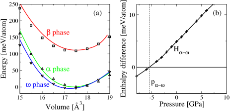
Figure 2: (color online) Fitted energies of $\alpha$, $\beta$ and $\omega$ Ti as a function of volume. (a) The MEAM potential is fit to the energy of $\alpha$, $\beta$ and $\omega$ at several volumes. The DFT results appear as symbols and the fitted MEAM curves as lines. (b) The enthalpy difference between $\alpha$ and $\omega$ as a function of pressure for MEAM. The MEAM potential predicts a transition pressure $p_{\alpha-\omega}$ of about $-5$ GPa at zero temperature similar to DFT which predicts the $\omega$ phase to be the ground state.Rudin et al. (2004)

Table 2: Fitted energies relative to the $\alpha$ phase and lattice parameters for different Ti phases within the MEAM potential and DFT calculations (in parentheses). The cohesive energy of the $\alpha$ phase is 5.171 eV/atom in GGA and 4.831 eV/atom in MEAM.

Phase	$E_{\mathrm{c}}$[meV/atom]		$V$ [Å3]		$c/a$
$\alpha$	$0$	$(0)$	$17.40$	$(17.55)$	$1.596$	$(1.583)$
$\omega$	$-5$	$(-5)$	$17.24$	$(17.28)$	$0.611$	$(0.619)$
$\beta$	$111$	$(108)$	$17.51$	$(17.34)$
fcc	$39$	$(58)$	$17.83$	$(17.53)$
A15	$54$	$(192)$	$17.99$	$(17.49)$
hexagonal	$396$	$(353)$	$17.25$	$(17.78)$	$0.982$	$(0.999)$

Predictions of the resulting potential confirm its accuracy and transferability. Table 2 compares the DFT energies and lattice parameters with the MEAM values for the experimentally observed $\alpha$, $\beta$ and $\omega$ phases and the fcc, A15 and simple hexagonal structures. The fitted MEAM values of the cohesive energy of the $\alpha$ phase of 4.831 eV and the lattice parameter of 2.931 Å agree closely with the experimental values (4.844 eV, 2.951 Å) and the DFT results (5.171 eV, 2.948 Å). For the two low-energy structures $\alpha$ and $\omega$ the final MEAM potential is also fitted to the energy as a function of volume. For $\beta$ and fcc the fit includes the equilibrium lattice constants and energies relative to hcp. For the simple hexagonal structure the potential is fitted to the energy relative to hcp for the structure with both lattice parameters fixed to the DFT values.

Table 3: Fitted elastic constants in units of GPa for $\alpha$, $\beta$ and $\omega$ Ti for the MEAM potential compared to the DFT fitting data and experiment. The MEAM potential accurately reproduces the DFT elastic constants. The experimental values for $\alpha$ Ti are measured at 4 K (Ref. Simmons and Wang, 1971) and the $\beta$ Ti elastic constants at 1238 K (Ref. Petry et al., 1991). The deviation between the calculated and measured elastic constants for $\beta$ Ti stems from the high temperature needed to stabilize the structure. For $\alpha$ and $\omega$ Ti, internal relaxations are neglected in the MEAM and DFT calculations.

	c11	c12	c44	c33	c13
— $\alpha$-phase —
MEAM	174	95	58	188	72
GGA	172	82	45	190	75
Exp.	176	87	51	191	68
— $\omega$-phase —
MEAM	191	78	48	233	64
GGA	194	81	54	245	54
— $\beta$-phase —
MEAM	95	111	53	–	–
GGA	95	110	42	–	–
Exp.	134	110	36	–	–

Table 4: Comparison of fitted point defect energies in the $\alpha$ and $\omega$ phases for the MEAM potential with DFT and three tight-binding potentials.Trinkle et al. (2006); Rudin et al. (2004); Mehl and Papaconstantopoulos (2002) The defect energies are measured relative to the corresponding $\alpha$ or $\omega$ phases at about 1 at.% defect concentration. The RMS errors of defect energies relative to GGA are given for both phases. The tetrahedral interstitial and the dumbbell-[0001] oriented along the c-axis are close in structure such that the tetrahedral defect in MEAM and GGA relaxes into the dumbbell structure. For the tight-binding potential by Rudin et al.Rudin et al. (2004) these two defects and the tetrahedral interstitial in $\omega$ collapse, an explanation and fix for this problem can be found in Ref. Trinkle et al., 2006. In the NRL potential the tetrahedral defect is unstable and relaxes to the octahedral defect.

Site	MEAM	GGA	TrinkleTrinkle et al. (2006)	RudinRudin et al. (2004)	NRLMehl and Papaconstantopoulos (2002)
— $\alpha$-defects —
Vacancy	$2.24$	$2.03$	$1.81$	$1.92$	$1.51$
Divacancy-AB	$4.00$	$3.92$	$3.82$	$3.68$	$3.73$
Octahedral	$2.64$	$2.58$	$2.89$	$2.55$	$1.31$
Tetrahedral	dumb.	dumb.	$2.86$	coll.	octa.
Dumbbell-[0001]a	$2.21$	$2.87$	$2.81$	coll.	$1.81$
RMS deviation	$0.24$	–	$0.14$	$0.16$	$0.76$
— $\omega$-defects —
Vacancy A	$2.78$	$2.92$	$2.85$	$3.25$	$2.99$
Vacancy B	$0.82$	$1.57$	$1.34$	$1.90$	$1.01$
Octahedral	$3.79$	$3.76$	$4.11$	$3.67$	$3.20$
Tetrahedral	$2.93$	$3.50$	$3.58$	coll.	$2.86$
Hexahedrala	$3.31$	$3.49$	$3.86$	$4.37$	$3.20$
RMS deviation	$0.42$	–	$0.25$	$0.5$	$0.42$

Figure 2(a) shows the result of the energy fit at different volumes for $\alpha$, $\beta$ and $\omega$. The DFT and MEAM energies agree to about 5 meV/atom with closer agreement near the energy minimum and slightly worse agreement at high compression. The MEAM potential reproduces the $\omega$ phase as the ground state and places the $\alpha$ phase slightly higher in energy by 5 meV/atom in agreement with DFT calculations.Rudin et al. (2004) Figure 2(b) shows the resulting enthalpy difference between $\alpha$ and $\omega$. At zero temperature the $\alpha$ phase transforms to $\omega$ at a pressure of $-5$ GPa in the MEAM potential.

Table 3 compares the elastic constants in MEAM with DFT results and experiment for the $\alpha$, $\beta$ and $\omega$ phases. For both methods the elastic constants are calculated neglecting internal relaxations in the $\alpha$ and $\omega$ phases. Accurate elastic constants are important for the correct description of the long-range strain fields around dislocations and other defect structures as well as in martensitic transformations. The low RMS deviation between MEAM and DFT elastic constants of 13% and maximum deviation of 29% demonstrates the quality of the fit and indicates the accuracy of the potential for the effects of strain in Ti.

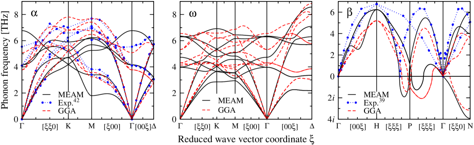
Figure 3: (color online) The phonon spectra of $\alpha$, $\beta$ and $\omega$ Ti for the classical MEAM potential (black solid lines) compared to DFT results (red dashed lines) and to experimental data for the $\alpha$ and $\beta$ phases (blue circles).Stassis et al. (1979); Petry et al. (1991) For the $\alpha$ phase the MEAM potential accurately reproduces the low energy acoustic branches reflecting the elastic constants. For optical and high-energy acoustic branches the potential reproduces the experimental phonon frequencies within 25%, generally underestimating the experimental values. Similarly for the $\omega$ phase the acoustic branches of the MEAM potential closely match the DFT results with larger discrepancies of up to 20% for the optical modes. The $\beta$ phase is mechanically unstablePetry et al. (1991) at low temperatures and transforms to $\alpha$ or $\omega$. This instability is reflected in unstable (imaginary) phonon branches in the DFT and MEAM calculations. The imaginary phonon for T-$[110]$ at the N-point corresponds to the $\beta$ to $\alpha$ transformation mechanism. The imaginary L-$\frac{2}{3}[111]$ phonon is responsible for the $\beta$ to $\omega$ transformation.

Table 4 compares the formation energies of point defects in the $\alpha$ and $\omega$ phases for the MEAM potential with DFT and several TB potentials. The defect relaxations are performed at fixed equilibrium volume for single defects in a $4\times 4\times 3$ and $3\times 3\times 4$ supercell of $\alpha$ and $\omega$, respectively. This corresponds to a defect concentration of 1%. The formation energies of the various interstitial atoms and vacancies in both phases agree well with the DFT results. In fact, the RMS errors of the energies are similar for the classical MEAM and the TB potentials. In addition the MEAM potential stabilizes the correct defects found in DFT calculations. The fitting data did not include the $\alpha$ dumbbell-[0001], the $\alpha$ divacancy-AB, or the $\omega$ hexahedral interstitial defects. The close agreement for these defects indicates the model’s accuracy.

Molecular dynamics simulations for the defects confirm their stability in MEAM. Calculations for larger simulation cells with 1080 and 1296 atoms show that the residual finite-size error of the defect formation energies is smaller than 0.1 eV. Some interstitials can lower their energy in MEAM by symmetry breaking. In the $\alpha$ phase, the octahedral interstitial moves to an off-center octahedral site with an energy 0.5 eV lower than the central octahedral site. The dumbbell cants, lowering its energy by 0.09 eV. In $\omega$ the octahedral and hexahedral interstitials reduce their energy by about 1 and 0.9 eV, respectively, moving into an off-center position. No attempt is made to determine the defect stability in DFT or TB calculations.

Experimental values for defect formation energies in Ti are rather difficult to obtain due to the presence of the $\alpha$-$\beta$ transformation and the sensitivity of diffusion to impurities such as oxygen. Based on an empirical relationship that connects the onset of positron trapping with the vacancy formation energy, positron annihilation experiments estimate for $\alpha$-Ti a value of $1.27\pm 0.05$ eV.Hashimoto et al. (1984) Isotope diffusion measurements result in diffusion activation energy of 1.75 eV.Mehrer (1990) Assuming a vacancy mechanism of diffusion, the two measurements lead to an estimate for the energy barrier of diffusion of about 0.5 eV. Both experimental values are significantly smaller than DFT predictions. The origin of the discrepancy remains unclear and beyond the scope of this paper.

The RMS force matching errors are 25% ($\beta$), 27% ($\alpha$) and 27% ($\omega$). The forces depend quadratically on the phonon frequencies, hence, the expected error in the phonons is approximately half the force-matching error and should be of the order of 15% for all three phases. Errors in the low-frequency acoustic branches are significantly less reflecting the accuracy of the elastic constants.

II.4 Accuracy of the MEAM potential

We test the accuracy of the MEAM potential by comparing the phonon spectra, surface and stacking fault energies and energy barriers for homogeneous martensitic transformations to DFT, TB and experiment.

II.4.1 Phonons

Figure 3 compares the phonon spectra obtained with the MEAM potential for the three Ti phases $\alpha$, $\beta$ and $\omega$ with the available experimental data and results from DFT calculations. For all three phases, the MEAM potential reproduces the GGA phonons within about 15%, good agreement that can be attributed to the force-matching method and fitting to elastic constants. The acoustic branches are better reproduced than the the optical modes, reflecting the accuracy of the elastic constants. Both acoustic and optical phonons are needed to describe the shuffle and strain degree of freedom in the martensitic phase transformations.

For the $\alpha$ phase the MEAM potential reproduces the overall trend of the experimental phonon branches. The optical L-[001] phonon at $\Gamma$ is 20% too high in MEAM and shows the wrong curvature away from $\Gamma$. For the K and M point, the MEAM potential underestimates the experimental phonon frequencies by about 20 to 30%.

No experimental data is available for the high-pressure $\omega$ phase. We compare the phonon spectrum for the MEAM potential with results from DFT calculations and find agreement between the MEAM potential and the DFT results comparable to that of the $\alpha$ phase with closely matching acoustic modes and larger deviations for the optical branches. In contrast to the $\alpha$ phase, for the $\omega$ phase the deviations for the optical branches are smaller and more uniform across the Brilloin zone.

The high-temperature $\beta$ phase becomes mechanically unstable at lower temperatures and shows a soft mode in the experimental data for the L-$\frac{2}{3}[111]$ phonon. The zero-temperature phonon results for the MEAM potential and DFT reflect this instability in an unstable (imaginary) phonon branch. This mode is responsible for the $(111)$ plane collapse mechanism of the $\beta$ to $\omega$ transformation. In addition, MEAM and DFT show an unstable phonon branch in the T-$[110]$ direction at the N-point which corresponds to the Burgers mechanism of the $\beta$ to $\alpha$ transformation.

II.4.2 Surface and stacking fault energies

Large changes of coordination number provide a challenging test for atomistic potentials. Specifically relevant to experiment are tests on free surfaces. Relaxations of low-index surfaces of the $\alpha$ and $\omega$ phases with MEAM and DFT determine the accuracy of the classical potential here: Calculations for increasingly larger slabs show that a slab thickness of more than 15 Å results in surface energies accurate to about 1 meV/Ų.

Table 5 compares the surface energies of the $\alpha$ and $\omega$ phases in MEAM with DFT calculations. The overall agreement of the MEAM surface energies with the DFT values for both phases is quite remarkable considering the fact that free surfaces were not used to optimize the potential. The average MEAM surface energy is about 20% too small. The good agreement encourages the potential’s application to model systems with free surfaces such as voids or cracks.

Table 5: Surface energies of the $\alpha$ and $\omega$ phase in MEAM compared to DFT calculations.

	$\alpha$			$\omega$
$\sigma$ (meV/Å2)	$[11\bar{2}0]$	$[1\bar{1}00]$	$[0001]$	$[11\bar{2}0]$	$[1\bar{1}00]$	$[0001]$
MEAM	105	97	92	98	115	116
GGA	117	153	121	152	136	133

Stacking faults in hcp materials alter the structural sequence of atomic planes in the c-direction. Their energies test the accuracy of the potential under changes of bond direction and second nearest neighbor coordination. There are three basic stacking faults possible in hcp materials. Intrinsic stacking faults $I_{1}$ and $I_{2}$ change the hcp stacking sequence $ABAB$ to $ABAB|CBCB$ and $ABAB|CACA$, respectively. Extrinsic stacking faults introduce additional layers in the hcp stacking sequence such as $ABAB|C|ABAB$. The intrinsic stacking fault $I_{2}$ describes a crystal sheared by a partial lattice vector while both the intrinsic stacking fault I₁ and the extrinsic stacking fault require a diffusive process. In hcp materials the $I_{2}$ stacking fault energy determines the dissociation of dislocation on the basal plane into partial dislocationsGirshick et al. (1998); Zaefferer (2003) and has been measured for $\alpha$-Ti.Patridge (1967)

The MEAM potential correctly predicts a metastable $I_{2}$ stacking fault with a high stacking fault energy (170 mJ/m²), though not as high as in DFT (320 mJ/m²) and experiment (300 mJ/m²).Patridge (1967) The high stacking fault energy in MEAM would result in a narrow splitting of dislocations. Elasticity predicts a splitting on the order of 7 Å (two Burgers vectors) for a basal dislocation; this is consistent with a prediction of prismatic slip, as expected for Ti.Bacon et al. (1967); Bacon and Vitek (2002) Since the MEAM potential predicts a small dislocation splitting and reproduces the elastic constants, the potential may provide an accurate description of dislocation interactions at short and long distances.

II.4.3 Energy barrier from $\alpha$ to $\omega$

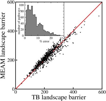
Figure 4: (color online) Comparison of energy barriers of different pathways for the $\alpha$ to $\omega$ transformation Trinkle et al. (2003, 2005) with MEAM and TB.Trinkle et al. (2006) The inset shows the distribution of the deviations between the TB and the MEAM potential. The RMS deviation is 5.5% and the maximum deviation 27% over the set of 977 pathways.

Figure 4 compares the energy barriers for different mechanism of the $\alpha$ to $\omega$ transformation in MEAM and the TB potential of Trinkle et al.Trinkle et al. (2006) The energy barrier is calculated for a two-dimensional reduced phase space for all the pathways considered in Refs. Trinkle et al., 2003 and Trinkle et al., 2005. The first degree of freedom describes the strain of the $\alpha$ cell into the $\omega$ cell and the second degree of freedom describes the shuffle motion of all atoms from their $\alpha$ to $\omega$ position within the cell. The energy barriers predicted by MEAM agree within 27% with the highly accurate TB potential by Trinkle et al.Trinkle et al. (2006) for all pathways and show an RMS deviation of only 5.5%. This excellent agreement indicates a highly accurate representation of the energy landscapes by the MEAM potential.

III Application to phases and phase transformations

The demonstrated high accuracy of the MEAM potential and its computational efficiency enable medium to large scale predictive simulations for titanium. This section presents molecular dynamics simulations for the different Ti phases and for an interface between the $\alpha$ and $\omega$ phases. The simulations determine the phase stability and pressure-temperature phase diagram of $\alpha$, $\beta$ and $\omega$ Ti and the interfacial energy and mobility for the $\alpha$–$\omega$ martensitic transformation.

III.1 Equilibrium phase diagram of titanium

Molecular dynamics simulations determine the stability of the Ti phases as a function of pressure and temperature. The simulations use the TPN (constant temperature, constant pressure, constant number) ensembleParrinello and Rahman (1982) with a time step of 1 fs. To estimate the stability range of the $\alpha$, $\beta$ and $\omega$ phases we perform molecular dynamics starting from a cubic cell of $\beta$ with 432 atoms, that is comensurate with all three phases if properly strained. For each pressure and temperature value we simulate up to 1 ns and observe the phase evolution of the system. Simulations for a solid-liquid interface containing 864 atoms estimate the melting temperature of the $\beta$ phase.

Figure 5 shows the predicted Ti equilibrium phase diagram as a function of pressure and temperature for the classical MEAM potential. At pressures below 7 GPa and temperatures below 1200 K the $\beta$ phase transforms into the $\alpha$ phase by a shear and shuffle motion of the atoms. At pressures above 8 GPa and temperatures below about 1300 K the $\beta$ phase transforms into the $\omega$ phase. The transition temperature between the $\alpha$ and $\beta$ phase is nearly independent of the pressure while the transition temperature for the $\beta$ to $\omega$ transition increases with pressure. The triple point between the $\alpha$, $\beta$ and $\omega$ phase occurs at about 8 GPa and 1200 K. At zero pressure the $\beta$ phase melts near 1900 K. The melting temperature first increases with pressure up to about 2000 K at 4 GPa and then slowly decreases with pressure.

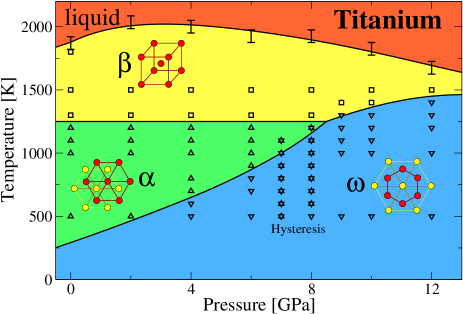
Figure 5: (color online) Equilibrium phase diagram of Ti as a function of pressure and temperature. The MEAM potential accurately describes all three solid phases, $\alpha$, $\beta$ and $\omega$, of Ti and captures the martensitic phase transformations between them. Near the triple point, the $\alpha$, $\beta$ and $\omega$ phases are nearly degenerate. As a result, whether the $\beta$ phase transforms to either $\alpha$ or $\omega$ is controlled by the initial conditions of the molecular dynamics simulations.

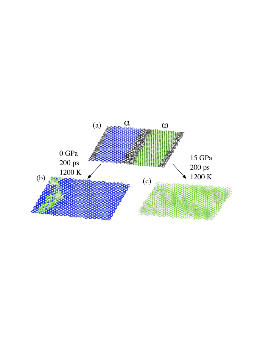
Figure 6: (color online) Molecular dynamics simulations of the $\alpha$-$\omega$ martensitic transformations. (a) The relaxed $\alpha$-$\omega$ interface is created using the TAO-1 pathway and relaxed to produce the initial interfaces. The energy for the interface is 30 meV/Ų. Unidentified atoms are colored gray, while $\alpha$ and $\omega$ atoms are colored blue and green, respectively. (b) Transformed geometry at zero compression. Molecular dynamics simulations of the relaxed interface structure at 1200 K for 200 ps transform the entire $\omega$ phase region. When the structure is fully relaxed to zero temperature, it is identified as entirely $\alpha$, except for the small region where the two interfaces merge and leave behind a number of defects. (c) Transformed geometry at 10% volume compression. The relaxed interface structure is first compressed by 10% (corresponding to $\sim$10 GPa) and then simulated at 1200 K for 200 ps. The entire $\alpha$ region transforms to $\omega$, except for a number of point defects (interstitials and vacancies). For illustration, the slab is rotated around the horizontal axis so that the $c$ axis of $\omega$ is perpendicular to the page.

The phase diagram of the MEAM potential agrees closely with experimental observations. The $\alpha$-$\beta$ transition occurs in experiment at 1155 K compared to 1250 K in the simulation. The $\beta$ phase melts at 1943K in close agreement with the MEAM value of 1900 K. Measurements of the $\alpha$-$\omega$ transformation pressure show a large hysteresis with a transformation onset ranging from 2.9 to 9.0 GPa.Bundy (1963); Zilbershtein et al. (1973, 1975); Vohra et al. (1977) The accepted equilibrium transformation pressure of $2.0\pm 0.3$ GPa was estimated from samples under shear stress that reduce the hysteresis.Zilbershtein et al. (1975) Experimental values for the triple point range from 8 GPa to 9 GPa and 900 K to 1100 K,Bandi (1966); Kutsar (1975) similar to the MEAM potential values of 8 GPa and 1200 K. The close agreement of the MEAM phase diagram with experimental data enables quantitative simulations for the martensitic phase transformations between the $\alpha$, $\beta$ and $\omega$ phases.

III.2 Pressure-induced martensitic phase transformations

Under pressure Ti transforms from $\alpha$ to $\omega$ via the TAO-1 mechanism.Trinkle et al. (2003, 2005) As a first step towards a detailed understanding of the nucleation, we simulate $\alpha$-$\omega$ interfaces under compression at finite temperature. The growth of a nucleus of a daughter phase in a parent phase is controlled by the mobility of the interface at finite temperature under a driving force. For the Ti $\alpha$ to $\omega$ martensitic phase transformation the free enthalpy difference between the two phases provides the driving force.

We construct $\alpha$-$\omega$ interfaces using the TAO-1 supercell to study the dynamics of the martensitic phase transformation. We set up interfaces between periodic slabs of untransformed TAO-1 supercells ($\alpha$ phase) and transformed TAO-1 supercells ($\omega$ phase) that minimize lattice mismatch and strain while retaining periodicity. The resulting interfaces are consistent with the pathway, minimize mismatch at the boundaries and minimize strain in each phase. The simulation cell has periodic boundary conditions in all three dimensions and contains a total of 3,600 atoms, half in each of the two phases. The system consists of alternating $\alpha$ and $\omega$ layers of 100 Å thickness. Relaxations of the initial interface estimate an interfacial energy between $\alpha$ and $\omega$ of 30 meV/Ų, roughly a third of the calculated surface energies (see Tab. 5).

All simulations are performed with OhmmsKim (2004) using a frozen cell geometry and a Langevin thermostat to produce a constant temperature of 1200 K. A time step of 1 fs is used for all numerical integration with the velocity-Verlet propagator.

Figure 6 shows the results of the molecular dynamics simulations for this cell at 1200 K. The simulations are performed at two different volumes: zero compression for the $\omega$$\to$$\alpha$ transformation corresponding to approximately 0 GPa and 15% volume compression for the $\alpha$$\to$$\omega$ transformation corresponding to about 15 GPa. At both pressures the interface between $\alpha$ and $\omega$ is mobile. At 0 GPa the system transforms completely to $\alpha$ and at 15 GPa completely to $\omega$, both within only 200 ps. In both cases the interfaces between $\alpha$ and $\omega$ approach each other and partially annihilate, leaving behind a number of interstitial and vacancy defects.

Temperature alone does not drive the transformation. We performed runs using the $\alpha$ and the $\omega$ slabs by themselves at 1200 K with no compression and 10% compression for 1 ns. In both cases the initial structure remained for the duration of the simulation. This indicates that homogeneous nucleation is not likely on the time scale of nanoseconds in cells with a few thousand atoms, while the motion of the interface does occur on such short time scale in these cells.

IV Conclusion

We developed and tested a classical potential for the complex phase transformations of the technologically important Ti system. The potential is of the modified embedded atom form ensuring computational efficiency, with parameters optimized to density functional calculations. The optimized potential describes the structure and energetics of all three phases of Ti, the $\alpha$, $\beta$ and $\omega$ phases. The elastic constants, phonon frequencies, surface energies and defect formation energies closely match density functional results even when these were not included in the fitting procedure.

Molecular dynamics simulations of the phase stability determine the potential’s equilibrium phase diagram in close agreement with experimental measurements. Simulations for the mobility of an $\alpha$–$\omega$ interface demonstrate a high interfacial mobility corresponding to the martensitic character of the $\alpha$–$\omega$ transformation. The potential enables quantitative studies of point defect evolution, grain boundary structures and mobility, as well as phase transformations in the Ti system.