The Detailed Forms of the LMC Cepheid
PL and PLC Relations
C. Koen1, S. Kanbur2 and C. Ngeow3
1 Department of Statistics, University of the Western Cape,
Private Bag X17, Bellville, 7535 Cape, South Africa
2 Department of Physics, State University of New York at Oswego,
Oswego, NY 13126, USA
3 Department of Astronomy, University of Illinois,
Urbana-Champaign, IL 61801, USA
ABSTRACT. Possible deviations from linearity of the LMC Cepheid PL and PLC relations are investigated. Two datasets are studied, respectively from the OGLE and MACHO projects. A nonparametric test, based on linear regression residuals, suggests that neither PL relation is linear. If colour dependence is allowed for then the MACHO PL relation is found to deviate more significantly from the linear, while the OGLE PL relation is consistent with linearity. These finding are confirmed by fitting “Generalised Additive Models” (nonparametric regression functions) to the two datasets. Colour dependence is shown to be nonlinear in both datasets, distinctly so in the case of the MACHO Cepheids. It is also shown that there is interaction between the period and colour functions in the MACHO data.
Key words: methods: statistical - stars: variables: Cepheids - cosmology: distance scale
1 INTRODUCTION
Cepheids are important objects in Astrophysics, both because of their use in the extra-galactic distance scale and their role in stellar evolution. Their regularly repeating light curves offer an important opportunity to test theories of stellar evolution against stellar pulsation: mass-luminosity (ML) relations mandated from evolutionary calculations can be used as input to full linear and non-linear hydrodynamic models of Cepheids and compared to observations. These ML relations contain input about evolutionary physics such as the amount of convective overshoot. Constraining theoretical models with observations can be used to gain considerable insight into evolutionary/pulsation physics. On the other hand the Cepheid period-luminosity (PL) relation has played an important role in establishing the extra-galactic distance scale and the subsequent estimation of Hubble’s constant, . The Key Project (Freedman et al. 2001) has used observations of Cepheids in a number of galaxies to estimate to within accuracy. The crucial step in this work has been the Cepheid PL relation in the Large Magellanic Cloud (LMC) which has been used to characterize a Cepheid PL relation template. This PL template has traditionally been thought to be linear, however there has also been recent work implying a variation of the slope with period in the LMC (Tammann & Reindl 2002; Kanbur & Ngeow 2004, 2006; Sandage et al. 2004; Kanbur et al. 2007a; Ngeow et al. 2005; Ngeow & Kanbur 2006a,b).
Ngeow and Kanbur (2006c) estimate the error in estimating , if a linear Cepheid PL relation is assumed and the underlying relation is ”non-linear” at a period of 10 days, and find this can lead to an error of about . Such an error seems small but with significant work being carried out to reduce zero point errors (Macri et al 2006), it is important to construct as accurate a distance scale as possible that is independent of the CMB. Further, table 2 of Spergel et al (2007) points to the fact that an independent estimate of , accurate to less than , will help to break the degeneracy between and present from WMAP CMB studies. An independent estimate of accurate to will result in a reduction of the confidence interval on by almost a factor of two over that with WMAP data alone.
In previous studies, a rigorous statistical test, the test, was applied to the LMC Cepheids to test for the linear versus non-linear PL relation. Here by “non-linear” we mean two lines of significantly differing slope which are continuous at a period of 10 days. The test results that were obtained from the OGLE (Optical Gravitational Lensing Experiment, Udalski et al. 1999) and MACHO Cepheid data, in Kanbur & Ngeow (2004; 2006) and Ngeow et al. (2005) respectively, strongly imply that the LMC PC/PL relations are non-linear. It is important to note that several other statistical tests, such as the tests, least absolute deviation, robust estimation and loess procedures, were also applied to the MACHO data, and these results also point to a non-linear LMC PL relation (Ngeow et al. 2005). Recently, Kanbur et al (2007a) developed the use of testimators and a likelihood based method using the Schwarz Information Criterion, to study non-linearities in the LMC PL relation (using both OGLE and MACHO Cepheid data) and again came to the same conclusion: the LMC Cepheid PL relation is non-linear in the sense described above. The test also suggested that the LMC period-colour (PC) relation is non-linear, in contrast to the Galactic and SMC (Small Magellanic Cloud) PC relations (Kanbur & Ngeow 2004). Since the question of the non-linearity of the LMC PL relation is important in distance scale and stellar studies, it is vital to establish this as firmly as possible; this is one of the motivations for this paper.
In addition to investigating the non-linearity of the LMC PL relation, we also study the LMC period-luminosity-colour (PLC) relation. A number of authors, including Sandage (1958) and Madore and Freedman (1991) have derived the Period-Luminosity-Color (PLC) relation and shown how it arises from the period-mean density theorem, the Stefan-Boltzmann law and the existence of an instability strip. These authors also point out that the PL/PC relations are obtained from the PLC relation by averaging over the variable not included in the relation.
In Section 2, we briefly describe the data used in our study. In Section 3 we apply a preliminary test study on the LMC PL relation. This is followed by more detailed analysis in Section 4, based on a non-parametric model fitting procedure. An extension to the PLC relation is presented in Section 5. The conclusion and discussion of our results are given in Section 6.
We add a few sentences on the use of non-parametric methods in what follows. The term “non-parametric” is actually used in three slightly different senses. First, the major innovation (sections 4 and 5) in this paper is the use of “non-parametric regression”. The meaning is not necessarily the usual one of “distribution-free”: rather, it means that the form of the regression is not specified – the regression function is “unstructured”, being dictated by the data itself. Of course, this flexibility allows one to detect subtleties which may otherwise be overlooked. Second, in the next section of the paper we use a well-known distribution-free statistic, the “Wald-Wolfowitz runs test”. This non-parametric statistic uses only data ranks, and hence typically not very powerful. Third, also in the next section use is made of a permutation method. This avoids distributional assumptions about the data, by using re-orderings of the data itself to establish significance levels.
2 THE DATA
We use two sets of LMC Cepheid data in our study. The first data set is the extinction corrected -band mean magnitudes and colours for the OGLE LMC Cepheids taken from Kanbur & Ngeow (2006), supplemented with additional Cepheids from Sebo et al (2002), and referred as “OGLE” data in this paper. The second data set is the MACHO Cepheids data, with extinction corrected mean magnitudes and colours, adopted from Ngeow et al (2005). Using these two data sets allow us to compare the results, particularly for the different photometric filters used.
A possible complication is that any apparent non-linearity in PL or PLC relations could be caused by extinction errors which are a function of colour or period. Arguments against extinction errors as a cause of observed non-linear LMC PL and PC relations were presented in Kanbur & Ngeow (2004), Kanbur & Ngeow (2006), Kanbur et al. (2007b), Ngeow et al. (2005), Ngeow & Kanbur (2006b) and Sandage et al. (2004), and will therfore not be repeated in detail here. In particular, a possible period dependency of extinction errors has been investigated in Ngeow & Kanbur (2006b). If such extinction errors were present, then the PC relations at maximum light would be such that LMC Cepheids would get hotter at maximum light as the pulsation period increases: a fact which would be hard to reconcile with pulsation theory especially as Galactic Cepheids, in common with LMC Cepheids, display a flat PC relation at maximum light (Kanbur & Ngeow 2004, 2006). Further, the dependence of extinction error on colour would need to be very complicated to explain both the non-linearity at mean light whilst preserving the flatness at maximum light.
It is also noted that the reddening values adopted here are the same as those used in many distance scale studies (Freedman et al. 2001).
3 A PRELIMINARY INVESTIGATION BASED ON A TEST PROCEDURE
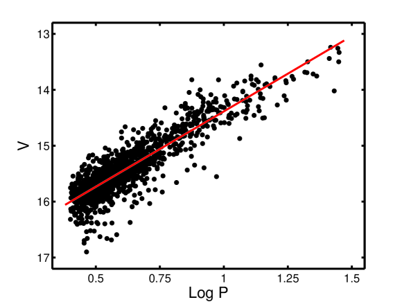
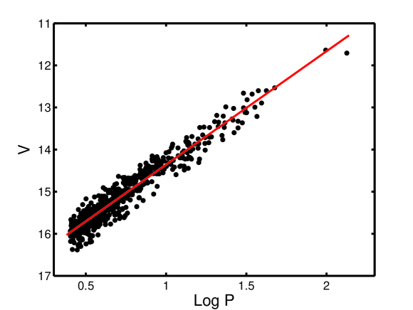
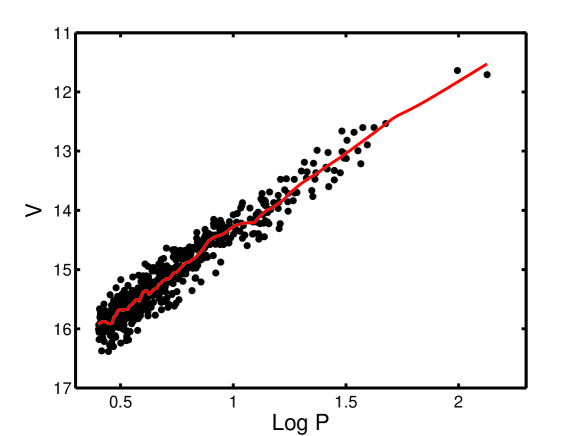
Figs. 1 and 2 show the MACHO and OGLE PL data, with least squares linear fits of the form
| (1) |
For the sake of completeness,
| (2) |
where standard errors of coefficient estimates are given in brackets. Although both fits are excellent, it is nonetheless of some interest whether there may be subtle deviations from the strictly linear relations between and shown by the lines: although this may have little importance for prediction of luminosity given the period, it could (e.g.) have an important bearing on the modelling of Cepheid pulsations.
A simple procedure which provides some insight into the problem is to study partial sums of the residuals of the least squares fits. First arrange the data so that the period values are in ascending order:
where is the sample size. Then
| (3) |
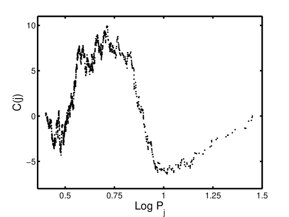
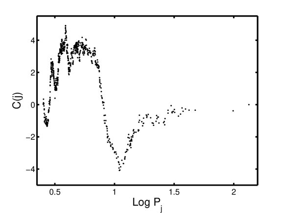
are the partial sums of the residuals . If there are no deviations from linearity, then is the sum of uncorrelated random numbers and hence a simple random walk. However, if there are deviations from linearity successive residuals may be correlated, and hence will not be a simple random walk. Partials sums of the can be seen in Figs. 3 and 4.
A statistic which can be used for testing whether the partial sum is a pure random walk is its vertical range
this may be expected to be inflated by positively correlated residuals. Significance levels for the values of are readily obtained by permutation, as follows:
-
(i)
Permute the ; this will randomise the residuals by destroying any possible trends.
-
(ii)
The partial sums of the permuted will be true random walks – find the statistic for the permutation.
-
(iii)
Repeat steps (i) and (ii) a large number of times, noting the values of .
-
(iv)
Determine the fraction of permutation -values which exceeds the observed value – this estimates the significance level of the observed .
Applying 10000 permutations, significance levels of 3% and 4% were obtained for the MACHO and OGLE data respectively, suggesting meaningful deviation of the observed from randomness. The implication is therefore that the PL relation is not perfectly linear.
Study of Figs. 3 and 4 shows that there is an excess of positive residuals for and , and an excess of negative values for .
Interestingly, application of the standard Wald-Wolfowitz runs test (e.g. Conover 1971) for randomness of the residuals gives conflicting results for the two datasets – significance levels of 45% and 0.9% for the OGLE and MACHO data respectively. Of course, the procedure uses only the signs, and not the sizes, of the .
It is known that Cepheids follow a PLC, rather than simply a PL, relation. It may therefore be prudent to replace (1) by
| (4) |
where indicates a colour index, with regression coefficient . This has a substantial influence on the significance levels of the statistic : for the OGLE data is increases to 33%, while the level for the MACHO data is reduced to 0.7%. The corresponding Wald-Wolfowitz test levels are 43% and 1.5%.
To summarise, there is strong evidence of non-randomness in the residuals of the MACHO data, both for the PL and the PLC relations. For the OGLE data the results are ambiguous.
4 PL RELATION
An alternative to the imposition of a fully specified parametric model such as (1) is to allow the form of the regression to be dictated by the data. The idea is conveniently illustrated by a technique known as “loess” (see e.g. Cleveland & Devlin 1988). Ngeow et al (2005) initially used this method on MACHO data and found a similar result to that reported here. Here we study it in more detail and apply it to both MACHO and OGLE Cepheid data. The method entails fitting a low order polynomial (in the present case a straight line) over restricted sections (“windows”) of the data by weighted least squares. In the implementation here the only free parameter is the width of the window, which is usually given as a fraction of the range of the independent variable (i.e. ) . The smaller the more “local” the estimated regression, and the more detail it shows. Fig. 5 shows a loess regression of the OGLE data, using ; if is increased towards unity the loess regression resembles the linear fit of Fig. 2.
A key element is then obviously the choice of window width , and it is desirable to use an objective method to find it. This is readily done by “cross-validation”:
-
(i)
Choose a value of the window width .
-
(ii)
Leave out the first datapoint and obtain a loess estimate of the magnitude by fitting the regression to the remaining data.
-
(iii)
Note the discrepancy
between the true and predicted values.
-
(iv)
Repeat steps (ii)-(iii) for the second, third,…, last datapoints, giving the set of discrepancies.
-
(v)
The value of the cross-validation criterion for the value of from (i) is the defined as
(5) Clearly, it evaluates the predictive power over all the observations of the loess fit based on the particular value of .
-
(vi)
Repeat steps (i)-(v) for all candidate values of .
-
(vii)
The optimal is that which minimises .
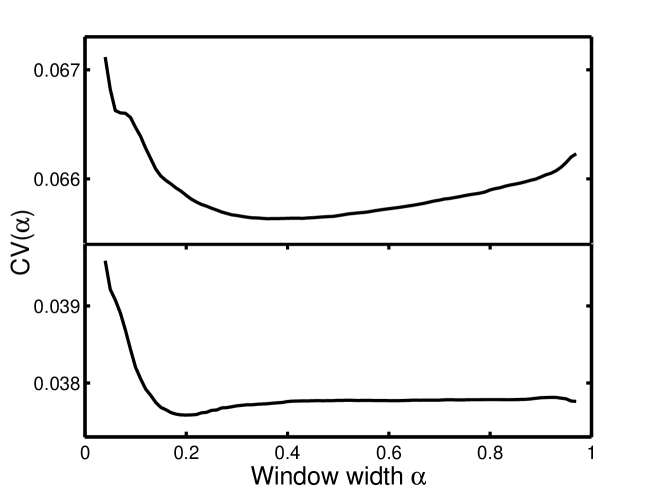
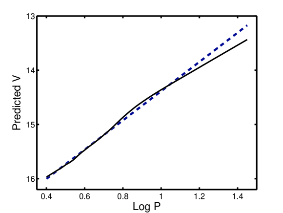
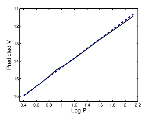
The cross-validation functions for the two datasets are plotted in Fig. 6; optimal window widths are 0.36 and 0.20 respectively for the MACHO and OGLE observations. In Figs. 7 and 8 the resultant loess functions are compared to the regression lines from (1). A small difference between the curves over the approximate interval is visible in both diagrams. There is also a substantial disagreement at the longest periods for the MACHO results in Fig. 7: this is clearly due to the systematic difference between the data and the linear regression line for (see Fig. 1). Similarly, the slight divergence between the loess and linear regression lines at the longest periods in Fig. 8, can be traced to the influence of the two OGLE datapoints with (see Fig. 2).
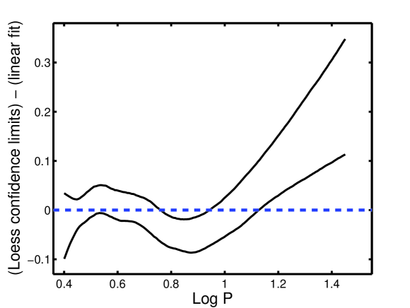
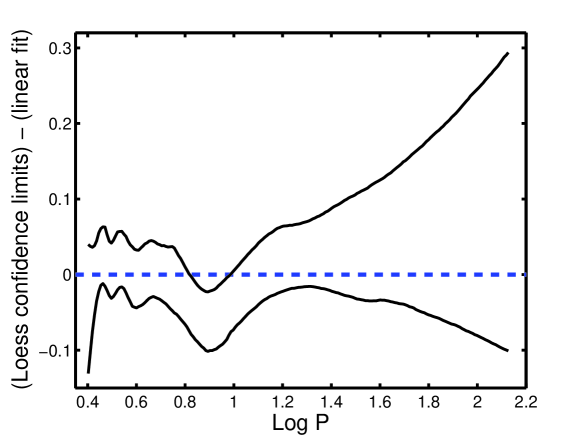
The question arises as to whether the discrepancies between the loess curves and the straight line fits are at all meaningful. In order to address this issue confidence intervals for the loess curves are estimated by bootstrapping (e.g. Efron & Tibshirani 1993). The results, based on 5000 bootstrap samples, are plotted in Figs. 9 and 10. Rather than showing the linear regression line and the 95lower limits, the difference between the linear fit and the confidence limits are plotted, in order to more clearly display the deviations. It is notable that the linear fits lie outside the confidence intervals for the loess functions for roughly. This supports previous work which has suggested a ”break” around a period (Kanbur & Ngeow 2004, Ngeow et al 2005, Kanbur et al 2007a).
The R software add-on package “mcgv” contains an alternative nonparametric regression facility in the form of thin plate regression splines (TPRS) (e.g. Wood 2006). The form of cross-validation used is based on a balance between the sum of squared model residuals (which measures the goodness of the model fit) and a smoothness term. Cross-validation in mcgv is automated.
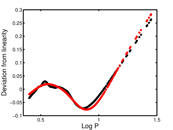
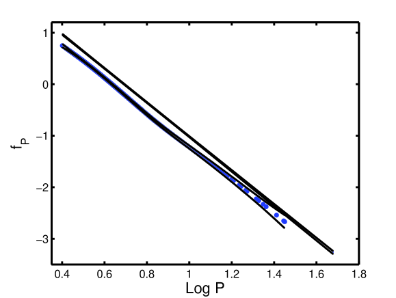
The loess and TPRS results are compared for the MACHO and OGLE respectively in Figs. 11 and 12. The agreement is very good – in particular, the deviations from linearity for are also evident in the TPRS results. Despite the fact that more effective degrees of freedom are required for the nonparametric fits (6.41 and 8.71 for the TPRS fits to the MACHO and OGLE data respectively) than for linear regression (3 degrees of freedom), the former fits follow the data considerably more closely. Model selection tools such as the “Akaike Information Criterion” (AIC, e.g. Burnham & Anderson 2002) can be used to test whether the improved model fit warrants the additional degrees of freedom expended. In this case, the TPRS fits are both preferred by very wide margins.
5 PLC RELATION
Unusual datapoints can have substantial, often somewhat distorting, influences on regression surfaces. It is therefore worthwhile examining the datasets carefully in order to identify such data. This is most easily done using ordinary multiple linear least squares regression.
Fitting PLC relations to the two datasets give the results
| (6) |
with residual standard deviations 0.164 and 0.097 mag. Regression diagnostics were examined in order to identify observations which gave rise to large residuals and/or were unduly influential on parameter estimates. “Cooks’s ” statistic was used for the latter purpose – see e.g. Montgomery, Peck & Vining (2001) (or almost any other modern text devoted to linear regression theory). Three points were eliminated from the MACHO data, and four from the OGLE data, on the basis of these diagnostics. The PLC relations were then re-estimated for the reduced datasets, and the new sets of diagnostics examined. This led to a further two deletions from the OGLE data. The final results, replacing (6), are
| (7) |
with residual standard deviations of 0.162 and 0.074 mag. The substantial reduction in residual variance, and large changes in regression coefficients for the OGLE results are particularly striking.
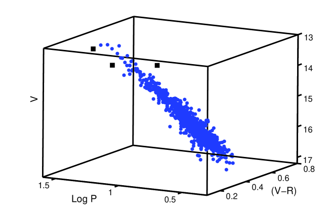
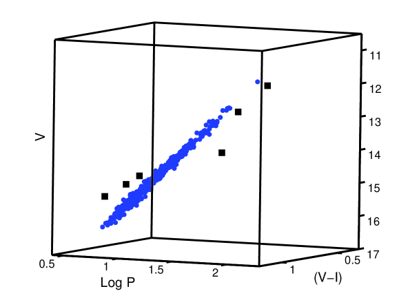
It is interesting to examine the positions of the rejected observations in three-dimensional dataplots. The plots in Figs. 11 and 12 were obtained by selecting perspectives which clearly show the positions of all questionable data. It is clear the observations for each dataset lie close to a plane, and that points with unsatisfactory regression diagnostics (marked by squares) all deviate from the plane. The fact that the plane in Fig. 12 (OGLE data) is so well-defined explains why removal of the outlying points made such a substantial difference to the estimated coefficients. In the remainder of this paper we work with the reduced datasets ( for MACHO and OGLE data respectively). Note that one high-influence datum in the OGLE data is retained (for the brightest Cepheid – see Fig. 12), since its associated residual is very small, and since its omission has very little influence on the values of the three estimated parameters.
An obvious extension of the linear PLC relation to the nonparametric case is the so-called “Generalised Additive Model”
| (8) |
where is a constant; denotes a colour index; and and are nonparametric regression functions such as loess or TPRS fits. Due to the several attractive features (automated cross-validation, to mention but one) the R add-on package is once again used to perform TPRS fits of (8) to the data.
The results can be seen in Figs. 15 and 16. The estimated for the OGLE data is linear: the effective degrees of freedom, 1.00, confirms this. By implication the model (8) reduces to
| (9) |
Not surprisingly, the AICs of models (8) and (9) are exactly equal for the OGLE data.
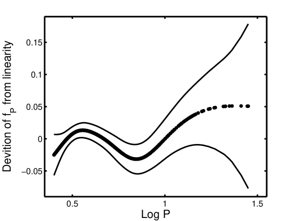
The function for the MACHO data shows the familiar deviation from linearity in the range ; this is more clearly demonstrated in Fig. 17, where a linear fit to has been subtracted.
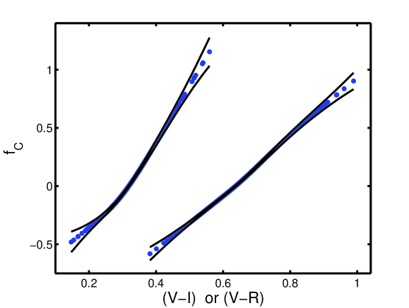
Inspection of the functions in Fig. 16 shows that both are distinctly nonlinear.
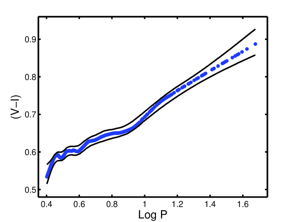
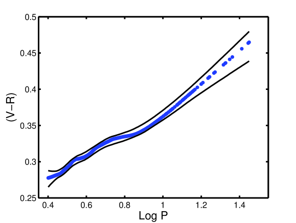
It is of obvious interest to investigate why reduces to the perfectly linear form in the case of the OGLE data, when the dependence of on in the PL relation is nonlinear. Examining the relationship between and the colour index gives some insight into this question. The results of a loess regression of on for the OGLE data are displayed in Fig. 18. The 95% confidence intervals, obtained from 5000 bootstrap samples, are also shown. Calculations were done using a smoothing window of width 0.20, as indicated by cross-validation. The analogous plot for the MACHO data, based on a smoothing window width of 0.33, is in Fig. 19. In the case of the OGLE data there is a clear change in the relationship between and in the neighbourhood . It appears that small deviations from linearity in the relation in Fig. 8 are compensated by the colour dependence. In the case of the MACHO data the kink in the plot (Fig. 19) is of similar size to that in Fig. 18, but the deviation from linearity in the plot is larger (Fig. 7). This may explain why the function remains nonlinear in the case of the MACHO relation. These results support similar work presented in Kanbur and Ngeow (2004) and Ngeow and Kanbur (2005) on the non-linearity of the LMC PC relation using tests, and on the linearity of the LMC Wessenheit function.
Nonparametric regression lends itself to much more flexible forms than ordinary multiple regression. Two possible alternatives to (8) are
| (10) |
and
| (11) |
which allows for interaction between the two independent variables.
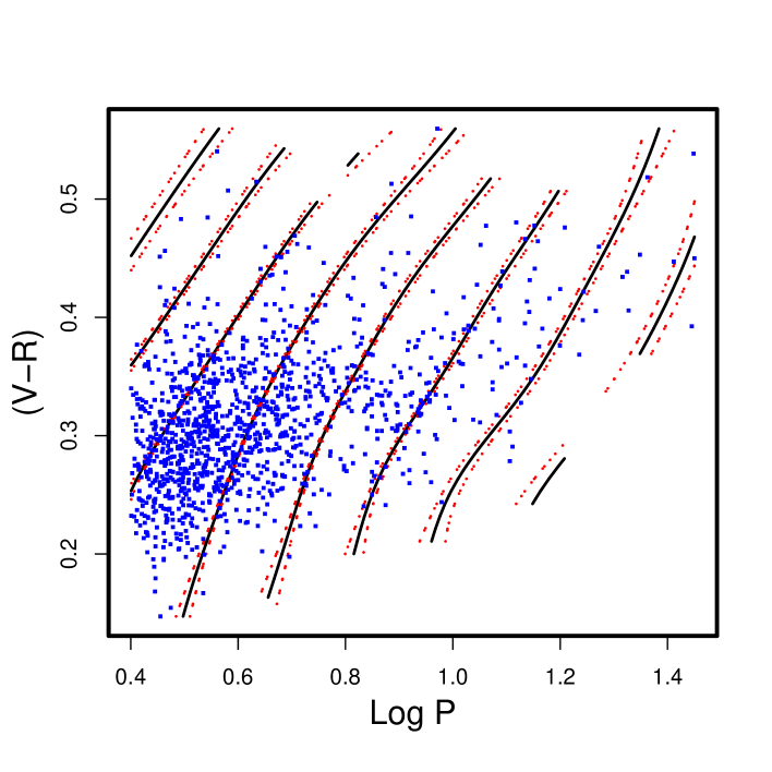
The two Generalized Additive Models (10) and (11) were also fitted to both datasets. For the OGLE data, the AIC-preferred model is (10), but a more detailed analysis (ANOVA) shows that the contribution from the interaction function is not significant – hence the model effectively reduces to (8). For the MACHO data the pure interaction model (11) is preferred, with (10) the second choice. According to the AIC, the additive model (8) is a very distant third choice. A contour plot of the fit of the model (11) can be seen in Fig. 20 – this demonstrates why (8) is inadequate. Of course, in practice (11) would be more tedious to work with than the simpler additive form (8).
A few words of explanation of Fig. 20 may be in order. The form of a purely linear PLC relation would of course be
One way of displaying this graphically would be to draw the lines
in the - plane, for various values of the constant. The equations describing these contour lines are
i.e. straight lines with slope . Fig. 20, the equivalent for the non-parametric function , shows not only that the relations are nonlinear, but also that there is “interaction” – the form of the relation depends on the region of the – plane it inhabits.
6 CONCLUSIONS & DISCUSSION
It should perhaps come as no surprise that with the acquisition of large amounts of new data finer detail in the relationships between astrophysical observables are uncovered. The best-fitting models of the two datasets are given by (11) (MACHO) and (9) (OGLE) respectively, which both are both nonlinear.
Estimates of the effect of such small non-linearities on the Cepheid distance scale and on Hubble’s constant are given in Ngeow and Kanbur (2006c) and amount to . Such an error seems small but in the era of ”precision cosmology” with a drive toward a distance scale accurate to , such an effect is important. Perhaps just as important, a proper characterization of the precise detail in the observed phenomena will assist in placing improved constraints on pulsation models of Cepheids and in particular on their ML relations, and hence on details of stellar evolutionary physics such as the amount of convective core overshoot.
A possible physical explanation for this non-linearity is outlined in the papers by Kanbur et al. (2004), Kanbur & Ngeow (2006) and Kanbur et al. (2007b), which studied Galactic, LMC and SMC Cepheid models respectively. Briefly, these papers suggest the non-linearity is caused by the interaction of the hydrogen ionization front (HIF) and photosphere and the way this interaction varies with period. At low densities, if the HIF and photosphere are engaged (i.e. the photosphere lies at the base of the HIF) then the temperature of the photosphere and hence the colour of the star are almost independent of global stellar properties such as the period. Since the relative location of the photosphere and HIF varies with the ratio, and since this varies with period, modelling has implied that for LMC Cepheids with a period greater than 10 days, the photosphere and HIF are not engaged. Thus these stars have a different PC relation than their shorter period counterparts, Because the PC and PL relations are really forms of the PLC relation, then a change in the PC relation results in a change in the PL relation. Galactic Cepheids are such that the HIF-photosphere interaction only really occurs at maximum light at low densities. LMC Cepheids are such that this HIF-photosphere interaction starts to occur at low densities only for Cepheids with periods greater than 10 days. SMC Cepheids are such that this HIF-photosphere interaction always occurs at high densities (Kanbur et al. 2004; Kanbur & Ngeow 2006; Kanbur et al. 2007b).
ACKNOWLEDGMENTS
The authors are grateful for the efforts of those who have developed and maintained the R statistical software. SMK acknowledges support from a small research grant from the American Astronomical Society and the Chretien International research grant. CN acknowledges financial support from NSF award OPP-0130612 and a University of Illinois seed funding award to the Dark Energy Survey.
REFERENCES
Burnham K.P., Anderson D.R., 2002, Model Selection and Multimodel Inference: a Practical Information-Theoretic Approach (Second Edition). Springer, New York
Cleveland W.S., Devlin S.J., 1988, J. Amer. Stat. Assoc., 83, 597
Conover W.J., 1971, Practical Nonparametric Statistics. John Wiley & Sons Inc., New York
Efron B., Tibshirani R.J., 1993, An Introduction to the Bootstrap. Chapman & Hall, London
Freedman, W., et al., 2001, ApJ, 553, 47
Kanbur, S. & Ngeow, C., 2004, MNRAS, 350, 962
Kanbur, S. & Ngeow, C., Buchler R., 2004, MNRAS, 354, 212
Kanbur, S. & Ngeow, C., 2006, MNRAS, 369, 705
Kanbur, S., Ngeow, C., Nanthakumar, A. & Stevens, R., 2007a, PASP, 119, 512
Kanbur S., Ngeow C., Feiden G., 2007b, submitted
Macri L., Stanek K., Bersier D., Greenhill L., Reid M., 2006, ApJ, 652, 1133
Madore B., Freeman W., 1991, PASP, 103, 933
Montgomery D.C., Peck E.A., Vining G.G., 2001, Introduction to Linear Regression Analysis (Third Edition). John Wiley & Sons, Inc., New York
Ngeow, C. & Kanbur, S., 2005, MNRAS, 360, 1033
Ngeow, C., Kanbur, S., Nikolaev, S., Buonaccorsi, J., Cook, K. & Welch, D., 2005, MNRAS, 363, 831
Ngeow, C. & Kanbur, S., 2006a, MNRAS, 369, 723
Ngeow, C. & Kanbur, S., 2006b, ApJ, 650, 180
Ngeow, C. & Kanbur, S., 2006c, ApJ, 642, L29
Sandage, A., 1958, ApJ, 127, 513
Sandage, A., Tammann, G. A. & Reindl, B., 2004, A&A, 424, 43
Sebo, K., et al., 2002, ApJS, 142, 71
Spergel D., et al., 2007, ApJ, in press (ArXiv:astro-ph/0603449)
Tammann, G. A. & Reindl, B., 2002, Astrophys. & Space Sci., 280, 165
Udalski, A., Soszynski, I., Szymanski, M., Kubiak, M., Pietrzynski, G., Wozniak, P., & Zebrun, K. 1999, Acta Astron., 49, 223
Wood S., 2006, Generalized Additive Models. An Introduction with R. Chapman & Hall/CRC, Boca Raton (Fl)