IBM-1 description of the fission products ^108,110,112Ru

Abstract

IBM-1 calculations for the fission products ^108,110,112Ru have been carried out. The even-even isotopes of Ru can be described as transitional nuclei situated between the U(5) (spherical vibrator) and SO(6) ($\gamma$-unstable rotor) symmetries of the Interacting Boson Model. At first, a Hamiltonian with only one- and two-body terms has been used. Excitation energies and $B$(E2) ratios of gamma transitions have been calculated. A satisfactory agreement has been obtained, with the exception of the odd-even staggering in the quasi-$\gamma$ bands of ^110,112Ru. The observed pattern is rather similar to the one for a rigid triaxial rotor. A calculation based on a Hamiltonian with three-body terms was able to remove this discrepancy. The relation between the IBM and the triaxial rotor model was also examined.

, , , , , , , , , ,

1 Introduction

In recent years neutron-rich even-even isotopes of Ru have been studied by gamma-ray spectroscopy. In this work we will concentrate our attention on the heavy fission products ^108,110,112Ru, for which new data are available. In most cases, such nuclei were produced by spontaneous fission, and the gamma-rays were studied by using large Ge-detector arrays [1, 2, 3]. Recently, fission products with masses between about 100 and 112 were produced by a ²⁵²Cf source, and studied with the Gammasphere array [4, 5, 6]. In the most recent publication from the latter collaboration, Zhu et al.  [7], several new excited states and transitions have been reported. Some neutron-rich even-even Ru isotopes were also produced by the $\beta$-decay of Tc [8, 9, 10, 11]. Recently, ¹⁰⁴Ru was reinvestigated by Coulomb excitation [12].

The impressive accumulation of experimental data during the last 5-6 years has created improved conditions for revisiting the description of ^108,110,112Ru by means of nuclear models. In the paper by Stachel et al. [13] the authors proposed to consider the isotopes between ⁹⁸Ru and ¹¹⁰Ru as belonging to a transition from the U(5) to the SO(6) limit of the Interacting Boson Model (IBM) [14]. In geometrical terms this would be equivalent to a transition between a spherical vibrator [15] and a $\gamma$-unstable rotor [16]. The authors of [13] used a schematic Hamiltonian, which can describe the main features of the U(5) to SO(6) transition in even-even Ru isotopes. In their conclusion they viewed this simplified treatment only as a guideline. A more detailed approach is necessary for a comparison of the data with the model for each nucleus. Even-even Ru isotopes were studied in [17, 18], where the IBM-2 was used. In this variant of the model, separate proton and neutron bosons are considered. The authors focussed their attention on mixed-symmetry states [19, 20, 21].

More recently a search for a possible phase transition in these nuclei was carried out in [22]. Again, a schematic Hamiltonian was used to describe the U(5) to SO(6) transition. The use of coherent states [23, 24] allowed the authors to keep track of the dependence on deformation of the total energy surface. The authors came to the conclusion that a phase transition takes place at ¹⁰⁴Ru, which can be considered as an example of the E(5) critical symmetry proposed by Iachello [25].

Other models have also been used for the calculation of excitation energies and transition strengths. The Rotation-Vibration Model [4, 26] and the Generalized Collective Model [27, 28] were applied to ^108-112Ru. A microscopically based Quadrupole Bohr Hamiltonian was applied to ¹⁰⁴Ru [12].

Recently excited states in ^109-112Ru were populated in a ${}^{238}{\rm U}(\alpha,{\rm f})$ fusion-fission reaction [29]. The bands above the backbending were interpreted with the cranked shell model.

The main aim of this work is to describe the most important observables of the heavy ^108,110,112Ru isotopes such as excitation energies, E2 branching ratios and the odd-even staggering in the quasi-$\gamma$ bands by using the Interacting Boson Model. We will use both the standard IBM-1 Hamiltonian and an extended one, which also comprises a three-body term. We will also discuss the relation between the IBM-1 and the Rigid Triaxial Rotor Model (RTRM). The calculations will be compared to the latest experimental information presented in [7] which includes revisited $\gamma$-ray intensities and, for ^110,112Ru, a newly observed band-like structure built on the proposed (4${}^{+}_{3}$) state.

2 The model

2.1 The standard IBM-1

If we examine the systematics of excitation energies in even-even ^96-112Ru, we clearly see a transition between two well-known patterns. In the light Ru isotopes, e.g. ^96,98Ru, the excitation energy ratio $R_{4/2}=E(4_{1}^{+})/E(2_{1}^{+})\approx 2$. With increasing neutron number, $E(2_{1}^{+})$ decreases, thus indicating an increase of collectivity; the heaviest isotopes ^110,112Ru have $R_{4/2}\approx 2.7$, a quite typical value for SO(6)-type nuclei. In the light Ru isotopes we observe the two-phonon-triplet $4^{+},2^{+},0^{+}$. Together with the energy ratio $R_{4/2}$, these are characteristic features of a spherical vibrator. At the other extreme, the $0^{+}_{2}$ state (if observed) is closer to the $3^{+}_{1}$ state, and it looks like belonging to a $6^{+},4^{+},3^{+},0^{+}$ multiplet, as predicted by the Wilets-Jean model [16] or the SO(6) symmetry of the IBM. The energy ratios fit into the picture too. This is a good reason for trying to describe the even-even Ru isotopes in the framework of the algebraic IBM-1.

The building blocks of the IBM-1 are $d$-bosons with an angular momentum 2, and $s$-bosons, with an angular momentum 0. The corresponding creation (annihilation) operators are $d^{{\dagger}}(d)$ and $s^{{\dagger}}(s)$, respectively. A nucleus is characterized by the total boson number $N$, which is equal to half the number of valence nucleons (particles or holes). No distinction is made between proton and neutron bosons.

A very important feature of the IBM is the conservation of the total number of bosons. The operator $\hat{N}=\hat{n}_{d}+\hat{n}_{s}$, where $\hat{n}_{d}$ and $\hat{n}_{s}$ are the $d$-boson and $s$-boson number operators, commutes with the Hamiltonian and with the operators of electromagnetic transitions. The boson number varies along the ⁹⁸Ru to ¹¹²Ru chain from $N=5$ to $N=10$.

It can be shown [14] that the 36 linearly independent boson one-body operators are the generators of a Lie algebra of the unitary group U(6). A Casimir operator is defined by the condition that it commutes with all elements of the algebra.

A fundamental concept of the IBM is the existence of dynamical symmetries (DS), which assumes the existence of a chain of subalgebras (subgroups) starting from U(6) and ending at SO(3). In a DS the Hamiltonian is a linear combination of Casimir operators belonging to a chain of subalgebras. We first consider the U(5) subalgebra chain

$${\rm U}(6)\supset{\rm U}(5)\supset{\rm SO}(5)\supset{\rm SO}(3).$$ (1)

The quantum numbers of the chain (1) are the total number of bosons $N$, the number of $d$-bosons $n_{d}$, the $d$-boson seniority $\tau$ and the angular momentum $L$. The main quantum number is $n_{d}$. The label $\tau$, associated with SO(5), here represents the number of d-bosons which are not coupled pairwise to angular momentum zero. An additional quantum number $\nu_{\Delta}$ is necessary in order to specify completely the reduction from SO(5) to SO(3). This quantum number is related to the number of triplets of $d$-bosons coupled to angular momentum zero.

Besides the U(5) chain, there are two other possibilities, namely SU(3) and SO(6). We mentioned already that the heavy Ru isotopes have properties which closely resemble those of the SO(6) symmetry. The corresponding subalgebra chain is

$${\rm U}(6)\supset{\rm SO}(6)\supset{\rm SO}(5)\supset{\rm SO}(3).$$ (2)

The algebra U(5) does not belong to this chain and, as a consequence, the number of $d$-bosons $n_{d}$ is not a good quantum number. On the other hand, due to the presence of SO(5), the $d$-boson seniority $\tau$ is again a good quantum number.

The “standard” IBM-1 Hamiltonian contains only one- and two-body operators. The excitation spectrum of a single nucleus (at fixed total boson number $N$) depends on a maximum of six free parameters in the Hamiltonian. A less general Hamiltonian which is suitable for the description of the transition between the U(5) and SO(6) DS is [30]

$$\hat{H}=\epsilon\hat{n}_{d}+\kappa\hat{Q}^{\chi}\cdot\hat{Q}^{\chi}+2\lambda\hat{L}\cdot\hat{L}+\beta\hat{n}_{d}^{2},$$ (3)

where $\hat{Q}^{\chi}$ is the quadrupole operator. Its components are

$$\hat{Q}_{\mu}^{\chi}=[d^{\dagger}\times s+s^{\dagger}\times\tilde{d}]^{(2)}_{\mu}+\chi[d^{\dagger}\times\tilde{d}]^{(2)}_{\mu}$$ (4)

where $\times$ denotes tensor coupling. The effect of the $\beta\hat{n}_{d}^{2}$ term with $\beta<0$ is an increase of the moment of inertia with increasing spin (or $\tau$). This so-called “$\tau$-compression” has been first used in [31].

The electric quadrupole transition operator is defined as

$$\hat{T}_{\mu}({\rm E2})=q\left([d^{\dagger}\times s+s^{\dagger}\times\tilde{d}]^{(2)}_{\mu}+\chi[d^{\dagger}\times\tilde{d}]^{(2)}_{\mu}\right),$$ (5)

where $q$ is an effective quadrupole charge.

In the consistent-$Q$ formalism [32] the parameter $\chi$ in $\hat{T}({\rm E2})$ has the same value as in the Hamiltonian. If $\chi=0$, the E2 selection rule is $\Delta\tau=\pm 1$; if $\chi\neq 0$, E2 transitions with $\Delta\tau=0,\pm 2$ are also allowed. For $\chi=0$, $\tau$ is a good quantum number for the entire U(5) to SO(6) transition [33]. In this case the wave functions have an important property. For a given value of $\tau$, $n_{d}$ can have only the values $\tau,\tau+2,\tau+4$, etc. In the U(5) limit this reduces to a fixed value of $n_{d}$.

The Hamiltonian (3) displays a U(5) DS if $\kappa=0$ and, in this case, its excited states will be those of an anharmonic vibrator. If, on the contrary, we want to obtain an SO(6) DS, the parameters $\epsilon$, $\chi$ and $\beta$ must vanish. If we examine the level schemes of the even-even Ru isotopes, we notice that none of them is entirely consistent with either the U(5) or the SO(6) symmetry.

In order to carry out a quantitative comparison of the data with the theoretical predictions, the Hamiltonian (3) must be diagonalized numerically. This has been done by using the program PHINT [34]. The actual fitting procedure makes use of a fast graphical user interface [35]. Its input contains the parameters used in eq. (3).

As it will be shown in sect. 3, most properties of the investigated nuclei can be correctly described by the relatively simple Hamiltonian (3). However, the odd-even staggering in the quasi-$\gamma$ bands of ^110,112Ru does not look like the pattern we should expect for SO(6)-type nuclei. In this symmetry, in a first approximation, the states belonging to a $\tau$-multiplet are degenerate. If we switch on the term in $\hat{L}^{2}$, this degeneracy is lifted, and the states with higher $L$ are raised in energy. Since this contribution from SO(3) is small, this will result in a slight lowering of the states with odd angular momenta with respect to those with even angular momenta. This behaviour has been observed in most SO(6)-type nuclei, including ¹⁰⁸Ru. There are a few SO(6) type nuclei in which this odd-even staggering is replaced by a pattern which is closer to the RTRM. In the latter case, for example, the $5^{+}_{1}$ state is nearer to $4^{+}_{2}$ than to $6^{+}_{2}$, as it would be required by the IBM-1 [36] with only two-body terms in the Hamiltonian. It has been observed that in the quasi-$\gamma$ bands of ^110,112Ru, the odd-even staggering is closer to the RTRM [37]. We will see in the next subsection that this discrepancy can be removed by use of an IBM-1 Hamiltonian with cubic terms.

2.2 The extended IBM-1

The standard IBM-1 Hamiltonian contains only up to two-body interactions between the bosons. Since the bosons are correlated objects with a complicated internal structure, higher-order interactions between them are possible and lead to an extended version of the model. While a derivation of the form of such interactions from microscopic considerations would be a highly non-trivial exercise, the following argument based on the coherent-state formalism [23, 24] gives a phenomenological justification for them. This formalism represents a bridge between algebraic and geometric models and allows the construction of a potential in $\beta$ and $\gamma$ for any IBM-1 Hamiltonian. It can be shown [23, 24] that the minimum of the potential (which can be thought of as the equilibrium shape of the nucleus) corresponding to a standard IBM-1 Hamiltonian occurs for $\gamma=0^{\circ}$ (prolate) or $\gamma=60^{\circ}$ (oblate). Only with three-body interactions can the energy surface exhibit a triaxial minimum [38, 39] and hence such terms must be considered if effects of triaxiality are to be included.

A general IBM-1 Hamiltonian with up to three-body interactions can be diagonalized with the code ibm1 [40]. In the application to the Ru isotopes we use a two-body Hamiltonian which is more general than in eq. (3) and reads

$$\hat{H}_{sd}^{(2)}=\epsilon^{\prime}\hat{n}_{d}+a_{0}\hat{P}^{\dagger}\cdot\hat{P}+a_{1}\hat{L}\cdot\hat{L}+a_{2}\hat{Q}^{\chi}\cdot\hat{Q}^{\chi}+a_{3}\hat{T}_{3}\cdot\hat{T}_{3}+a_{4}\hat{T}_{4}\cdot\hat{T}_{4},$$ (6)

where $\hat{n}_{d}$, $\hat{L}$ and $\hat{Q}^{\chi}$ have the same definition as in sect. 2.1, $\hat{T}_{\lambda}=[d^{\dagger}\times\tilde{d}]^{(\lambda)}$, and the SO(6) pairing operator is defined as $\hat{P}^{\dagger}=(s^{\dagger}s^{\dagger}-d^{\dagger}\cdot d^{\dagger})/2$. The simplified Hamiltonian (3) can be converted into the form (6) by noting the relation

$$\hat{n}_{d}^{2}=-5\hat{n}_{d}+{\frac{2}{9}}\hat{L}\cdot\hat{L}+{\frac{5}{6}}\hat{T}_{3}\cdot\hat{T}_{3}+{\frac{35}{18}}\hat{T}_{4}\cdot\hat{T}_{4}.$$ (7)

From this expression we can claim that, conversely, the general Hamiltonian (6) can be cast into the simplified form (3) if $a_{0}=0$ and $a_{3}/a_{4}=3/7$.

The general Hamiltonian with three-body terms contains many interactions often involving $s$-bosons. The three-body Hamiltonian used in the present calculation contains only $d$-boson terms and can be written explicitly as

$$\hat{H}_{d}^{(3)}=\sum_{J}\tilde{v}_{J}[[d^{\dagger}\times d^{\dagger}]^{(L)}\times d^{\dagger}]^{(J)}\cdot[[\tilde{d}\times\tilde{d}]^{(L^{\prime})}\times\tilde{d}]^{(J)}.$$ (8)

The allowed values of $J$ are 0, 2, 3, 4 and 6. For several $J$ more than one combination of intermediate angular momenta $L$ and $L^{\prime}$ is possible; these do not give rise to independent terms but differ by a scale factor. To avoid the confusion caused by this scale factor, we rewrite the Hamiltonian (8) as

$$\hat{H}_{d}^{(3)}=\sum_{J}v_{J}B_{J}^{\dagger}\cdot\tilde{B}_{J},\qquad B_{J}^{\dagger}=N_{LJ}[[d^{\dagger}\times d^{\dagger}]^{(L)}\times d^{\dagger}]^{(J)},$$ (9)

where $N_{LJ}$ is defined such that $\langle d^{3};J|B_{J}^{\dagger}\cdot\tilde{B}_{J}|d^{3};J\rangle=1$, where $|d^{3};J\rangle$ is a normalized, symmetric state of three bosons coupled to total angular momentum $J$. With this convention the coefficients $v_{J}$ coincide with the expectation value of $\hat{H}_{d}^{(3)}$ in the $|d^{3};J\rangle$ state, $v_{J}=\langle d^{3};J|\hat{H}_{d}^{(3)}|d^{3};J\rangle$.

The effect of three-body interactions (8) was investigated in [39]. It was found [38, 39] that the three-body term with $J=3$ is most efficient for creating a triaxial minimum in the energy surface. This procedure was applied in [36] to SO(6)-like Xe and Ba isotopes in the mass region around $A=130$, as well as to ¹⁹⁶Pt. These nuclei display an unusual odd-even staggering in the quasi-$\gamma$ bands with a pattern close to the RTRM. The experimental data could be reproduced with the addition of a three-body term with $J=3$.

A more extensive investigation of the role played by the many different three-body terms which have been ignored so far, is highly desirable. This goes beyond the limited scope of this work where only the term with $J=3$ in eq. (8) has been considered.

3 Results and discussion

3.1 Fit with the standard Hamiltonian

The IBM parameters were fitted to excitation energies and $B$(E2) ratios as obtained in the recent experiment [7]. These data are characterized by better statistics than obtained in previous experiments. The branching ratios were determined by setting gates on transitions feeding the levels of interest, thus reducing the possible systematic errors. The $\tau$-forbidden transitions were very closely examined. These high-quality experimental data constituted strict constraints on the fitting procedure. In contrast, no constraints were imposed on the parameters. For example, $\chi$ was not automatically set to $\chi=0$ in ¹⁰⁸Ru, in spite of its obvious SO(6) character.

First, the standard version of the IBM-1 described in subsect. 2.1 was applied to the study of the positive-parity bands in ^108,110,112Ru. The nuclei ^108,112Ru have 20 valence nucleons or 10 bosons relative to the nearest shell closures, $Z=50$ and $N=50,82$, respectively. With $N=66$ neutrons, ¹¹⁰Ru is located at the midshell between $N=50$ and $N=82$ and therefore has 22 valence particles or 11 bosons. The parameters of the Hamiltonian (3) were fitted to the experimental data in such a way that the levels of the ground-state and quasi-$\gamma$ bands, and some relevant $B$(E2) ratios are well reproduced.

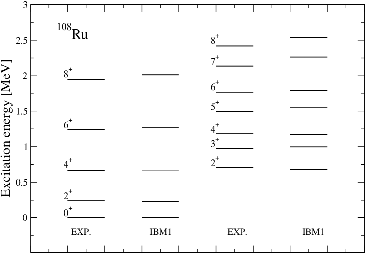
Figure 1: Experimental and calculated level schemes for ¹⁰⁸Ru.

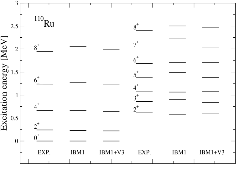
Figure 2: Experimental and calculated level schemes for ¹¹⁰Ru.

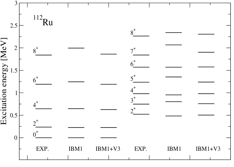
Figure 3: Experimental and calculated level schemes for ¹¹²Ru.

The comparison of the experimental levels with those calculated with the standard IBM-1 is presented in figs. 1, 2 and 3. For the ground-state bands only the levels up to spin $8^{+}$ were considered in the calculations since above this spin value the yrast bands exhibit a backbend in all nuclei. Also in the quasi-$\gamma$ bands, only levels up to spin $8^{+}$ were included in the fit. The full set of parameters of the Hamiltonian (3) obtained from the fit to the experimental data is given in table 1.

Table 1: IBM-1 parameters used in the present calculations with the standard Hamiltonian eq. (3). All parameters are given in units of MeV, except $\chi$ and $N$ which are dimensionless.

	108Ru	110Ru	112Ru
$\epsilon$	$\phantom{-}0.804\phantom{0}$	$\phantom{-}0.713\phantom{0}$	$\phantom{-}0.509\phantom{0}$
$\chi$	$-0.128\phantom{0}$	$-0.077\phantom{0}$	$-0.060\phantom{0}$
$\kappa$	$-0.0485$	$-0.0466$	$-0.0439$
$\lambda$	$\phantom{-}0.014\phantom{0}$	$\phantom{-}0.015\phantom{0}$	$\phantom{-}0.016\phantom{0}$
$\beta$	$-0.106\phantom{0}$	$-0.091\phantom{0}$	$-0.089\phantom{0}$
$N$	10	11	10

In the calculations all five parameters were allowed to vary. They were found to change smoothly when going from ¹⁰⁸Ru to ¹¹²Ru, indicating a slight change in structure when the boson number is varied.

A good agreement between the experimental and calculated energy levels of the ground-state band is obtained in all nuclei. The quasi-$\gamma$ band is well reproduced by the standard IBM-1 only in ¹⁰⁸Ru, whereas the much weaker staggering observed in ^110,112Ru is clearly overestimated by the model (see figs. 1, 2 and 3). The calculated odd-even staggering is characteristic of the SO(6) limit, whereas the staggering observed in ^110,112Ru is nearer to the RTRM pattern, as discussed in the previous section.

The accuracy of the fit can be easily seen from the plot of the signature splitting between the even- and odd-spin members of the band. The signature splitting functions $S(I)$ for the experimental and calculated levels in ^108,110,112Ru are represented in fig. 4 where $S(I)$ is given by [41]:

$$S(I)=\frac{E(I)-E(I-1)}{E(I)-E(I-2)}\cdot\frac{I(I+1)-(I-1)(I-2)}{I(I+1)-I(I-1)}-1.$$ (10)

The $S(I)$ function vanishes in the case of an axially symmetric rotor. As it can be seen in the lowest panel of fig. 4, the experimental signature splitting in ¹⁰⁸Ru can be well described by the calculations. In ^110,112Ru, however, the model fails to reproduce both the phase and magnitude of the experimental $S(I)$ (fig. 4, middle, top). Furthermore, the model predicts in both nuclei a slight decrease of the splitting with increasing spin, in disagreement with the empirical observations.

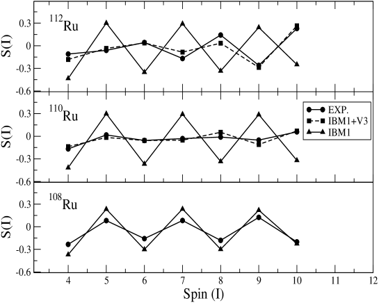
Figure 4: Experimental and calculated signature splitting for the quasi-$\gamma$ bands in ^108,110,112Ru.

3.2 Fit with the extended Hamiltonian

Since the odd-even staggering pattern of the quasi-$\gamma$ band in ^110,112Ru resembles that of a triaxially deformed rotor, it is natural to use the extended IBM-1 Hamiltonian, which may produce an energy surface with a triaxial minimum. Adding the $J=3$ cubic term to the standard IBM-1 Hamiltonian lowers the $I^{\pi}=3^{+},5^{+},7^{+},\dots$ states of the quasi-$\gamma$ band while the levels of the ground-state band and the even-spin members of the quasi-$\gamma$ band are only slightly affected. Therefore, the starting parameters for the fit with the extended version of the model were those obtained in the simplified version (see table 1), converted to the standard representation (6) (see table 2, column “IBM1”). The fitting procedure was carried out for different values of the strength $v_{3}$ of the cubic interaction until a reasonable agreement between the experimental and calculated energy spacings of the quasi-$\gamma$ band was obtained. Finally, all parameters were readjusted in order to obtain an overall agreement with the data.

Table 2: Parameters and rms deviations $\sigma$ given in units of MeV, except $\chi$ which is dimensionless.

	108Ru		110Ru			112Ru
	$N=10$		$N=11$			$N=10$
	IBM1		IBM1	IBM1+V3		IBM1	IBM1+V3
$\epsilon^{\prime}$	–.1.334		–.1.1680	–.1.2200		–.1.0350	–.1.0970
$a_{1}$	$-0.010$		$-0.0052$	$-0.0076$		$-0.0038$	$-0.0075$
$a_{2}$	$-0.049$		$-0.0466$	$-0.0466$		$-0.0439$	$-0.0439$
$a_{3}$	$-0.088$		$-0.076\phantom{0}$	$-0.065\phantom{0}$		$-0.074\phantom{0}$	$-0.058\phantom{0}$
$a_{4}$	$-0.206$		$-0.177\phantom{0}$	$-0.177\phantom{0}$		$-0.173\phantom{0}$	$-0.173\phantom{0}$
$\chi$	$-0.128$		$-0.077\phantom{0}$	$-0.127\phantom{0}$		$-0.060\phantom{0}$	$-0.100\phantom{0}$
$v_{3}$	—		—	$-0.030\phantom{0}$		—	$-0.035\phantom{0}$
$\sigma_{\rm g}$	$\phantom{-}0.062$		$\phantom{-}0.086\phantom{0}$	$\phantom{-}0.030\phantom{0}$		$\phantom{-}0.095\phantom{0}$	$\phantom{-}0.025\phantom{0}$
$\sigma_{\gamma}$	$\phantom{-}0.072$		$\phantom{-}0.098\phantom{0}$	$\phantom{-}0.034\phantom{0}$		$\phantom{-}0.102\phantom{0}$	$\phantom{-}0.030\phantom{0}$

The result of the fit with the extended IBM-1 Hamiltonian denoted IBM1+V3 is shown in fig. 2 for ¹¹⁰Ru and in fig. 3 for ¹¹²Ru and the parameters used in the calculations are given in table 2. The calculated levels for the quasi-$\gamma$ band in both nuclei now show a more regular energy spacing resulting in a much better agreement with the data. The addition of the cubic term accounts very well for the observed signature splitting (see fig. 4). These observations can be made quantitative by quoting the root-mean-square (rms) deviation between calculated and observed excitation energies. This is done in table 2 where rms deviations are given for the ground-state band up to $I^{\pi}=8^{+}$ (denoted as $\sigma_{\rm g}$) and for the quasi-$\gamma$-band up to $I^{\pi}=8^{+}$ (denoted as $\sigma_{\gamma}$). The quoted deviations prove that the addition of a cubic interaction leads to a substantial improvement of the energy fit for the quasi-$\gamma$ bands in ¹¹⁰Ru and ¹¹²Ru without destroying the agreement for the ground-state band.

A comparison between the experimental and calculated $B$(E2) ratios for some relevant interband and intraband transitions is given in table 3. The question may be asked whether all examined transitions have E2 multipolarity, as it has been assumed in most publications. The Evaluated Nuclear Structure Data File (ENSDF) [42] and the Nuclear Data Sheets contain a few values of the mixing ratio $\delta({\rm E2/M1})$ for ¹⁰⁸Ru. No $\delta$ values are known for ^110,112Ru. The relative $B$(E2) values for the $2_{2}\rightarrow 2_{1}$ and $3_{1}\rightarrow 2_{1}$ transitions in ¹⁰⁸Ru have been corrected for M1 contributions with the factors 0.95 and 0.9, respectively.

In the proton-neutron IBM-2, M1 transitions between symmetric states are forbidden. An M1 transition can occur only if there is an admixture of states containing antisymmetric bosons pairs ($F$-spin mixing) [43]. Such admixtures are usually weak in the excitation energy range considered in this work.

Table 3: Experimental and calculated E2 branching ratios for ^108,110,112Ru.

	108Ru			110Ru				112Ru
Ratio	EXP	IBM1		EXP	IBM1	IBM1+V3		EXP	IBM1	IBM1+V3
$\frac{2_{2}^{+}\rightarrow 2_{1}^{+}}{2_{2}^{+}\rightarrow 0_{1}^{+}}$	8.6(20)	7.1		14.9(2)	12.1	9.3		22.2(3)	10.6	16.7
$\frac{3_{1}^{+}\rightarrow 2_{2}^{+}}{3_{1}^{+}\rightarrow 2_{1}^{+}}$	15.9(14)	12.5		20.4(3)	14.3	14.3		21.7(4)	14.3	20.8
$\frac{4_{2}^{+}\rightarrow 2_{2}^{+}}{4_{2}^{+}\rightarrow 2_{1}^{+}}$	100(5)	100		100(6)	10	500		318(26)	166.7	1000
$\frac{4_{2}^{+}\rightarrow 2_{2}^{+}}{4_{2}^{+}\rightarrow 4_{1}^{+}}$	2.1(1)	2.4		1.1(1)	1.9	1.6		0.94(4)	1.85	1.3
$\frac{5_{1}^{+}\rightarrow 3_{1}^{+}}{5_{1}^{+}\rightarrow 4_{1}^{+}}$	10(1)	20		25(1)	27.8	30.3		37(2)	27.8	50
$\frac{4_{3}^{+}\rightarrow 3_{1}^{+}}{4_{3}^{+}\rightarrow 2_{2}^{+}}$				2.75(20)	19.75	0.62		0.66(3)	34.1	4.3

Most calculations are in good agreement with the experimental values. The small differences in the $B$(E2) ratios obtained with the two versions of the model are due to the slightly different values used for the $\chi$ parameter in the boson transition operator $\hat{T}({\rm E2})$ (see tables 1 and 2) and the inclusion of the cubic term in the extended IBM-1 Hamiltonian.

3.3 Effective $\gamma$

It is of interest to compare the calculation with the extended Hamiltonian with results of a global calculation of nuclear ground-state properties using the finite-range liquid-drop model (FRLDM) in which deviations from axial symmetry were allowed [44]. One of the regions in which nuclear ground states display triaxial deformation comprises the heavy Ru isotopes. In particular, the potential energy surface of ¹⁰⁸Ru has a shallow minimum at $\gamma\approx 21^{\circ}$. This energy surface can be described as being $\gamma$ soft.

Potentials obtained in the standard IBM-1 are $\gamma$ unstable for $\chi=0$ in the quadrupole operator $\hat{Q}^{\chi}$. For small, negative values of $\chi$ and an attractive quadrupole interaction $\hat{Q}^{\chi}\cdot\hat{Q}^{\chi}$ a shallow minimum develops for prolate deformation ($\gamma=0^{\circ}$). This minimum shifts towards $\gamma=30^{\circ}$ if a cubic interaction $v_{3}$ is added to the Hamiltonian. A more quantitative analysis can be made by calculating the quadratic and cubic invariants and relating them to the shape variables $\beta$ and $\gamma$ according to

$$\langle[\hat{Q}^{\chi}\times\hat{Q}^{\chi}]^{(0)}_{0}\rangle=\sqrt{\frac{1}{5}}\beta^{2},\qquad\langle[\hat{Q}^{\chi}\times\hat{Q}^{\chi}\times\hat{Q}^{\chi}]^{(0)}_{0}\rangle=-\sqrt{\frac{2}{35}}\beta^{3}\cos 3\gamma,$$ (11)

where $\langle\cdot\rangle$ denotes the expectation value for a particular state. A value for $\gamma$ can thus be deduced from the appropriate combination of the two invariants [45]. The deduced value can be considered as effective triaxiality, denoted by $\gamma_{\rm eff}$, as introduced by Yamazaki [46]. Results obtained in this way for ¹¹⁰Ru are shown in fig. 5. (Similar results are obtained for the two other isotopes.)

Figure 5: Effective values of $\gamma_{\rm eff}$ for states belonging to the ground (circles) and gamma (squares) bands in ¹¹⁰Ru. The full (dashed) lines join the values of $\gamma_{\rm eff}$ obtained in the standard (extended) IBM-1 calculation.

The values of $\gamma_{\rm eff}$ are fairly constant in the ground-state band (except for a slightly higher value in the ground state) and consistent with the results of the FRDLM for ¹⁰⁸Ru. Also, $\gamma_{\rm gsb}$ is found to be very close in the standard and the extended IBM-1. There is, however, a significant difference between the two calculations for the values of $\gamma_{\rm eff}$ for $\gamma$-band states with the pronounced even-odd staggering effect in the standard IBM-1 largely disappearing in the extended IBM-1. The differences between the two calculations are mainly due to the different choice for $\chi$ (see table 2) and the inclusion or not of a cubic interaction.

3.4 The 0${}^{+}_{2}$ state

Excited states at 976 and 1137 keV decaying to the $2^{+}_{1}$ level were observed in previous works in ^108,110Ru,  [8, 11]. Spin and parity $0^{+}$ were assigned to these states based on angular correlations measurements and the observed decay pattern. The recent work of Zhu et al. [7] confirms only the existence of a $0^{+}$ level at 975 keV in ¹⁰⁸Ru. States with $I^{\pi}=0^{+}$ located around 980 keV were also observed in the lighter ^104,106Ru isotopes. Stachel et al. suggested that these state might be based on intruder configurations [8, 9]. This configuration is produced by a proton(hole) pair excitation accross the shell closure at Z=50.

Zamfir [47] has studied this phenomenon in ¹⁰²Pd. A rather peculiar behaviour of the $0^{+}_{2}$ state, which cannot be explained by either IBM or E(5), has been ascribed to its intruder origin. At the same time, the authors caution against extrapolating this feature to heavier Pd isotopes. However, Lhersonneau and Wang [48, 49] investigated ^110,112,116Pd and observed typical intruder $0^{+}$ and $2^{+}$ states, with an energy minimum at ¹¹⁰Pd. It is not yet clear whether the same mechanism is working also in heavy Ru isotopes with $Z=44$. In order to answer this question better experimental information on the excited $0^{+}$ states in Ru is needed.

However, it is interesting to note that in ¹⁰²Ru, the $3^{+}_{1}$ state is located at 1522 keV and that with increasing neutron number the excitation energy of this state decreases, reaching 975 keV in ¹⁰⁸Ru. The energies of $0^{+}_{2}$ states, however, remain around 970 keV for the ^102-108Ru nuclei. In fact, this is the expected behaviour of the collective $0^{+}_{2}$ states for the U(5) to SO(6) transition in IBM-1. In the U(5) limit, the 0${}^{+}_{2}$ and 3${}^{+}_{1}$ states have $n_{d}=2$ and 3, respectively, whereas in the SO(6) limit both states belong to the multiplet with $\tau$=3. The calculation with the standard version of the IBM-1 Hamiltonian and the set of parameters given in table 1 predicts the 0${}^{+}_{2}$ state in ^108,110Ru with $(\tau,\nu_{\Delta})=(3,1)$ in the SO(6) limit at an energy of 896 and 763 keV, respectively, whereas the calculation for ¹¹⁰Ru with the extended IBM-1 Hamiltonian predicts this state at 1002 keV. The existence of $0^{+}$ states belonging to the $\sigma=N-2$ irrep of SO(6) cannot be a priori excluded. In any case, the observed $0^{+}_{2}$ state in ¹¹⁰Ru does not fit well into the systematics.

3.5 The band based on the $4^{+}_{3}$ state

An $I=4^{+}$ level located around 1.5 MeV excitation energy and the band-like structure based on it was identified in both ¹¹⁰Ru and ¹¹²Ru [7]. This band was observed up to spin 6⁺ in ¹¹⁰Ru and 9⁺ in ¹¹²Ru and it was found to exhibit a rather regular energy spacing between the even and odd spin members. In the SO(6) limit of the standard IBM-1 such states have $\tau\geq 4$, $\nu_{\Delta}=0$ and $\sigma=\sigma_{\rm max}$. The results of the fits are presented in fig. 6. The standard IBM-1 Hamiltonian fails to reproduce the observed weak staggering, whereas the addition of the cubic term improves the quality of the agreement. However, both versions of the model predict the $I=4^{+}$ bandhead $\sim 500$ keV lower in energy than experimentally observed. The standard version of the model clearly overestimates the ratio $B(E2;4^{+}_{3}\rightarrow 3^{+}_{1})/B(E2;4^{+}_{3}\rightarrow 2^{+}_{2})$ since in the SO(6) limit of IBM-1 such transitions have $\Delta\tau$=1 and $\Delta\tau$=2, respectively. The extended IBM-1 predicts a much lower branching ratio in both nuclei, thus giving a slightly better agreement with the experimental observations (see table 3).

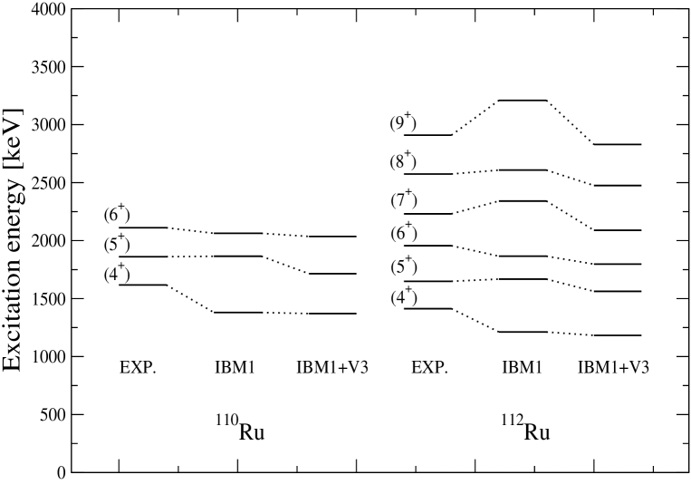
Figure 6: Experimental and calculated levels for the $K=4$ band in ^110,112Ru.

In the rotational model such a $4^{+}$ state is a candidate for a $\gamma$-$\gamma$ vibrational state, generated by a double $\gamma$-phonon excitation [15]. An equivalent interpretation can be formulated in the IBM by means of the quadrupole “phonon” excitation scheme [50]. In this case the quadrupole operator of eq. (4) plays a role similar to that of a phonon. In this scheme excited states can be generated by the multiple action of $\hat{Q}$ on the ground state. For instance,

$$|2^{+}_{1}\rangle=A\hat{Q}|0^{+}_{1}\rangle,\qquad|2^{+}_{2}\rangle=B[\hat{Q}\times\hat{Q}]^{(2)}|0^{+}_{1}\rangle,$$ (12)

and so on; $A$ and $B$ are normalization constants. If we generate the $4^{+}_{3}$ state in this way, we obtain in U(5) and SO(6) that

$$|4^{+}_{3}\rangle=\left(a[[\hat{Q}\times\hat{Q}]^{(2)}\times[\hat{Q}\times\hat{Q}]^{(2)}]^{(4)}+b[\hat{Q}\times\hat{Q}]^{(4)}\right)|0^{+}_{1}\rangle.$$ (13)

It has been shown [51] that $b\ll a$ so that, to a good approximation, the $4^{+}_{3}$ state is a four $Q$-phonon state. It can be symbolically represented as $[|2^{+}_{2}\rangle\otimes|2^{+}_{2}\rangle]^{(4)}$, where the two states are coupled to $L=4$. This is equivalent to what is usually called a double-$\gamma$ excitation. As a general remark, the nature of the $4_{3}^{+}$ states is not yet completely clear.

3.6 IBM-1 versus RTRM

The collective structure of ^{104,106,108,110,112}Ru was also previously discussed [3, 8, 10, 12] in the framework of the Rigid Triaxial Rotor Model (RTRM) [52]. It has been recognized that in these nuclei the $\gamma$ dependence of the potential is intermediate between the two limiting cases of a $\gamma$ unstable and a $\gamma$ rigid rotor [3, 8].

In ^108,110,112Ru, the experimental E2 branching ratios were found to be in overall agreement with those predicted by the RTRM calculations by using the $\gamma$-values 22.5^∘, 24.2^∘ and 26.4^∘, respectively, as deduced from the experimental $E_{2^{+}_{2}}/E_{2^{+}_{1}}$ energy ratio [3].

Figure 7 shows the comparison between the experimental B(E2) ratios divided by the ratios calculated with the IBM1 Hamiltonian (top), and RTRM model using the $\gamma$ values from [3] (bottom). In all cases, the experimental E2 branching ratios are rather well described by the models. However, an RTRM calculation of the odd-even staggering in the quasi-$\gamma$ band with the values of the triaxiality parameter $\gamma$ from [3], leads to a clear disagreement with experiment, as seen in figure 8. This should be compared with the fits shown in fig. 4.

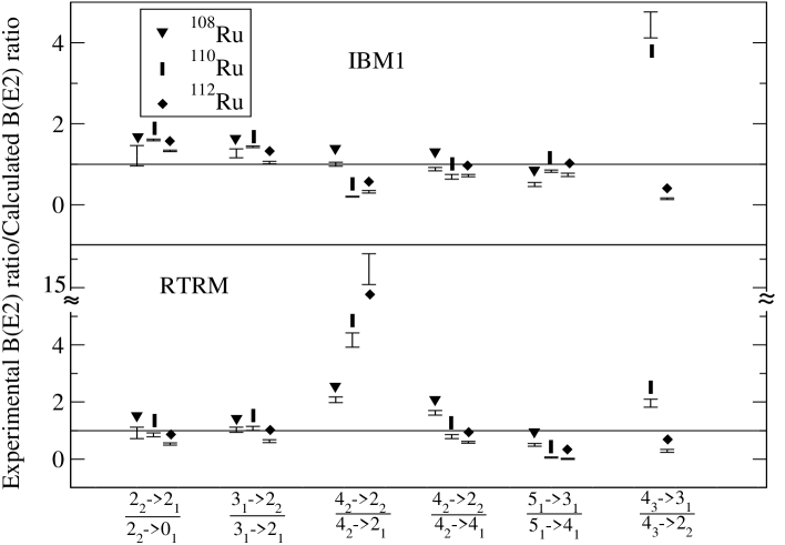
Figure 7: Experimental B(E2) ratios divided by the theoretical ratios calculated with the standard (¹⁰⁸Ru) and extended (^110,112Ru) IBM-1 Hamiltonian (top) and RTR model (bottom) with the $\gamma$-values given in ref. [3]. Please note the slight difference in the scales of the Y-axis for the two plots.

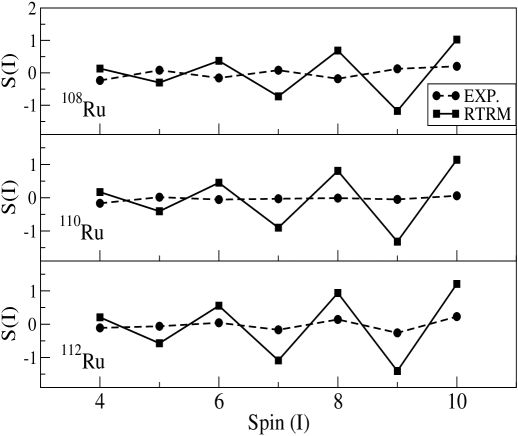
Figure 8: Comparison between the experimental and calculated signature splitting for the quasi-$\gamma$ bands in ^108,110,112Ru.

The difficulty of correctly describing at the same time excitation energies and E2 branching ratios is presumably the main problem of the RTRM [3, 53]. The authors of [53] assume that the use of moments of inertia based on the irrotational flow hypothesis is at the origin of the problem.

Contrary to the RTRM, the IBM, especially in the extended version with 3-body terms in the Hamiltonian, is able to describe most of the experimental data in the investigated nuclei (see figs. 2,3,4,6 and table 3).

Recently triaxiality has been studied in a more general geometrical context, by explicitly introducing a $\gamma$ soft potential  [54, 55].

3.7 Band structure

A sequence of states characterized by large values of $B$(E2) for transitions inside the sequence and connected by transitions with smaller $B$(E2)’s to other sequences (inter-band transitions) is usually called a band. Another characteristic of a collective band is the existence of a corresponding intrinsic state, i.e. of a state defined in the intrinsic coordinate frame (see [15]).

The concept of collective band has become so familiar that level schemes are usually drawn in such a way as to display the band structure. The question arises whether the collective excited states of a nucleus can always be classified into one-dimensional bands inter-connected by weak E2 transitions. This simple pattern cannot be seen in the investigated heavy Ru nuclides. In a nucleus with clear band structure, the ratio $B(E2;4_{2}\rightarrow 4_{1})/B(E2;4_{2}\rightarrow 2_{2})$ must be quite small. In ¹⁰⁸Ru this ratio has the value 0.69. Both transitions in numerator and denominator have $\Delta\tau=-1$. The ratio $B(E2;2_{2}\rightarrow 2_{1})/B(E2;2_{2}\rightarrow 0_{1})=15.6$ in the same nucleus. In this case, the upper transition has $\Delta\tau=-1$, while the lower one has $\Delta\tau=-2$ which is $\tau$-forbidden both in SO(6) and in U(5) with $\chi=0$. If the Alaga rule is applied, the ratio is 1.14.

What does the IBM-1 predict? In the SO(6) limit there are transitions with a large $B$(E2) value between the band based upon the $2_{2}$ state and the gb. Such bands have been called by Sakai [56] “quasi-$\gamma$ bands”. The strong E2 transitions in the investigated nuclei are those with $\Delta\tau=\pm 1$.

It has been shown by Leviatan [57] that in the SO(6) limit of the IBM, all states belonging to the lowest irrep of SO(6), i.e. the states with $\sigma=N$, can be projected out of a single intrinsic state.

4 Conclusion

Excitation energies and E2 ratios in ^108,110,112Ru have been calculated with the IBM-1. First, a standard IBM-1 approach with only one- and two-body terms has been used. A good fit was obtained for ¹⁰⁸Ru. However, the odd-even staggering in the quasi-$\gamma$ band of ^110,112Ru was not correctly described by the model. The experimental staggering was rather close to the pattern predicted by the triaxial rotor model.

Subsequently, an extended Hamiltonian which contains three-body terms has been used. It is known that this type of Hamiltonian can generate a triaxial minimum of the total energy surface. With this Hamiltonian the odd-even staggering in the quasi-$\gamma$ band was correctly reproduced while the excitation energies and the $B$(E2) ratios of even-spin states were hardly affected. In addition, effective values of $\gamma$ have been calculated.

It has been observed, in agreement with previous investigations, that these nuclei are intermediate between the U(5) and the SO(6) limits of the IBM. There is no equivalent interpretation in the rigid triaxial rotor model. However, none of these nuclides corresponds exactly to either the U(5) or the SO(6) symmetry. The $d$-boson seniority $\tau$ is an approximately good quantum number, which allows one to classify the excited states and to understand the $B$(E2) ratios.

The results obtained with the Interacting Boson Model have been compared to those of the Rigid Triaxial Rotor Model. While the $B$(E2) ratios have been equally well described by both models, the odd-even staggering in the quasi-$\gamma$ bands has been correctly reproduced only by the IBM.

The band structure of ^108,110,112Ru has been discussed. Contrary to the situation in the axially deformed nuclei, the $B$(E2) ratios show that there are interband transitions with E2 strengths of the same order of magnitude as that of intraband transitions.

5 Acknowledgements

The authors would like to thank Dr. B. Saha, S. Heinze, Prof. P. Möller, Prof. V. Werner and Prof. J. Wood for interesting discussions and communication of unpublished work. This work has been supported by the Deutsche Forschungsgemeinschaft under grant JO391/3-2, IAP Research Program no. P6/23 and FWO-Vlaanderen (Belgium).

References

- [1] J. H. Hamilton et al., Prog. Part. Nucl. Phys. 35 (1995) 635.
- [2] J. H. Hamilton et al., Nucl. Phys. A 734 (2004) 257.
- [3] J.A. Shannon et al., Phys. Lett. B 336 (1994) 136.
- [4] Q. H. Lu et al., Phys. Rev. C 52 (1995) 1348.
- [5] X. L. Che et al., China Phys. Lett. 21 (2003) 1904.
- [6] H. Hua et al., China Phys. Lett. 20 (2003) 350.
- [7] S. J. Zhu et al., preprint, to be published.
- [8] J. Stachel et al., Z. Phys. A 316 (1984) 105.
- [9] J. Stachel et al., Nucl. Phys. A 383 (1982) 429.
- [10] J. Äystö et al., Nucl. Phys. A 515 (1990) 365.
- [11] J. C. Wang et al., Phys. Rev. C 61 (2000) 044308.
- [12] J. Srebrny et al., Nucl. Phys. A 766 (2006) 25.
- [13] J. Stachel, P. Van Isacker and K. Heyde, Phys. Rev. C 25 (1982) 650.
- [14] F. Iachello and A. Arima, The Interacting Boson Model, Cambridge University Press, Cambridge, 1987.
- [15] A. Bohr and B. R. Mottelson, Nuclear Structure. II Nuclear Deformations, Benjamin, Reading, Mass., 1975.
- [16] L. Wilets and M. Jean, Phys. Rev. 102 (1956) 788.
- [17] A. Giannatiempo, A. Nannini, P. Sona and D. Cutoiu, Phys. Rev. C 52 (1995) 2969.
- [18] J. L. Duarte et al., Phys. Rev. C 57 (1998) 1539.
- [19] A. Arima, T. Otsuka, F. Iachello and I. Talmi, Phys. Lett. B 66 (1977) 205.
- [20] F. Iachello, Phys. Rev. Lett. 53 (1984) 1427.
- [21] P. Van Isacker, K. Heyde, J. Jolie and A. Sevrin, Ann. Phys. (N.Y.) 171 (1986) 253.
- [22] A. Frank, C. E. Alonso and J. M. Arias, Phys. Rev. C 65 (2001) 014301.
- [23] J. N. Ginocchio and M. W. Kirson, Phys. Rev. Lett. 44 (1980) 1744.
- [24] A. E. L. Dieperink, O. Scholten and F. Iachello, Phys. Rev. Lett. 44 (1980) 1747.
- [25] F. Iachello, Phys. Rev. Lett. 85 (2000) 3580.
- [26] J. M. Eisenberg and W. Greiner, Nuclear Theory I, North-Holland, Amsterdam, 1987.
- [27] D. Troltenier et al., Z. Phys. A 338 (1991) 261.
- [28] D. Troltenier et al., Nucl. Phys. A 601 (1996) 56.
- [29] C. Y. Wu et al., Phys. Rev. C 73, (2006) 034312.
- [30] B. Saha, et al., Phys. Rev. C 70 (2004) 034313.
- [31] X.-W. Pan, T. Otsuka, J.-Q. Chen and A. Arima, Phys. Lett. B 287 (1992) 1.
- [32] R. F. Casten, Nuclear structure from a simple perspective, Oxford University Press, Oxford, 2000.
- [33] I. Talmi, Simple models of complex nuclei, Harwood, Chur, 1993.
- [34] O. Scholten, Program PHINT, NSCL, MSU, 1982 (unpublished).
- [35] B. Saha, Program Phinema, Ph.D. thesis, University of Koeln, 2004 (unpublished).
- [36] R. F. Casten, P. von Brentano, K. Heyde, P. Van Isacker and J. Jolie, Nucl. Phys. A 349 (1985) 289.
- [37] P. M. Gore et al., EPJA 25 s01 (2005) 471.
- [38] P. Van Isacker and J. Q. Chen, Phys. Rev. C 24 (1981) 684.
- [39] K. Heyde, P. Van Isacker, M. Waroquier and J. Moreau, Phys. Rev. C 29 (1984) 1420.
- [40] P. Van Isacker, Program ibm1, GANIL (unpublished).
- [41] N.V. Zamfir and R. F. Casten, Phys. Lett. B 260 (1991) 265.
- [42] National Nuclear Data Center, http://www.nndc.bnl.gov
- [43] T. Otsuka, in: Algebraic approaches to nuclear structure, ed. R. F. Casten (Harwood Academic, Langhorne, USA, 1993).
- [44] P. Möller et al., Phys. Rev. Lett. 97 (2006) 162502.
- [45] J. P. Elliott, J. A. Evans and P. Van Isacker, Phys. Rev. Lett. 57 (1986) 1124.
- [46] T. Yamazaki et al., J. Phys. Soc. Jap. 44 (1978) 1421.
- [47] N. V. Zamfir et al., Phys. Rev. C 65 (2002) 044325.
- [48] G. Lhersonneau et al., Phys. Rev. C 60 (1999) 014315.
- [49] Y. Wang et al., Phys. Rev. C 63 (2001) 024309.
- [50] G. Siems et al., Phys. Lett. B 320 (1994) 1.
- [51] R. V. Jolos, A. Gelberg and P. von Brentano, Phys. Rev. C 53 (1996) 168.
- [52] A. S. Davydov and G. F. Filippov, Nucl. Phys. 8 (1958) 237.
- [53] J. Wood et al., Phys. Rev. C 70 (2004) 024308
- [54] L. Fortunato, Phys. Rev. C 70 (2004) 011302.
- [55] L. Fortunato, S. De Baerdemacker and K. Heyde, Phys. Rev. C 74 (2006) 014310.
- [56] M. Sakai, At. Data Nucl. Data Tables 31 (1984) 399.
- [57] A. Leviatan, Ann. Phys. (N.Y.) 179 (1987) 201 and references therein.