Institute of Quantum Materials Science, 620107 Ekaterinburg, Russia
Institute for Molecules and Materials, Radboud University Nijmegen, 6525 ED Nijmegen, The Netherlands
Order-disorder transformations; statistical mechanics of model systems Magnetomechanical and magnetoelectric effects, magnetostriction Self-organized systems
Intrinsic nanoscale inhomogeneity in ordering systems due to elastic-mediated interactions
Abstract
Phase diagram and pattern formation in two-dimensional Ising model with coupling between order parameter and lattice vibrations is investigated by Monte-Carlo simulations. It is shown that if the coupling is strong enough (or phonons are soft enough) a short-range order exists in disordered phase for a broader temperature interval. Different types of this short-range order (stripe-like, checkboard-like, etc.) depending on the temperature and model parameters are investigated. With further increase of the coupling, a reconstruction of the ground state happens and new ordered phases appear at low enough temperatures.
pacs:
64.60.Cnpacs:
75.80.+qpacs:
05.65.+b1 Introduction
Traditional views assume that under the thermodynamic equilibrium conditions a system should either be homogeneous or consist of macroscopically large domains of homogeneous phases. It appears frequently, however, that equilibrium or very long-lived metastable states occur with a nanoscale or mesoscale heterogeneity (for a general review of these phenomena in various physical and chemical systems see, e.g., Refs.[1, 2, 3, 4]). It is commonly accepted now that the formation of the mesoscale heterogeneity is a result of frustrations in the system which can result from either geometric factors [4, 5, 6, 7] or competing interactions, the long-ranged forces such as Coulomb or dipole-dipole interactions being of primary importance [4, 8, 9, 10, 11, 12, 13, 14].
“Heterophase” fluctuations in metallic alloys [15] provide us interesting examples of intrinsic nanoscale inhomogeneities. In such cases, a system behaves like an ensemble of nanosize particles of one phase embedded into the matrix, e.g., so-called athermic -phase in bcc host which is observed in some Ti- and Zr-based alloys [16], as well as in Cr1-xAlx [17]. This peculiar structural state leads to strong anomalies of electronic properties [18] and ultrasound attenuation [19]. The “athermic -phase” is a term to describe rather some short-range order in atomic positions than real phase since it never exists in the bulk (atomic positions in this “phase” are intermediate between bcc structure and true -phase existing in Ti and Zr under pressure). It would be not surprising to observe strong short-range order in the close vicinity of a second-order phase transition. On the contrary, these heterophase fluctuations sometimes arise in a broad temperature and concentration domain. Nature of this state is still unknown (see discussions in Refs.[7, 15]).
A well-pronounced short-range order or nanoscale inhomogeneity in a broad temperature interval are often observed in magnetic alloys with a strong coupling between magnetism and lattice (or chemical composition), such as Cu-Mn alloys [20, 21] or Fe-Ni Invar alloys [22, 23]. As mentioned above it is a tendency now to connect intrinsic inhomogeneities in various systems with long-range interactions. One may expect therefore that a long-range character of elastic deformations is solids could be relevant for the problem under discussion.
To clarify a role of elastic-mediated interactions in possible pattern formation we have investigated the simplest model of Ising order parameter coupled with phonons at the square lattice. Basing on the results of Monte Carlo simulations for this model we show that, indeed, this coupling can result in a formation of various nanosize-scale structures.
2 Model and computational details
The two-dimensional Ising model [24, 25] is a prototype, exactly solvable model of order-disorder phase transitions in magnetic systems, ordering alloys, etc. To be specific we will use further terms “magnetic” and “spins” to describe the ordering phenomena under consideration. To describe the effects of magnetoelastic (spin-lattice) interactions, we proceed with the Hamiltonian
| (1) |
where if are the nearest neighbors and is equal to zero, otherwise, are atomic displacement vectors and spin variables . The spin–lattice coupling is taken into account via coordinate dependence of the exchange parameters , being square lattice vectors. Assuming that the displacements are small the exchange parameters can be written in the linear approximation
| (2) |
where is the unit vector in direction of .
Substituting Eq.(2) into Eq.(1) and assuming periodic boundary conditions we obtain
| (3) |
where . The dependence of the exchange parameters on interatomic distances results in the last term in right-hand-side of Eq.(3)
| (4) |
describing forces acting on atoms due to spin redistribution. These forces initiate the displacements of atoms into new equilibrium positions determined by the expression
| (5) |
where , is the static lattice Green’s function determined by the equation
| (6) |
Replacing the variables one can represent the partition function as
| (7) |
where the effective spin Hamiltonian
| (8) |
and is the inverse temperature.
Due to harmonic approximation for the potential energy of atomic displacements and linear approximation for the magnetoelastic coupling the phonon and spin subsystems turn out to be totally separated after the change of variables. The statistical properties of the system is completely determined by the Hamiltonian which depends on spin variables only. The last term in the right-hand-side of Eq.(8) reads
| (9) |
and describes indirect long-range spin-spin interactions via lattice distortions.
To investigate equilibrium properties of the spin system with the Hamiltonian (8) we have carried out the Monte Carlo simulations for the square lattice with 100 100 sites and periodic boundary conditions, using a standard Metropolis algorithm [26]. To provide the Gibbs distribution we have performed up to 104 flips for each lattice spin.
We are interested in the two-dimensional spin system embedded into three-dimensional elastic medium. For two-dimensional continuum the Green’s function is pathological, with logarithmic growth at large distances. Instead, we use the expression
| (10) |
valid in the framework of quasi-continuum approach [27] with isotropic Debye model for the phonon spectra. Here is the integral sine function [28], is the lattice parameter, is the shear modulus which can be expressed [27] in terms of the force constants . The Green’s function (10) has asymptotic behavior at large distances. To speed up computations, we use its truncation by multiplying expression (10) by . The length and phonon-induced interaction cut-off radius were chosen at 5th and 13th neighbors, respectively; these values ensure the convergency and stability of computational results.
For the bare exchange parameters the nearest-neighbor (nn) interactions have been taken into account. The choice of nn parameter determines the energy units.
| a | b | c | d |
|---|---|---|---|
 |
 |
 |
 |
| a | b | c | d |
|---|---|---|---|
 |
 |
 |
 |
3 Results of the Monte Carlo simulations
In the square-lattice Ising model with nn interactions the phase transition takes place at . One can see (Fig. 1) that the true ground state is reached for approximately 104 spin flips per spin whereas for shorter Monte Carlo runs metastable configurations such as domain walls appear. Further we will use by default this number of flips. Probably it is not enough for a close vicinity of due to critical slowing down but we will not discuss this region.
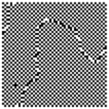
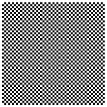
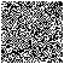
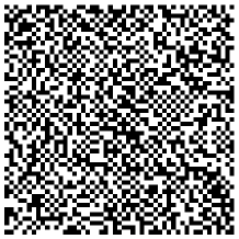
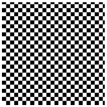
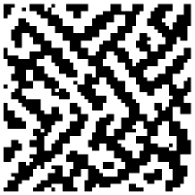
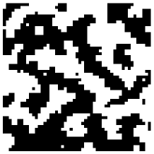
The effects of long-range interactions due to magnetoelastic coupling are crucially dependent on dimensionless coupling constant . Nontrivial patterns in a broad enough temperature interval both below and above arise at ; typical spin configurations are shown in Fig. 2. In this case we have found a long-range or short-range order of checkboard or stripe types with staggered spin-up and spin-down regions. These patterns appear when MC simulations start from both random and from regular initial spin distribution and, therefore, are not metastable but, rather, equilibrium states. Pictures of the long-range order are quite similar for the case of FM () and AFM () Ising model.
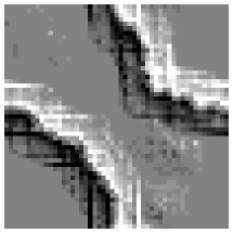
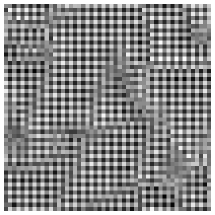
Since these new types of ordering result from the coupling between magnetic and elastic subsystems it is naturally to expect its manifestations also in the distribution of the displacement field (Fig. 3). For weak magnetoelastic coupling the lattice distortions are created by domain boundaries in metastable configurations and spread over large distances due to a slow decay of . Fig. 3a shows the corresponding distribution calculated by the perturbation theory in the lowest order in . Spin patterns at large are inevitably related with the lattice distortion chessboard patterns visible in Fig. 3b. Contrary to previous case, deformations are mutually cancelled at large spatial scale.
| a | b |
|---|---|
 |
 |
| FM | AFM | |||
|---|---|---|---|---|
| -4 | -3 | 4 | 3 | |
| FM | -4.0 | -4.0 | 4.0 | 4.0 |
| AFM | 4.0 | 4.0 | -4.0 | -4.0 |
| R | -1.8 | -1.0 | -1.8 | -1.0 |
| c2x2 | -5.3 | -3.0 | -5.3 | -3.0 |
| c3x3 | -4.2 | -2.9 | -1.6 | -0.3 |
| c2x3 | -4.8 | -3.0 | -3.5 | -1.7 |
| s2x1 | -4.7 | -2.6 | -4.7 | -2.6 |
| s3x1 | -4.2 | -2.9 | -1.5 | -0.3 |


To understand character of new types of ordering let us consider energies of different local spin configurations (Fig. 4). For ferromagnetic ordering (Fig. 4a) the force (4) and therefore the magnetoelastic contribution to the total energy vanishes. On the other hand, the configuration Fig. 4b corresponds to the largest local value of and, thus, to the maximal magnetoelastic energy gain. This configuration is a minimal structural block of stripe and checkboard structures. Direct total energy calculations for various spin configurations (see the Table) demonstrate that at simple FM or AFM structure become energetically unfavorable and the new ordered ground state occurs. In this case the checkboard ordering is preferable and the stripe structure has slightly higher energy.
With the temperature increase, the long-range order is destroyed. We estimate critical temperatures of these transitions calculating the -dependence of pair correlation functions of the corresponding order parameters. The results are presented in Figure 5. With the growth of the temperature of transition from FM (AFM) and paramagnetic phase decreases. This is not surprizing since the magnetoelastic coupling destabilizes these spin states. With further increase of there is a transition between check-board (or stripe) phase and the paramagnetic state, the transition temperature growing with .

Figure 6 shows the evolution of the spin correlation functions for (that is, at the transition between regions 1 and 3 at the phase diagram 5) with the temperature increase. One can see that the magnetoelastic coupling leads to stronger short-range order above (c.f. curves 2 and 2’, 3 and 3’, respectively), which survives up to a relatively higher temperature, in comparison with the original Ising model. In particular, the short-range order for and (curve 5) is stronger than for and (curve 4).
The short-range order in the region 3 near the triple point tends to formation of stripe-like structures (Fig. 2b,c), although this configuration is not the most energetically preferable. The appearance of this structure is connected with its higher entropy in comparison with the checkboard structure.
4 Discussion and conclusions
Our computational results are summarized schematically in the phase diagram shown in Fig. 5. For small enough coupling constant the behavior of the system is qualitatively similar to that of the standard Ising model. In this case the main effect of the magnetoelastic coupling is suppression of due to destabilization of FM or AFM states (Fig. 6). Usually this happens if is strongly suppressed by soft fluctuations, such as in quasi-two-dimensional Heisenberg magnets [29] or frustrated three-dimensional Heisenberg magnets with competing interaction [30]. In those cases is much smaller than a typical energy of nearest-neighbor interaction whereas the short-range order in a broad temperature interval survives up to the temperatures of order of . We illustrate here an alternative mechanism of occurrence of the short-range order due to coupling with a second subsystem providing long-range effective interactions.
Thus, in this regime the magnetoelastic interactions are favourable for the short-range order in paramagnetic phase but do not result yet in the nontrivial pattern formation. The latter happens at where exotic spin configurations (checkboard or stripe states) become favourable. Especially, near the triple point at the phase diagram (Fig. 5) there are many different states with approximately the same free energy and therefore a formation of complicated inhomogeneous states could be expected. At further temperature increase we reach a conventional paramagnetic (random) state without short-range order. This scenario reminds the behavior observed at the “melting” of stripe domains in magnetic films [11], our “pattern” regime being similar to “tetragonal phase” in the latter case. The main formal difference between these two problems is two-spin character of long-range dipole-dipole interactions versus four-spin character of long-range phonon-mediated interaction considered here.
Despite a simplicity of our model, it demonstrates a rather general feature which we believe can be relevant for discussions of real systems demonstrating a strong short-range order above in a broad temperature interval. The effect arises at large enough coupling constant which means either unusually strong interaction between the subsystems (large ) or soft phonons (small shear modulus). At least, in some case, such as Cu-Mn alloys the shear modulus tends to zero at some critical composition or temperature [21] so can be, in principle, arbitrarily large. It would be interesting to analyse the problem of heterophase fluctuations in alloys mentioned in the Introduction from this point of view.
Acknowledgements. The work was supported by the Netherlands Organization for Scientific Research (NWO project 047.016.005) and by the Stichting Fundamenteel Onderzoek der Materie (FOM).
References
- [1] Seul M. and Andelman D., Science 267 (1995) 476.
- [2] Supramolecular Chemistry and Self-Assemlby. Special Issue: Science, 295 (2002) 2400-2421.
- [3] Dagotto E., Science, 309, (2005) 257.
- [4] Tarjus G., Kivelson S. A., Nussinov Z., and Viot P., J. Phys.: Condens. Matter, 17 (2005) R1143.
- [5] Kleman M., Adv. Phys., 38 (1989) 605.
- [6] Nelson D. R., Defects and Geometry in Condensed Matter Physics (Cambridge Univ. Press, Cambridge) 2002.
- [7] Gornostyrev Yu. N., Katsnelson M. I., and Trefilov A. V., J. Phys.: Condens. Matter, 9 (1997) 7837.
- [8] Emery V. J. and Kivelson S. A., Physica C, 209(1993) 597.
- [9] Kivelson D., Kivelson S. A., Zhao X., Nussinov Z., and Tarjus G., Physica A 219 (1995) 27.
- [10] Nussinov Z., Rudnick J., Kivelson S. A., and Chayes L. N., Phys. Rev. Lett., 83 (1999) 472.
- [11] De’Bell K., MacIsaac A. B., and Whitehead J. P., Rev. Mod. Phys., 72 (2000) 225.
- [12] Schmalian J. and Wolynes P. G., Phys. Rev. Lett., 85 (2000) 836.
- [13] Jagla E. A., Phys. Rev. E, 70 (2004) 046204.
- [14] Prudkovskii P. A., Rubtsov A. N., and Katsnelson M. I., Europhys. Lett., 73 (2006) 104.
- [15] Krivoglaz M. A., Zh. Eksper. Teor. Fiz., 84 (1983) 355 [Engl. transl.: Sov. Phys. JETP, 57 (1983) 205].
- [16] Collings E. W., The Physical Metallurgy of Titanium Alloys (American Society of Metals, Columbus OH) 1984.
- [17] Sudareva S. V., Rassokhin V. A., and Prekul A. F., Phys. Stat. Sol. (a) 76 (1983) 101.
- [18] Katsnelson M. I. and Trefilov A. V., Pis’ma ZhETF, 59(1994) 198 [Engl. transl.: JETP Lett., 59 (1994) 211 (1994)]; Pis’ma ZhETF 61 (1995) 920 [Engl. transl.: JETP Lett., 61 (1995) 941].
- [19] Gornostyrev Yu. N., Katsnelson M. I., and Trefilov A. V., Pis’ma ZhETF, 60 (1994) 213 [Engl. transl.: JETP Lett., 60 (1994) 221].
- [20] Vitaikin E. Z., Sakhno V. M., and Udovenko V. A., Dokladi AN SSSR, 246 (1979) 315.
- [21] Tsunoda Y., Orishi N., and Kunitomi N., J. Phys. Soc. Japan, 53 (1984) 359.
- [22] Menshikov A. Z., Physica B, 161 (1989) 1.
- [23] The Invar Effect: A Centennial Symposium, ed. by J. Wittenauer (TMS, Warrendale PA) 1997.
- [24] Ziman J. M., Models of Disorder (Cambridge Univ. Press, Cambridge) 1979.
- [25] Feynman R. P., Statistical Mechanics (Benjamin, Reading MA) 1972.
- [26] Landau D. P. and Binder K., A Guide to Monte Carlo Simulations in Statistical Physics (Cambridge Univ. Press, Cambridge) 2005.
- [27] Kunin I. A., Elastic Media with Microstructure II (Springer-Verlag, New York) 1982.
- [28] Abramowitz M. and Stegun I. A., Handbook of Mathematical Functions (Dover, New York) 1964.
- [29] Irkhin V. Yu., Katanin A. A., and Katsnelson M. I., Phys. Rev. B, 60 (1999) 1082.
- [30] Irkhin V. Yu., Katanin A. A., and Katsnelson M. I., J. Phys.: Condens. Matter, 4 (1992) 5227.