Spatiotemporal structure of Lyapunov vectors in chaotic coupled-map lattices

Abstract

The spatiotemporal dynamics of Lyapunov vectors (LVs) in spatially extended chaotic systems is studied by means of coupled-map lattices. We determine intrinsic length scales and spatiotemporal correlations of LVs corresponding to the leading unstable directions by translating the problem to the language of scale-invariant growing surfaces. We find that the so-called ‘characteristic’ LVs exhibit spatial localization, strong clustering around given spatiotemporal loci, and remarkable dynamic scaling properties of the corresponding surfaces. In contrast, the commonly used backward LVs (obtained through Gram-Schmidt orthogonalization) spread all over the system and do not exhibit dynamic scaling due to artifacts in the dynamical correlations by construction.

Lyapunov exponents (LEs) measure the exponential separation (or convergence) of nearby trajectories and provide the most common tool to characterize spatiotemporal chaos (STC) eckmann ; Bohr ; Ott . Not only exponential separation rates but also spatial correlations are crucial to deal with predictability questions in extended systems primo07 . Basically, (almost) any initial infinitesimal perturbation evolves in time asymptotically aligning along the most unstable direction, i.e. the main Lyapunov vector (LV). In extended systems, the main LV is found to be localized in space at any given time. However, due to spatial homogeneity, all directions in tangent space are actually equivalent and the localization center keeps moving all over the system. This is known as ‘dynamic localization’ of the main LV pik94 ; pik98 .

In the last decade, there has been some progress in the study of STC with tools borrowed from nonequilibrium statistical physics. In particular, the evolution of perturbations in spatially extended chaotic systems has been shown to be described by multiplicative Langevin-type equations pik94 ; pik98 ; lopez ; sanchez . In many cases pik98 , the dynamics of perturbations can be expressed in terms of the prototypical stochastic surface growth equation of Kardar-Parisi-Zhang (KPZ), $\partial_{t}h=(\partial_{x}h)^{2}+\partial_{xx}h+\zeta$, where $\zeta$ is a white noise kpz .

In this Rapid Communication we study the spatiotemporal structure of STC encoded by the LVs. We show that a family of vectors —that we shall call characteristic LVs— carry important information about the real-space structure, localization properties and space-time correlations. These properties are disclosed only after a logarithmic transformation, so that each LV is mapped into a rough surface. Our results greatly strengthen the link between STC and certain nonequilibrium surface growth models. We also find that the most widely used orthogonal LVs —that appear in the standard Gram-Schmidt procedure to compute the LEs benettin80 ; wolf85 — lack many of these features due to the construction procedure and, therefore, have much less physical significance.

We illustrate our results by numerical simulations of coupled map lattices (CMLs), which are a prototype of spatially extended dynamical systems exhibiting chaos. The main advantage of CMLs, as compared with e.g., partial differential equations, is their lower computational cost. We consider an array of $L$ maps diffusively coupled to nearest-neighbors:

$$u_{i}(t+1)=\epsilon f(u_{i+1}(t))+\epsilon f(u_{i-1}(t))+(1-2\epsilon)f(u_{i}(t)),$$ (1)

where $\epsilon$ is the coupling parameter and $f$ a map with chaotic dynamics. Throughout this paper, we consider the logistic map $f(y)=4y(1-y)$ with periodic boundary conditions. We follow the standard convention and sort LEs in decreasing order $\lambda_{1}\geq\lambda_{2}\geq\cdots\geq\lambda_{L}$. The coupling parameter is chosen to be $\epsilon=0.1$, and the system is hyperchaotic with $\lambda_{n}>0$ for $n/L<0.795$.

Lyapunov vectors.- Given the initial state of the system ${\bm{u}(t=0)=[u_{1}(0),u_{2}(0),\cdots,u_{L}(0)]}$, any infinitesimally small change ${\bm{\delta u}}(t=0)$ in the initial condition evolves up to linear order (i.e. in tangent space) according to

$$\delta u_{i}(t+1)=\epsilon f^{\prime}(u_{i+1}(t))\delta u_{i+1}(t)+\epsilon f^{\prime}(u_{i-1}(t))\delta u_{i-1}(t)$$ (2)

$$+(1-2\epsilon)f^{\prime}(u_{i}(t))\delta u_{i}(t)\equiv\sum_{j=1}^{L}T_{ij}[{\bm{u}}(t)]\delta u_{j}(t)$$ ,

with $f^{\prime}$ being the derivative of $f(y)$ with respect to $y$ and $\mathrm{\mathbf{T}}[{\bm{u}}(t)]$ the $L\times L$ Jacobian matrix evaluated at ${\bm{u}}(t)$. The evolution of an infinitesimal perturbation $\bm{\delta u}(t_{1})$ is governed by the linear equation (tangent space): ${\bm{\delta u}}(t_{2})=\mathrm{\mathbf{M}}(t_{2},t_{1}){\bm{\delta u}}(t_{1})$. The linear operator $\mathrm{\mathbf{M}}$ is just the product of the Jacobian matrices evaluated along the system trajectory from $t_{1}$ to $t_{2}$, i.e. $\mathrm{\mathbf{M}}(t_{2},t_{1})\equiv\mathrm{\mathbf{T}}[{\bm{u}}(t_{2}-1)]\mathrm{\mathbf{T}}[{\bm{u}}(t_{2}-2)]\ldots\mathrm{\mathbf{T}}[{\bm{u}}(t_{1})]$.

According to Oseledec’s theorem oseledec (details can be found in eckmann ) there exists the limit operator ${\bm{\Phi}}_{\infty}(t_{2})=\lim_{t_{1}\to-\infty}[{\mathrm{\mathbf{M}}(t_{2},t_{1})}{\mathrm{\mathbf{M}}(t_{2},t_{1})}^{*}]^{\frac{1}{2(t_{2}-t_{1})}}$, such that the logarithms of the eigenvalues are the LEs $\lambda_{n}$, and the eigenvectors form an orthonormal basis $\{{\mathbf{e}_{n}(t)}\}$. This set of eigenvectors, so-called backward LVs legras96 , indicates the directions of growth of perturbations grown since the remote past. The backward LVs are precisely the orthonormal vectors obtained using the standard Gram-Schmidt orthogonalization method to compute the LEs ershov98 .

As we will show below a much more interesting set of vectors $\{{\mathbf{g}_{n}(t)}\}$ are the so-called characteristic LVs. These are free-evolving perturbations that grow with exponent $\lambda_{n}$ ($-\lambda_{n}$) when integrating to the far future (past): $\lim_{|t_{2}|\to\infty}(t_{2}-t_{1})^{-1}\ln||{\mathrm{\mathbf{M}}}(t_{2},t_{1})\mathbf{g}_{n}(t_{1})||=\lambda_{n}$. Characteristic LVs are independent of the scalar product and do not form an orthogonal basis, in contrast to backward LVs. Also, they exhibit remarkable physical properties as they reduce to the Floquet eigenvectors for a periodic orbit trevisan98 ; and for autonomous continuous-time systems the null LE is associated with a characteristic LV tangent to the trajectory. This contrasts with the counterintuitive arrangement of backward LVs. We want to emphasize that characteristic LVs evolve freely, whereas backward LVs (other than the first one) do not map into themselves under time evolution.

Recently, characteristic LVs are receiving growing attention legras96 ; trevisan98 ; wolfe_tellus07 ; ginelli07 . Unfortunately, these vectors are difficult to compute because information from both the remote past (via backward LVs), and the remote future (via forward LVs) is needed . We have computed the characteristic LVs from the intersection of embedded subspaces from backward and forward LVs as described in Refs. legras96 ; wolfe_tellus07 . The $n$th characteristic LV is a linear combination of the backward LVs from 1 to $n$, and viceversa; and in particular ${\mathbf{g}_{1}(t)}={\mathbf{e}_{1}(t)}$. Our computational resources allowed us to achieve the very reasonable system size of $L=1024$.

Figure 1: (Color online) (a,b) Snapshot of the profiles of LVs with $n=1,2$ for system (1) with $L=512$ (note that we are taking the absolute values and a logarithmic scale). (c,d) Space-time evolution of the maxima of LVs from the 1st to the 10th. The position of the maximum for the first LV is indicated with big $\bullet$ symbols. Other symbols correspond to LVs for $n=2,\ldots,10$.

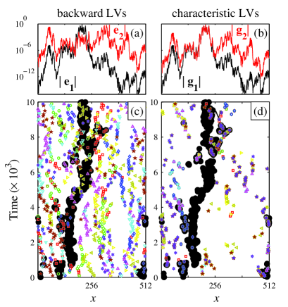
Localization of Lyapunov vectors.- Figure 1(a,b) shows the first and second LVs in logarithmic scale; the plots indicate strong localization. In Fig. 1(c,d) we plot the time evolution for the maxima of $|\mathbf{e}_{n}(t)|$ and $|\mathbf{g}_{n}(t)|$ for $n=1,\ldots,10$ backward and characteristic LVs, respectively. We see that maxima are spread all over the system in the case of backward LVs. However, the localization positions of different characteristic LVs appear in clusters, so that different vectors tend to be highly correlated, indicating that unstable manifolds are nearly tangent. This clearly shows that the spread of localization positions in the case of backward LVs is a byproduct of orthogonalization and does not represent properly the spatial structure of the unstable directions. Extensivity of STC has often been interpreted as the independent contribution of individual chaotic degrees of freedom located at different positions of the system. This has been claimed to be supported by the fact that backward LVs do localize at different positions egolf00 . However, this picture of STC in terms of almost independent building blocks, although appealing, becomes problematic if we consider the characteristic LVs as the proper vectors truly encoding the system dynamics.

Figure 2: (Color online) (a) Spatiotemporal plot in gray scale of $|\partial_{x}\eta_{2}|$ for the backward LVs. The plateaus of $\eta_{2}$ appear as white regions. (b) Snapshots of $\eta_{n},n=2,5,20$ from top to bottom (the curves are shifted to improve the visibility). (c) Probability distribution of plateau lengths of the same $\eta_{n}$. The dashed straight line is a power law $\sim l^{-1.28}$. (d) The cut-offs of the plateau distributions as a function of $n$; the (blue) line is a guide to the eye with slope $-1.29$.

Surface growth picture.- The scaling properties of the first LV were studied by Pikovsky et al. pik94 ; pik98 . For a wide class of extended dynamical systems, they concluded that $\ln|\mathbf{e}_{1}(t)|$ can be interpreted as a growing surface exhibiting dynamic scaling properties in the universality class of KPZ. In the same spirit, here we define a surface for every (backward or characteristic) LV, ${\mathbf{f}_{n}(t)}\equiv[f_{n}(x,t)]_{x=1}^{x=L}$, via the Hopf-Cole transformation, $h_{n}(x,t)=\ln|f_{n}(x,t)|$. Under this logarithmic transformation the $n$th LE maps into the average velocity of the corresponding $n$th surface.

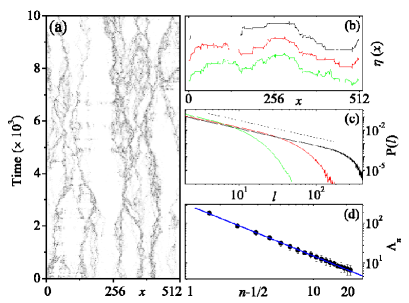
Some important features of the spatial structure are revealed by introducing the auxiliary fields, $\eta_{n}\equiv h_{n}-h_{1}$, measuring the relative growth of the $n$th LV with respect to the first one. In Fig. 2(b) we plot snapshots of $\eta_{n}(x,t)$ for backward LVs with $n=2,5$ and $20$ (similar profiles are observed for characteristic LVs). The profiles exhibit a distinctive structure organized in flat regions. These plateaus evolve so that their boundaries have an erratic motion as can be seen in Fig. 2(a). This spatial structure results from the fact that the dynamics of every LV is governed by Eq. (2) with the same ‘deterministic noise’. Spatial regions where $\partial_{x}\eta_{n}(x,t)\approx 0$ correspond to regions where the $n$th LV surface closely follows the first LV. This means that the dynamics specific of the $n$th LV surface is basically associated with that of the boundaries between plateaus. Since the first LV surface dynamics belongs to the KPZ universality class, the picture that immediately emerges from Fig. 2(b) is that the $n$th LV surface is, loosely speaking, “piecewise KPZ”.

The probability distributions of plateau lengths decay in good approximation as a power law $\mathrm{P}(l)\propto l^{-\gamma}$ for $l<\Lambda_{n}$ with $\gamma\approx 1.28\pm 0.10$ [Fig. 2(c)]. We find good evidence that the cut-off scales as $\Lambda_{n}\sim[L/(n-1/2)]^{\chi}$ where $\chi=1.29\pm 0.2$ [Fig. 2(d)]. There is some numerical uncertainty in the plateau and cut-off determination but we can estimate the average plateau length $\langle l_{n}\rangle\approx[L/(n-1/2)]^{0.75\pm 0.2}$.

Figure 3: (Color online) (a,b) Structure factors of $h_{n}$, $n=1,5,10,20,40$ from top to bottom, $L=1024$. (c,d) Data collapse through scaling relation (3) with fitting parameter $\theta=0.9\pm 0.1$.

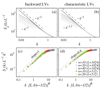
Spatial structure.- Let us now study the spatial correlations of the LV surfaces $h_{n}(x,t)$. We computed the stationary structure factor $S_{n}(k)=\lim_{t\to\infty}\langle\hat{h}_{n}(k,t)\hat{h}_{n}(-k,t)\rangle$, where $\hat{h}_{n}(k,t)=\sum_{x}\exp(ikx)h_{n}(x,t)$. One expects the first LV surface correlations to decay as $k^{-2}$ [Fig. 3(a,b)], in accordance with KPZ universality pik94 ; pik98 . Interestingly, the $n$th LV surface for $n>1$ also shows scale-invariant correlations $\sim k^{-2}$, but only up to a crossover length scale that depends on $n$. At long wavelengths correlations of LV surfaces, associated with backward and characteristic LVs, decay as $k^{-1}$ and $k^{-1.2}$, respectively (Fig. 3). This $1/k$-divergence indicates extremely weak long-range spatial correlations for both classes of LVs.

Numerical data for all LV surface spatial correlations in the stationary state [Fig. 3(a,b)] can be cast in a single scaling function as shown in Fig. 3(c,d):

$$S_{n}(k)L^{-1}k^{2}=g(k/\Bbbk_{n})$$ (3)

where $g(u)=\mathrm{const}$ for $u\gg 1$, and $g(u)\sim u^{\sigma}$ for $u\ll 1$, $\sigma=1$ and $\sigma=0.8$ for backward and characteristic LVs, respectively. The crossover wavelength is $\Bbbk_{n}\sim[L/(n-1/2)]^{-\theta}$, with $\theta=0.9\pm 0.1$, and gives a typical length scale $\ell_{n}\propto\Bbbk_{n}^{-1}$ for the $n$th LV surface, which immediately suggests to link $\ell_{n}$ with the average plateau length $\langle l_{n}\rangle$ introduced above.

Figure 4: Time evolution of $\phi_{10}(k,t)$ for (a) backward and (b) characteristic LVs ($L=512$).

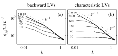
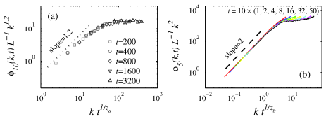
Space-time correlations.- For each $n$ we consider the field $h_{n}(x,t_{0}+t)-h_{n}(x,t_{0})$, measuring the relative growth of the $n$th LV between times $t_{0}$ to $t_{0}+t$ at a given point in space and whose structure factor we denote by $\phi_{n}(k,t)$. We run trajectories for a long time $t_{0}$ to allow a good projection into the attractor and then measure $\phi_{n}(k,t)$ at different times $t$. Figure 4(a) shows that backward LV surfaces for $n>1$ show long-range correlations $\sim 1/k$ already at very short times. We claim this is due to non-local information introduced by the Gram-Schmidt (orthogonalization) procedure that involves all LVs with $n^{\prime}<n$. Contrastingly, characteristic LV surfaces [Fig. 4(b)] exhibit excellent dynamic scaling properties. In this case the $n$th surface is uncorrelated —as indicated by a flat $\sim k^{0}$ structure factor— at scales $k\ll t^{-1/z}$, where $z$ is the dynamic exponent. As time proceeds correlations develop and extend over a correlation length $\xi\sim t^{1/z}$, as expected for typical dynamic scaling in kinetic surface roughening. Eventually, saturation occurs when $\xi$ reaches the system size $L$, and we recover the stationary correlations $\phi_{n}(k,t\rightarrow\infty)=S_{n}(k)$.

In agreement with the results for the static correlations, $S_{n}(k)$, discussed above, we can see two scaling regimes in Fig. 4(b) separated by the typical wavenumber $\Bbbk_{n}$. Curves corresponding to different times in Fig. 4(b) can be ‘collapsed’ into:

$$\phi_{n}(k,t)=k^{-\mu_{i}}c_{n}^{(i)}(kt^{1/z_{i}})$$ (4)

where the label $i\in\{a,b\}$ denotes the scaling region, above or below the crossover. On the one hand, for $t\gg\Bbbk_{n}^{-z_{b}}$, we find $\mu_{a}=1.2$ [Fig. 5(a)]. Our simulations indicate that the dynamic exponent $z_{a}=1$ is consistent with numerics on this range of scales for all $n$. This suggests a ballistic motion of the plateau boundaries of $\eta_{n}$. This small value of $z_{a}$ implies that the surface height correlates very rapidly once the correlation length reaches the intrinsic length scale $\ell_{n}$. Thus, the larger $n$ the sooner $\phi_{n}(k,t)$ reaches the asymptotic value. On the other hand, for $t\ll\Bbbk_{n}^{-z_{b}}$ we find $\mu_{b}=2$ [Fig. 5(b)]. Our simulations indicate —supported also by the computation of the surface growth exponent $\beta_{b}$ (not shown)— a slow continuous increase of the dynamic exponent with $n$ (for $n=1$, $z_{KPZ}=3/2$ for sufficiently large systems). Therefore, at short scales characteristic LV surface correlations propagate slightly more slowly when we look at larger $n$.

Figure 5: (Color online) Dynamic scaling through scaling relation (4). (a) Data collapse above the crossover with $\mu_{a}=1.2$ and $z_{a}=1$. Scaling shows up only for wavenumbers smaller than the intrinsic scale $k<\Bbbk_{10}\approx 0.13$, in agreement with the crossover picture. (b) Collapse below the crossover, $n=5$ (instead of $n=10$) has been used to obtain a larger region of scaling; $\mu_{b}=2$ and $z_{b}=1.75\pm 0.1$.

Observations and Outlook.- In our opinion characteristic LVs are more fundamental for a theoretical understanding of STC than the more commonly used (Gram-Schmidt) backward LVs. We have shown that they have strong localization properties, so that they generically localize in physical space, signaling regions where most unstable expanding directions concentrate at a given time. This suggests that characteristic LVs, rather than backward vectors, may play an important role in the hierarchical decomposition of STC egolf00 .

We conjecture that the dynamics of the $n$th characteristic LV surface for $n>1$ is described by a KPZ saddle solution: given a certain realization of the (deterministic) noise there should exist (measure zero) initial perturbations that evolve toward states whose space-time surface correlations scale with critical exponents that are not given by the standard KPZ universality class. This would correspond to the scaling $\sim k^{-1.2}$ for long wavelengths, $k<\Bbbk_{n}$, in Fig. 3(b). While solutions whose basin of attraction is a set of measure zero are irrelevant for stochastic equations, in deterministic chaos these may be fundamental solutions for the complete understanding of sensitive dependence in high-dimensional chaotic systems. In fact, it has recently been shown that the stochastic KPZ equation does exhibit this type of saddle solutions for noise realizations with suitable (and admittedly bizarre) correlations canet_moore07 . We have shown that, in statistical terms, the $n$th characteristic LV surface $h_{n}(x,t)$ differs from a genuine KPZ surface in an amount given by a field $\eta_{n}(x,t)$. It is not difficult to convince oneself that the step field corresponds to the nontrivial solutions (i.e. $\eta_{n}\neq\mathrm{const.}$) of the stochastic equation:

$$\partial_{t}\eta_{n}=(\partial_{x}\eta_{n})^{2}+\partial_{xx}\eta_{n}+2(\partial_{x}h_{1})(\partial_{x}\eta_{n}).$$ (5)

In a quite natural way the term $\partial_{x}\eta_{n}$ on the right hand side leads to solutions of the type shown in Fig. 2(b); plateaus of random spatial extent separated by boundaries moving erratically. We believe that Eq. (5) may indeed provide a mathematical tool to address questions like real-space structure of the dynamics of extended systems, space-time correlations in the propagation of disturbances, degree of localization of unstable directions, and extensivity and decomposition of STC.

Finally, we have found identical behavior in other CML models. In fact, our conclusions should be generic for LVs corresponding to LEs well above zero in systems whose first LV surface belongs to the KPZ universality class szendro_unpu . (This certainly should include all those systems reported in Ref. pik98 .) Although more research is needed to test the generality of our findings, in particular for continuous-time systems, our preliminary results with a minimal stochastic model ($\partial_{t}w=\zeta w+\partial_{xx}w$) confirm the universality of our results szendro_unpu .

Financial support from the Ministerio de Educación y Ciencia (Spain) under projects FIS2006-12253-C06-04 and CGL2004-02652/CLI is acknowledged. DP acknowledges support by MEC (Spain) through the Juan de la Cierva Programme.

References

- (1) J.-P. Eckmann and D. Ruelle, Rev. Mod. Phys. 57, 617 (1985).
- (2) T. Bohr, M. H. Jensen, G. Paladin, and A. Vulpiani, Dynamical Systems Approach to Turbulence (Cambridge, Cambridge, 1988).
- (3) E. Ott, Chaos in Dynamical Systems (Cambridge University Press, Cambridge, 1993).
- (4) C. Primo, I. G. Szendro, M. A. Rodríguez, and J. M. Gutiérrez, Phys. Rev. Lett. 98, 108501 (2007).
- (5) A. S. Pikovsky and J. Kurths, Phys. Rev. E 49, 898 (1994).
- (6) A. Pikovsky and A. Politi, Nonlinearity 11, 1049 (1998).
- (7) J. M. López, C. Primo, M. A. Rodríguez, and I. G. Szendro, Phys. Rev. E 70, 056224 (2004).
- (8) A. D. Sánchez, J. M. López, M. A. Rodríguez, and M. A. Matías, Phys. Rev. Lett. 92, 204101 (2004).
- (9) M. Kardar, G. Parisi, and Y.-C. Zhang, Phys. Rev. Lett. 56, 889 (1986).
- (10) G. Benettin, L. Galgani, A. Giorgilli, and J.-M. Strelcyn, Meccanica 15, 9 (1980).
- (11) A. Wolf, J. B. Swift, H. L. Swinney, and J. A. Vastano, Physica D 16, 285 (1985).
- (12) V. I. Oseledec, Trans. Moscow Math. Soc. 19, 197 (1968).
- (13) B. Legras and R. Vautard, in Predictability Vol. I, ECWF Seminar, edited by T. Palmer (ECMWF, Reading, UK, 1996), pp. 135–146.
- (14) S. V. Ershov and A. B. Potapov, Physica D 118, 167 (1998).
- (15) A. Trevisan and F. Pancotti, J. Atmos. Sci. 55, 390 (1998).
- (16) C. L. Wolfe and R. S. Samelson, Tellus 59A, 355 (2007).
- (17) F. Ginelli et al., arXiv:0706.0510v1 [nlin.CD].
- (18) D. A. Egolf, I. V. Melnikov, W. Pesch, and R. E. Ecke, Nature 404, 733 (2000).
- (19) L. Canet and M. A. Moore, Phys. Rev. Lett. 98, 200602 (2007).
- (20) I. G. Szendro, D. Pazó, M. A. Rodríguez, and J. M. López, to be published.