Resonant phenomena in extended chaotic systems subject to external noise: the Lorenz’96 model case

Abstract

We investigate the effects of a time-correlated noise on an extended chaotic system. The chosen model is the Lorenz’96, a kind of “toy” model used for climate studies. Through the analysis of the system’s time evolution and its time and space correlations, we have obtained numerical evidence for two stochastic resonance-like behavior. Such behavior is seen when both, the usual and a generalized signal-to-noise ratio function are depicted as a function of the external noise intensity or the system size. The underlying mechanism seems to be associated to a noise-induced chaos reduction. The possible relevance of these and other findings for an optimal climate prediction are discussed.

I Introduction

The last decades have witnessed a growing interest in the study of the effect of noise on dynamical systems. It was proved that, under some conditions, when a nonlinear dynamical system is subject to noise, new phenomena can arise, phenomena that only occur under the effect of such noise. All these phenomena are lump together under the name noise-induced phenomena. A few examples are: stochastic resonance in zero-dimensional and extended systems RMP ; extend1 ; extend2 , noise-induced transitions lefev , noise-induced phase transitions nipt1 ; nipt2 , noise-induced transport Ratch2 ; nipt3 , noise-sustained patterns ga93 ; ber , noise-induced limit cycle mangwio .

Clearly, some of the above indicated noise-induced phenomena occur in spatially extended systems, where another phenomena of great relevance exists: spatio-temporal chaos chaos00 . However, studies on the effect of noise on spatially extended chaotic systems are scarce chaos01 . There are studies on chaotic systems where the pseudo-random behavior of the system is the trigger of phenomena usually associated with the effect of a real stochastic process (see for instance rus ; deter ). Hence, we can refer to the presence of a deterministic noise, that is a pseudo-noisy behavior associated to the chaotic character of the system.

Among others, one of the most relevant and largely analyzed application of studies of chaos in extended systems corresponds to climate prediction. These kind of problems have been described by Lorenz Lor96-1 as falling into two categories. On one hand those which depend on the initial conditions, while on the other are those depending on the boundaries. However, both kind of prediction problems are affected by errors in the model equations used to approximately described the behavior of real systems.

In a recent work Lor96-3 , and with the aim to improve the limited weather predictability that results from a combination of initial conditions uncertainty and model error, it was presented a study of the effect of a stochastic parametrization in the Lorenz’96 model Lor96-1p ; Lor96-2 . It is well known that much of the current error in weather predictability derives from the practice of representing the effects of process occurring at unresolved scales by using simple forms of deterministic parametrization, attempting to summarize the effects of small-scale processes in terms of larger-scale, resolved, prognostic variables.

In this work, and with a similar objective as in a previously indicated paper Lor96-3 , we investigate the effect of a time-correlated noise on an extended chaotic system, analyzing the competence between the above indicated deterministic noise and a real stochastic process. In order to perform such a study we have chosen the Lorenz’96 model Lor96-1 . In spite of the fact that it is a kind of toy-model, at variance with the cases studied in chaos01 , it has a clear contact with real systems as it is of interest for the analysis of climate behavior and weather prediction Lor96-1p ; Lor96-2 ; Lor96-3 . In fact, this model has been heuristically formulated as the simplest way to take into account certain properties of global atmospheric models. To reach our objective, we have assumed that the only model parameter is time dependent and composed of two parts, a constant deterministic contribution plus a stochastic one.

Through the analysis of the system’s temporal evolution and its time and space correlations, we have obtained numerical evidence for two stochastic resonance-like (SR) RMP behaviors. Such behaviors are seen when both, the usual signal-to-noise ratio (SNR) and a generalized function $SNR_{glob}$ (that we call global SNR), are depicted as function of the external noise intensity or the system size. In accord with what was shown in previous works RMP , a SR phenomenon can occur in systems without external periodic forcing, but having an internal typical frequency. Hence, it seems reasonable to assume that the present resonances typically occur at frequencies corresponding to a system’s internal quasi-periodic behavior, as well as at an optimal system’s size. Finally, we discuss the possible relevance of these findings for climate prediction.

II The Model and Response Measures

II.1 The Model Lorenz’96

The equations corresponding to the Lorenz’96 model Lor96-1 ; Lor96-1p are

$$\dot{x}_{j}(t) = -x_{j-1}(x_{j-2}-x_{j+1})-x_{j}+F.$$ (1)

$$j = 1,2,3,\ldots,N,$$

where $\dot{x}_{j}(t)$ indicates the time derivative of $x_{j}(t)$. In order to simulate a scalar meteorological quantity extended around a latitude circle, we consider periodic boundary conditions: $x_{0}=x_{N},\,\,\,\,x_{-1}=x_{N-1}$.

As indicated before, the Lorenz’96 model Lor96-1 has been heuristically formulated as the simplest way to take into account certain properties of global atmospheric models. The terms included in the equation intend to simulate advection, dissipation and forcing respectively. In contrast with other toy models used in the analysis of extended chaotic systems and based on coupled map lattices, the Lorenz’96 system exhibits extended chaos ($F>9/8$), with a spatial structure in the form of moving waves Lor96-1 . The length of these waves is close to 5 spatial units. It is worth noting that the system has scaled variables with unit coefficients, hence the time unit is the dissipative decay time. In these units the group velocity of the waves is close to $v_{gr}=1.20$ implying a eastward propagation. If, as done by Lorenz, we associate the time unit to 5 days and the system size of 40 to the length of a latitude circle, we have a highly illustrative representation of a global model. If in addition we adjust the value of the parameter $F$ to give a reasonable signal to noise ratio (Lorenz considered $F=8$) the model could be most adequate to perform basic studies of predictability. Hence, within this framework, the signal analyzed in this paper would correspond to the passing of waves in a generic observational site, in what is a simple mimic of forecasting at an intermediate time range.

II.2 Stochastic contribution

As indicated before, here we assume that the model parameter $F$ becomes time dependent, and has two contributions, a constant and a random one

$$F_{j}(t)=F_{med}+\Psi_{j}(t),$$ (2)

with $\Psi_{j}(t)$ a dichotomic process. That is, $\Psi_{j}(t)$ adopts the values $\pm\Delta$, with a transition rate $\gamma$: each state ($\pm\Delta$) changes according to the waiting time distribution $\psi_{i}(t)\sim e^{-\gamma t}$. The noise intensity for this process is defined through vK ; Gar $\xi=\frac{\Delta^{2}}{2\,\gamma}$.

II.3 System Response

As a measure of the SR system’s response we have used the signal-to-noise ratio (SNR) RMP . To obtain the SNR we need to previously evaluate $S(\omega)$, the power spectral density (psd), defined as the Fourier transform of the correlation function vK ; Gar

$$S(\omega)=\int_{-\infty}^{\infty}e^{i\omega\tau}\langle x_{j}(0)x_{j}(\tau)\rangle\,d\tau,$$ (3)

where $\langle\,\,\,\rangle$ indicates the average over realizations. As we have periodic boundary conditions simulating a closed system, $\langle x_{j}(0)x_{j}(\tau)\rangle$ has a homogeneous spatial behavior. Hence, it is enough to analyze the response in a single site.

We consider two forms of SNR. In one hand the usual SNR measure at the resonant frequency $\omega_{o}$ (that is, in fact, at the frequency associated to the highest peak in $S(\omega)$) is

$$SNR=\frac{\int^{\omega_{o}+\sigma}_{\omega_{o}-\sigma}d\varpi S(\varpi)}{\int^{\omega_{o}+\sigma}_{\omega_{o}-\sigma}d\varpi S_{back}(\varpi)},$$ (4)

where $2\sigma$ is a very small range around the resonant frequency $\omega_{o}$, and $S_{back}(\omega)$ corresponds to the background psd. On the other hand we consider a global form of the SNR ($SNR_{glob}$) defined through

$$SNR_{glob}=\frac{\int^{\omega_{max}}_{\omega_{min}}d\omega S(\omega)}{\int^{\omega_{max}}_{\omega_{min}}d\omega S_{back}(\omega)},$$ (5)

where $\omega_{min}$ and $\omega_{max}$ define the frequency range where $S(\omega)$ has a reach peak structure (with several resonant frequencies).

III Results

We have analyzed the typical behavior of trajectories as $x_{1}(t)-x_{med-T}$, where $x_{med-T}$ is the time average. It is worth commenting that when the Lorenz 96 system evolves without external noise (that is $F_{j}(t)$ is constant), the time evolution shows a random-like behavior, with the main feature that the amplitude of the oscillator is constant over all the time. However, when the system is subject to a random force as described in Eq. (2), the temporal response decays, due to the fact that the interaction between the intrinsic evolution and the external noise produces a dissipative contribution on the system. Hence the system’s time evolution consists of a transitory regime and a stationary one. This was analyzed through the behavior of the “decay” of $\langle x_{1}(t)-x_{med-T}\rangle$. We assumed that this decay can be adjusted by an exponential law. The decay parameter ($\lambda$) only depends on $F_{med}$ and it does not depend neither on the system size nor on the noise intensity. This analysis is relevant when studying the effects of noise on the stationary regime. From those results it was possible to anticipate, and approximately identify, the existence of two regimes: a weak or undeveloped chaos for $F_{med}<6.0$, and strong or completely developed chaos for $F_{med}>6.0$.

The typical numbers we have used in our simulations are: averages over $10^{3}$ histories, and $\sim 10^{4}$ simulation time steps (within the stationary regime, see later).

We have evaluated the psd $S(\omega)$ in a standard way. Figure 1-a shows the typical form of the psd $S(\omega)$ for a couple of values of $F_{med}$ ($F_{med}=4.5,7.8$) and for a noise intensity $\Delta=0.1$ ($\xi=5\times 10^{-4}$). The figure shows a rich peak structure within the interval $0.22<\omega<1.3$. It is worth to comment that the frequencies associated to the different peaks seems to correspond to the harmonics of the main (or first) peak frequency. In Fig. 1-b, we show the form of $S(k)$, the associated spatial spectrum. Here we depict the spectrum for fixed values of the system’s size ($N=256$), and noise intensity ($\Delta=0.001$ and $\gamma=10$), and different values of $F_{med}$. The independence of the position of the peak (indicating a single spatial structure of wavelength $k/2\pi=0.2$) is apparent. However there is a strong dependence on the peak intensity when varying $F_{med}$, from a net peak for underdeveloped chaos ($F_{med}=5$) to a reduced peak for well developed chaos ($F_{med}=8$). It is worth here remarking that there is no dependence (or eventually a very weak one) of this behavior on the noise intensity.

Figure 1: (a) $S(\omega)$ for a couple of values of $F_{med}$ ($F_{med}=4.5,7.8$) and for a small noise intensity ($\xi=5\times 10^{-4}$, $\Delta=0.1$ and $N=128$). (b) Spatial spectrum for $N=256$, $\Delta=0.001$ and $\gamma=10$, for several values of $F_{med}$: continuous line $F_{med}=5$, dashed $F_{med}=6$, dotted $F_{med}=7$ and dash-dotted $F_{med}=8$ .

Figure 2 shows the dependence of $SNR_{glob}$ –for a space-temporal noise– on $\Delta$ for fixed values of $N$ and a couple of values of $F_{med}$. It shows a peak for $\Delta\sim 6-7\times 10^{-3}$, that corresponds to the fingerprint of the more usual form of SR. The insert shows the same case but for $SNR$.

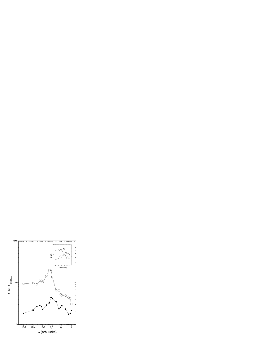
Figure 2: $SNR_{glob}$ vs $\Delta$, for fixed values of $N=64$ and $\gamma=10$; and a couple of values of $F_{med}$: white circles $F_{med}=5$, black squares $F_{med}=6$. The insert shows the behavior of the usual $SNR$ for the same cases.

The analysis of the dependence of $SNR_{glob}$ on $F_{med}$ have also shown the existence of the previously indicated two regimes: a weak or undeveloped chaos for $F_{med}<6.0$, and a strong or completely developed chaos for $F_{med}>6.0$. Those regimes are characterized by the existence of well defined peaks in the psd, in the former case, and a less defined peak structure in the latter case, as seen in Fig. 1a .

It is worth to detach the strong similarities in the behavior of $SNR$ and $SNR_{glob}$ –which becomes apparent when comparing the main Fig. 2 with its insert– indicating that the second one is an adequate and more versatile measure to characterize the system’s response. Hence, due to the clearness in the determination of $SNR_{glob}$ (compared with the difficulties for a correct determination of $SNR$ for large values of $F_{med}$) in what follows we adopt it for the system’s analysis.

In Fig. 3 we depict the dependence of $SNR_{glob}$ on $N$, for the case of space-temporal noise, for fixed values of $\Delta=0.1$ and $\gamma=5$ ($\xi=0.001$) and a couple of values of $F_{med}$. The existence of the peak at $N\sim 60$ for $F_{med}=5.0$ is apparent. In addition, we observe an increase of $SNR_{glob}$ for large values of $N$. However, for $F_{med}=6.0$, the peak has disappeared, as well as the increase with larger values of $N$. The presence of the peak at $N\sim 60$ indicates a kind of system-size stochastic-resonance (SSSR) sssr . The insert shows the same case but for $SNR$. Again, as indicated above, the nice agreement between the behavior of $SNR_{glob}$ and that of $SNR$.

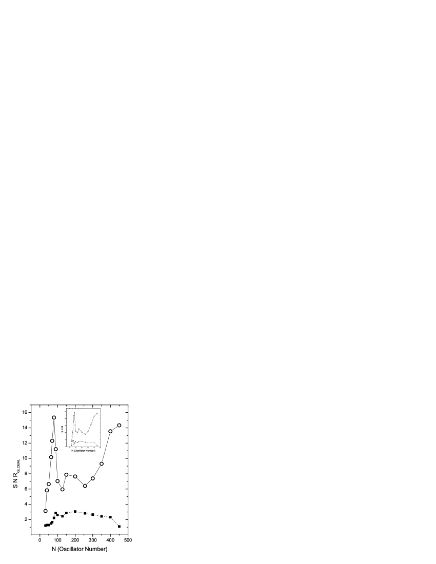
Figure 3: $SNR_{glob}$ vs $N$, for fixed values of $\Delta=0.1$ and $\gamma=5$ ($\xi=0.001$), and a couple of values of $F_{med}$: white circles $F_{med}=5$, black squares $F_{med}=6$. The insert shows the behavior of the usual $SNR$ for the same cases.

The figures clearly show that the system’s response (SNR) is stronger when the system is in the underdeveloped chaos range than when it is in the highly-developed chaos one. Our results also show that the main resonant frequency does not depend on the noise intensity, system size, or correlation rate.

We want to close this section commenting that the SR phenomena found here looks similar to the so called internal signal SR int . In previous studies it was shown that in some systems having an internal typical frequency, SR can occur not only at the frequency of an external driving signal, but at the frequency corresponding to the internal periodic behavior int . Regarding the present mechanism of SR, what we can indeed comment is that the increase in the SNR is related not to a reinforcement of the peak high respect to the noisy background at a given frequency, but with a reduction of the pseudo (or deterministic) noisy background when turning on the real noise. That is, the interplay between “real” noise and “deterministic” noise conforms a kind of noise-induced chaos reduction. Figure 4 shows, for fixed values of $F$ and $\gamma$, the behavior of $S(\omega)$ in both cases: with ($\Delta\neq 0$) and without noise ($\Delta=0$). The above indicated reduction trend, as the real noise is turned on, is apparent. However, the present mechanism is not completely clear so far, and requires further studies.

Figure 4: $S(\omega)$ with and without external noise, for $F=5$ and $\gamma=10$. Continuous line $\Delta=0$, dot-line $\Delta=0.1$.

IV Conclusions

We have investigated the effect of a time-correlated noise on an extended chaotic system, analyzing the competence between the indicated deterministic or pseudo-noise and the real random process. For our study we have chosen the Lorenz’96 model Lor96-1 that, in spite of the fact that it is a kind of toy model, is of interest for the analysis of climate behavior Lor96-2 ; Lor96-3 . It worth remarking that it accounts in a simple way of the spatial structure of geostrophic waves and the dynamics of tropical winds. The time series obtained at a generic site $x_{i}(t)$ mimics the passing of such waves, which is in fact a typical forecast event. We have assumed that the unique model parameter $F$, is time dependent and composed of two parts, a constant deterministic, and a stochastic contribution in a spatial-temporal form.

We have done a thorough analysis of the system’s temporal evolution and its time and space correlations. From our results it is clear that, using two complementary SNR measures, a usual and a global one, we have obtained numerical evidence for two SR-like behaviors. In one hand a “normal” SR phenomenon occur at frequencies that seem to correspond to a system’s quasi-periodic behavior. On the other hand, we have found a SSSR-like behavior, indicating that there is an optimal system size for the analysis of the spatial system’s response. As indicated before, the effect of noise is stronger when the chaos is underdeveloped.

We argue that these findings are of interest for an optimal climate prediction. It is clear that the inclusion of the effect of an external noise, that is a stochastic parametrization of unknown external influences, could strongly affect the deterministic system response, particularly through the possibility of an enhanced system’s response in the form of resonant-like behavior. It is worth here remarking the excellent agreement between the resonant frequencies and wave length found here, and the estimates of Lorenz Lor96-1p .

The effect of noise is weak respect to changes in the spatial structure, with the main frequencies remaining unaltered, but it is strong concerning the strength of the “self-generated” deterministic noise. In fact, in such a system and at the resonant frequencies, forecasting could be improved by the external noise due to the effect of suppression of the self-generated chaotic noise. The detailed analysis of such an aspect will be the subject of a forthcoming study nos1 .

References

- (1) L. Gammaitoni, P. Hänggi, P. Jung and F. Marchesoni, Rev. Mod. Phys. 70, 223 (1998).
- (2) J. F. Lindner, B. K. Meadows, W. L. Ditto, M. E. Inchiosa and A. Bulsara, Phys. Rev. E 53, 2081 (1996);
- (3) H. S. Wio, Phys. Rev. E 54, R3045 (1996); F. Castelpoggi and H. S. Wio, Europhys. Lett. 38, 91 (1997); F. Castelpoggi and H. S. Wio, Phys. Rev. E 57, 5112 (1998); S. Bouzat and H. S. Wio, Phys. Rev. E 59, 5142 (1999); H. S. Wio, S. Bouzat and B. von Haeften, in Proc. 21st IUPAP International Conference on Statistical Physics, STATPHYS21, A.Robledo and M. Barbosa, Eds., published in Physica A 306C 140-156 (2002).
- (4) W. Horsthemke and R. Lefever, Noise-Induced Transitions: Theory and Applications in Physics, Chemistry and Biology, (Springer, Berlin, 1984).
- (5) C. Van den Broeck, J. M. R. Parrondo and R. Toral, Phys. Rev. Lett. 73, 3395 (1994); C. Van den Broeck, J. M. R. Parrondo, R. Toral and R. Kawai, Phys. Rev. E 55, 4084 (1997).
-
(6)
S. Mangioni, R. Deza, H. S. Wio and R. Toral,
Phys. Rev. Lett. 79, 2389 (1997);
S. Mangioni, R. Deza, R. Toral and H. S. Wio, Phys. Rev. E 61, 223 (2000). - (7) P. Reimann, Phys. Rep. 361, 57 (2002); R. D. Astumian and P. Hänggi, Physics Today, 55 (11) 33 (2002).
- (8) P. Reimann, R. Kawai, C. Van den Broeck and P. Hänggi, Europhys. Lett. 45, 545 (1999); S. Mangioni, R. Deza and H.S. Wio, Phys. Rev. E 63, 041115 (2001).
- (9) J. García-Ojalvo, A. Hernández-Machado and J. M. Sancho, Phys. Rev. Lett. 71, 1542 (1993); J. García-Ojalvo and J. M. Sancho, Noise in Spatially Extended Systems (Springer-Verlag, New York, 1999).
- (10) B. von Haeften and G. Izús, Phys. Rev. E 67, 056207 (2003), G. Izús, P. Colet, M. San Miguel and M. Santagiustina, Phys. Rev. E 68, 036201 (2003).
- (11) S. Mangioni and H. S. Wio, Phys. Rev. E 67, 056616 (2003).
- (12) T. Bohr, M.H. Jensen, G. Paladin and A. Vulpiani, Dynamical Systems Approach to Turbulence, (Cambridge U.P., Cambridge, 1998).
- (13) J.M. Gutiérrez, A. Iglesias and M.A. Rodríguez , Phys. Rev. Lett. 48, 2507 (1993); H. Wang and Q. Ouyang, Phys. Rev. E 65 046206 (2002); G. A. Gottwald and I. Melbourne, Physica D 212, 100 (2005); G. Ambika, K. Menon and K.P. Harikrishnan, Europhys. Lett. 73, 506 (2006).
- (14) V. S. Anishchenko, A. B. Neiman and M. A. Safanova, J. Stat. Phys. 70, 183 (1993); V. S. Anishchenko, M. A. Safanova and L. O. Chua, Int. J. Bifurcation and Chaos Appl. Sci. Eng. 4, 441 (1994).
- (15) D. Hennig, L. Schimansky-Geier and P. Hänggi, Europhys. Lett. 78, 20002 (2007).
- (16) D. S. Wilks, Quaterly J. of the Royal Meteor. Soc. B 131, 389 (2005)
- (17) E. N. Lorenz, The essence of chaos, (U.Washington Press, Washington, 1996).
- (18) E. N. Lorenz and K. A. Emanuel, J. Atmosph. Sci. 55, 399 (1998).
- (19) D. Orrell, J. Atmosph. Sci. 60, 2219 (2003)
- (20) N. van Kampen; Stochastic Processes in Physics and Chemistry, (North Holland, 1982)
- (21) C. W. Gardiner; Handbook of Stochastic Methods, 2nd Ed. (Springer-Verlag, Berlin, 1985).
- (22) H. Gang, T. Ditzinger, C.Z. Ning and H. Haken, Phys. Rev. Lett. 71, 807 (1993); S. Zhong and H. Xin, J. Phys Chem. 104, 297 (2000); A. F. Rosenfeld, C. J. Tessone, E. Albano and H. S. Wio, Phys. Lett. 280, 45 (2001).
- (23) B. von Haeften, G. G. Izús and H. S. Wio, Phys. Rev. E 72, 021101 (2005).
- (24) J. A. Revelli, M. A. Rodriguez and H. S. Wio, to be submited to Europ. Phys. J. B.