Controlling Secondary Structures of Bio-Polymers with Hydrogen-Like Bonding

Abstract

We present results for a lattice model of bio-polymers where the type of $\beta$-sheet formation can be controlled by different types of hydrogen bonds depending on the relative orientation of close segments of the polymer. Tuning these different interaction strengths leads to low-temperature structures with different types of orientational order. We perform simulations of this model and so present the phase diagram, ascertaining the nature of the phases and the order of the transitions between these phases.

I Introduction

The transition of a flexible macromolecular chain from a random-coil conformation to a globular compact form, called coil-globule transition, has been a subject of extensive theoretical and experimental studies baysal2003 . Generally, polymers in a good solvent are modelled by random walks with short-range repulsion (excluded volume). Polymers undergoing a coil-globule transition are then modelled by adding an additional short-range attraction. This short-range attraction is both due to an affinity between monomers and solvent molecules, affecting the solvability of a polymer, and also due to intra-molecular interactions between different monomers, for example due to van-der-Waals forces. The canonical lattice model orr1946 ; bennett1998 for this transition is given by interacting self-avoiding walks, in which self-avoiding random walks on a lattice are weighted according to the number of nearest-neighbour contacts (non-consecutively visited nearest-neighbour lattice sites).

It is recognised that in biological systems, e.g. proteins, the most relevant contribution to monomer-monomer-interactions is due to hydrogen bonds. These hydrogen bonds can only form if neighbouring segments are aligned in a certain way, resulting in an interaction that is strongly dependent on the relative orientation of segments. This type interaction plays a leading role in the formation of secondary protein structures such as $\alpha$-helices and $\beta$-sheets pauling1951 . In this paper, we introduce a model for controlling the type of orientational order of these structures.

In bascle1993 , Bascle et al introduced a lattice model of polymers interacting via hydrogen bonds, in which hydrogen bonds were mimicked by an interaction between two nearest-neighbour lattice sites which belong to two straight segments of the polymer. This was treated in the context of Hamiltonian walks in a mean-field approach, and they predicted a first-order transition between an anisotropic ordered phase and a molten phase. Later, Foster and Seno introduced this type of interaction to a model of self-avoiding walks foster2001 . They analyzed it using transfer-matrix techniques in two dimensions, where a first-order transition between a folded polymer crystal and a swollen coil was found. Subsequently, a variant of this model was introduced by Buzano and Pretti buzano2002 , where the interaction is defined between parallel nearest-neighbour bonds, independent of the straightness required in bascle1993 , arguing that these should better take into account the contribution of fluctuating bonds, which may be formed even in relatively disordered configurations. The authors studied this interacting-bond model and the one introduced by Foster and Seno on the square and simple cubic lattice using the Bethe approximation. They found a first-order transition in the Foster-Seno model in two and three dimensions, confirming and extending results in foster2001 . In contrast to this, they found two transitions in the interacting-bond model, a second-order $\theta$-transition from a swollen coil to a collapsed molten globule and then a first-order transition to a folded polymer crystal. In a later paper buzano2003 , they introduced a competing isotropic interaction and studied its effect in three dimensions using the Bethe approximation. They found a phase diagram with three different phases (swollen coil, collapsed molten globule, folded polymer crystal), similar to that of collapsing semi-stiff polymers bastolla1997 .

In this work we generalize the Foster-Seno model to distinguish between nearest-neighbour contacts of parallel and orthogonal straight segments (see Figure 1) and assign interactions of different strengths to these two types of contacts, investigating it with Monte-Carlo simulations using the the FlatPERM algorithm prellberg2004 . We begin by simulating the Foster-Seno model and confirm the theoretical picture presented above foster2001 ; buzano2003 . We then consider our extended model (in three dimensions). We find evidence for two differently structured folded phases, depending on whether the parallel or orthogonal interactions dominate. The transition between the swollen coil and each of the two collapsed ordered crystals is first-order. We investigate the structure of these two low-temperature phases. For strong parallel interactions long segments of the polymer align, whereas for strong orthogonal interactions the polymer forms alternating orthogonally layered $\beta$-sheets.

II Model and simulations

A polymer is modelled as an $n$-step self-avoiding walk on the simple cubic lattice with interactions $-\varepsilon_{p}$ and $-\varepsilon_{o}$ for nearest-neighbour contacts between parallel and orthogonal straight segments of the walk, as shown in Figure 1. Here, a segment is defined as a site along with the two adjoining bonds visited by the walk, and we say that a segment is straight if these two bonds are aligned. The restriction of this model to $\varepsilon_{o}=\varepsilon_{p}$ is the simple generalisation of the Foster-Seno model, which was originally defined on a square lattice, to three dimensions.

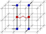
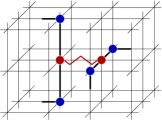
parallel (p)                            orthogonal (o)

Figure 1: The two types of nearest-neighbour contacts between two straight segments of the polymer: parallel segments (left) with interaction $-\varepsilon_{p}$, and orthogonal segments (right) with interaction $-\varepsilon_{o}$. In two dimensions, only parallel interactions are possible.

The total energy for a polymer configuration $\varphi_{n}$ with $n+1$ monomers (occupied lattice sites) is given by

$$E_{n}(\varphi_{n})=-m_{p}(\varphi_{n})\varepsilon_{p}-m_{o}(\varphi_{n})\varepsilon_{o}$$ (1)

depending on the number of non-consecutive parallel and orthogonal straight nearest-neighbour segments $m_{p}$ and $m_{o}$, respectively, along the polymer. For convenience, we define

$$\beta_{p}=\beta\varepsilon_{p}\mbox{ and }\beta_{o}=\beta\varepsilon_{o}\mbox{,}$$ (2)

where $\beta=1/k_{B}T$ for temperature $T$ and Boltzmann constant $k_{B}$. The partition function is given by

$$Z_{n}(\beta_{p},\beta_{o})=\sum_{m_{p},m_{o}}C_{n,m_{p},m_{o}}\;e^{\beta_{p}m_{p}+\beta_{o}m_{o}}$$ (3)

with $C_{n,m_{p},m_{o}}$ being the density of states. We have simulated this model using the FlatPERM algorithm prellberg2004 . The power of this algorithm is the ability to sample the density of states uniformly with respect to a chosen parametrisation, so that the whole parameter range is accessible from one simulation. In practice, we have also performed multiple independent simulations to further reduce errors. The natural parameters for this problem are $m_{p}$ and $m_{o}$, and the algorithm directly estimates the density of states $C_{n,m_{p},m_{o}}$ for all $n\leq n_{max}$ for some fixed $n_{max}$ and all possible values of $m_{p}$ and $m_{o}$. Canonical averages are performed with respect to this density of states. As we need to store the full density of states, we only perform simulations up to a maximal length of $n_{max}=128$, due to a memory requirement growing as $n^{3}$. To reduce the error, we have taken averages of ten independent runs each. Each run has taken approximately 3 months on a 2.8GHz PC to complete.

Fixing one of the parameters $\beta_{p}$ and $\beta_{o}$ reduces the size the histogram, and enables us to perform simulations of larger systems, as the memory requirement now grows as $n^{2}$. Fixing $\beta_{o}$, say, the algorithm directly estimates a partially summed density of states

$$\widehat{C}_{n,m_{p}}(\beta_{o})=\sum\limits_{m_{o}}C_{n,m_{p},m_{o}}e^{\beta_{o}m_{o}}\;.$$ (4)

In this way, we can simulate lengths up to $n_{max}=1024$ at fixed $\beta_{o}$. In a similar fashion, we also consider the diagonal $\beta_{p}=\beta_{o}=\beta$, which is equivalent to considering the partially summed density of states

$$\widetilde{C}_{n,m}=\sum\limits_{m_{o}+m_{p}=m}C_{n,m_{p},m_{o}}\;.$$ (5)

To reduce the error for our runs up to $n=1024$, we have taken averages of ten independent runs each. Each run has taken approximately 2 months on a 2.8GHz PC to complete.

III Results

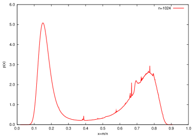
Figure 2: Internal energy density distributions for the two-dimensional Foster-Seno model at the value of $\beta$ for which the fluctuations are maximal, length $1024$.

Before presenting the findings for our model, we briefly discuss the results of simulations of the Foster-Seno model in two dimensions. We find a first-order transition between a swollen coil and ordered collapsed phase in agreement with Foster and Seno foster2001 . Figure 2 shows the internal density distribution at $\beta=\beta_{c}=1.04$, where the specific heat is maximal. This distribution is clearly bimodal, and finite-size scaling supports the conclusion that the transition is first-order. Our estimate of $\beta_{c}=1.04$ is close to the value $1.00(2)$ obtained by Foster and Seno foster2001 from transfer matrix calculations. The low temperature phase is an ordered $\beta$-sheet type phase.

For the three-dimensional model, we have explored the full two-variable phase space $(\beta_{p},\beta_{o})$ by using a two-parameter FlatPERM simulation of the model for lengths up to 128. We performed $10$ independent simulations to ensure convergence and understand the size of the statistical error in our results. As in previous work krawczyk2005a ; krawczyk2005b , we found the use of the largest eigenvalue of the matrix of second derivatives of the free energy with respect to the parameters $\beta_{p}$ and $\beta_{o}$ most advantageous to show the fluctuations in a unified manner. Figure 3 displays a density plot of the size of fluctuations for $0\leq\beta_{p},\beta_{o}\leq 2$. It suggests the presence of three thermodynamic phases separated by three phase transition lines meeting at a single point. For small values of $\beta_{p}$ and $\beta_{o}$, we expect the model to be in the excluded volume universality class of swollen polymers, since at $\beta_{p}=\beta_{o}=0$ the model reduces to the simple self-avoiding walk. The question arises as to the nature of the phases for large $\beta_{p}$ with $\beta_{o}$ fixed and for large $\beta_{o}$ with $\beta_{p}$ small, and the type of transitions between each of the phases.

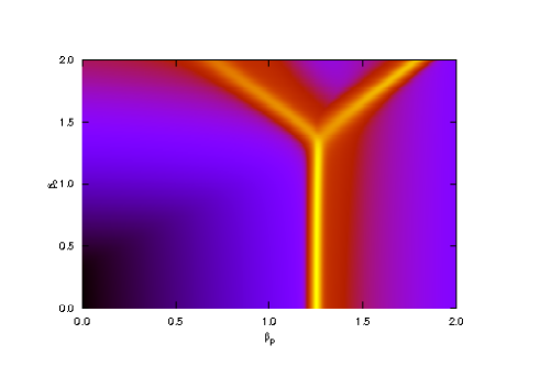
Figure 3: This is a density plot of the logarithm of the largest eigenvalue of the matrix of second derivatives of the free energy with respect to $\beta_{p}$ and $\beta_{o}$ at $n=128$. The lighter the shade the larger the value.

We find evidence for a strong collapse phase transition when increasing $\beta_{p}$ for fixed $\beta_{o}\lesssim 1.38$. Corrections to scaling at lengths $n\leq 128$ make it difficult to identify the nature of the transition. The location of the transition seems independent of the value of $\beta_{o}$ and is located at $\beta_{p}\approx 1.25$ for length $n=128$; this is taken from the location of the peak of the fluctuations. Since our data indicate that this transition occurs for $\beta_{o}\lesssim 1.38$ at $\beta_{p}\approx 1.25$, it follows that the diagonal line $\beta_{o}=\beta_{p}$ crosses this transition line. Configurations in the collapsed phase are rich in parallel contacts; we shall discuss further details of the collapsed phase below.

The situation changes significantly for $\beta_{o}\gtrsim 1.38$. When we start from the swollen phase at fixed $\beta_{o}>1.38$ and increase $\beta_{p}$ we see evidence for a strong phase transition to a different collapsed phase, in which orthogonal contacts are expected to play an important role. Further increase of $\beta_{p}$ leads to another strong transition to the parallel-contact rich phase. We investigate the transition between the swollen coil and the orthogonal-contact rich phase by considering the line $\beta_{p}=1.0$. Figure 4 shows a bimodal internal energy distribution at the maximum of the fluctuations in $m_{o}$ for length $n=128$, indicating the presence of a first-order transition.

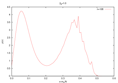
Figure 4: A plot of the internal energy distribution in $m_{o}$ at $\beta_{p}=1.0$ for length $n=128$ at values of $\beta_{o}$ for which the fluctuations in $m_{o}$ are maximal.

Combining the evidence above, we conjecture the phase diagram shown in Figure 5, having three phases and three transition lines that meet at a triple point located at $(\beta^{t}_{p},\beta^{t}_{o})\approx(1.25,1.38)$ for length $n=128$. By considering the location of this point for different lengths $n$, we conclude that its estimate is affected by strong finite-size corrections to scaling.

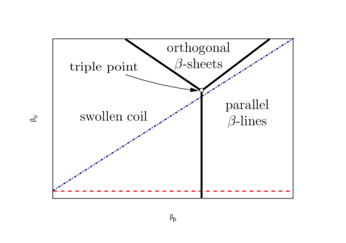
Figure 5: This figure represents our conjectured schematic phase diagram. The phases boundaries are marked by black lines. The dotted-dashed (blue) and dashed (red) lines denote the lines along which we have performed one-parameter simulations.

To further elucidate the nature of the phase transitions and the structure of the low-temperature phases, we perform simulations for larger system sizes for the two lines $\beta_{o}=0$ and $\beta_{o}=\beta_{p}$, using one-parameter FlatPERM simulations for lengths up to $n=1024$, averaged over ten independent simulations each. We begin by considering $\beta_{o}=0$. The peak of the specific heat occurs at $\beta_{p}=0.996$ for $n=1024$, which we note is shifted away from the value at length $n=128$ and reflects the presence of strong corrections to scaling. The distribution of $m_{p}$ at this point is shown in Figure 6; we observe a clear bimodal distribution with well-separated peaks and which ranges over fourteen orders of magnitude, convincingly supporting the conclusion of a first-order phase transition. Similarly, along the line $\beta=\beta_{o}=\beta_{p}$ we find a single peak of the specific heat, located at $\beta_{p}=0.998$ for $n=1024$. The distribution of $m=m_{o}+m_{p}$ at this point displays the same characteristics as the transition on the line $\beta_{o}=0$ described above. Our investigations of the transition between the two collapsed phases were not conclusive, as it is difficult to do simulations at very low temperatures. While we expect there to be a first order phase transition between the two collapsed phase we were unable to verify this.

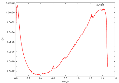
Figure 6: Internal energy density distributions of $m_{p}$ at $\beta_{o}=0$ and $\beta_{p}=0.996$ for length $1024$.

To delineate the nature of the two collapsed phases, we have randomly sampled typical configuration for each: two of these are shown in Figure 7. In each case we have used $\beta_{p}>0$, where parallel contacts are attractive. For large $\beta_{p}$, we have a parallel contact rich phase, and typical configurations have lines of monomers arranged in parallel. In Figure 7, there is a typical configuration for $(\beta_{p}=1.8,\beta_{o}=1.0)$, which demonstrates these parallel $\beta$-lines. For large $\beta_{o}$, orthogonal contacts play an important role. A typical configuration for $(\beta_{p}=1.3,\beta_{o}=1.9)$ consists of parallel lines arranged in $\beta$-sheets, which are layered orthogonally. The entropy of the phase consisting out of orthogonal $\beta$-sheets is lower than the entropy of the phase consisting out of collection of parallel lines, which explains why the collapse-collapse transition line is shifted away from the diagonal. Clearly the formation of $\beta$-sheets is dependent on $\beta_{p}$ being positive (attractive parallel) interactions.

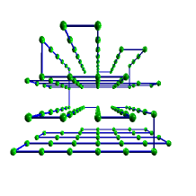
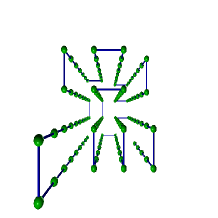
Figure 7: Typical configurations for the two different collapsed phases, sampled at $(\beta_{p}=1.3,\beta_{o}=1.9)$ (left) and at $(\beta_{p}=1.8,\beta_{o}=1.0)$ (right).

In conclusion, we have demonstrated the intriguing possibility of building a secondary structure in proteins, which involves layered $\beta$-sheets structures interacting in two different ways. Depending on the modelling of the interactions we distinguish $\beta$-sheets that align parallel or orthogonal to each other, which leads to two different phases, and secondary structures. There remains an interesting theoretical question as to the behaviour of the system when the parallel interactions are repulsive but the orthogonal interactions are highly attractive.

Financial support from the Australian Research Council and the Centre of Excellence for Mathematics and Statistics of Complex Systems is gratefully acknowledged by the authors.

References

- (1) B. M. Baysal and F. E. Karasz, Macromol. Theory Simul. 12 627 (2003)
- (2) W. J. C. Orr , Trans. Faraday Soc. 42 12 (1946)
- (3) D. Bennett-Wood et al, J. Phys. A 31 4725 (1998)
- (4) L. Pauling and R. B. Corey, PNAS 37 235,251,272,729 (1951)
- (5) J. Bascle, T. Garel and H. Orland, J. Physique II 3 245 (1993)
- (6) D. Foster and F. Seno, J. Phys. A 34 9939 (2001)
- (7) C. Buzano and M. Pretti, J. Chem. Phys. 117 10360 (2002)
- (8) C. Buzano and M. Pretti, Mol. Cryst. Liq. Cryst. 398 23 (2003)
- (9) U. Bastolla and P. Grassberger, J. Stat. Phys. 89 1061 (1997)
- (10) T. Prellberg and J. Krawczyk, Phys. Rev. Lett. 92 120602 (2004)
- (11) J. Krawczyk, A. L. Owczarek, T. Prellberg and A. Rechnitzer, JSTAT P05008 (2005)
- (12) J. Krawczyk, A. L. Owczarek, T. Prellberg and A. Rechnitzer, Europhys. Lett. 70 726 (2005)