$x$-Evolution of Phenomenological Dipole Cross Sections

Abstract

Deep inelastic scattering at small $x$ can be described very effectively using saturation inspired dipole models. We investigate whether such models are compatible with the numerical solutions of the Balitsky-Kovchegov (BK) equation which is expected to describe the nonlinear evolution in $x$ of the dipole cross section. We find that the BK equation yields results that are qualitatively different from those of phenomenological studies. Geometric scaling is recovered only towards asymptotic rapidities. In this limit the value of the anomalous dimension $\gamma(r,x)$ at the saturation scale approaches approximately $0.44$, in contrast to the value $0.63$ commonly used in the models.

At small $x$, deep inelastic scattering (DIS) can be described as the scattering of a color dipole, which the photon fluctuates into, off the proton [2]. The linear BFKL equation, which describes the dipole-proton interaction in terms of gluon ladders, predicts an exponential growth of the corresponding cross section as $\log 1/x$ increases, potentially violating unitarity. Hence, interactions between BFKL gluon ladders may become important, which leads to a nonlinear evolution approximately described by the Balitsky-Kovchegov (BK) equation [3]. As a consequence of the nonlinearity, the dipole cross section saturates with decreasing $x$, thereby offering a resolution to the unitarity problem. The inclusive HERA data at low $x$ ($x\raisebox{-4.0pt}{$\,\stackrel{{\scriptstyle\textstyle<}}{{\sim}}\,$}0.01$) could be described well by a dipole cross section of the form $\sigma=\sigma_{0}N_{\rm GBW}(r,x)$, where the scattering amplitude $N_{\rm GBW}$ is given by [4]

$$N_{\rm GBW}(r,x)=1-\exp\left[-\tfrac{1}{4}r^{2}Q_{s}^{2}(x)\right],$$ (1)

${r}$ denotes the transverse size of the dipole, $\sigma_{0}\simeq 23\;{\rm mb}$ and the $x$-dependence of the saturation scale is given by $Q_{s}(x)=1\,{\rm GeV}\,(x_{0}/x)^{\lambda/2}$, where $x_{0}\simeq 3\times 10^{-4}$ and $\lambda\simeq 0.3$. The scattering amplitude depends on $x$ and $r$ through the combination $r^{2}Q_{s}^{2}(x)$ only, which is known as geometric scaling and leads to the prediction that the structure function $F_{2}$ is a function of $Q^{2}/Q_{s}^{2}(x)$ only. This prediction was checked in a model independent way [5] and holds widely even though the GBW model (1) is not applicable at large $Q^{2}$. It should be mentioned that the leading order BK equation leads to a faster evolution in $x$ [6] ($Q_{s}^{2}(x)\sim 1/x^{\lambda}$ where $\lambda\simeq 0.9$) than the experimental data seem to favor ($\lambda\simeq 0.3$). This discrepancy can be reduced by introducing a running coupling constant.

Hadron production in $d$-$Au$ collisions can also be described by saturation inspired dipole models [7, 8, 9]. However, these data seem to require geometric scaling violation. The dipole scattering amplitude modified in this respect is given by [7, 8, 9]

$$N({r},x)=1-\exp\left[-\tfrac{1}{4}(r^{2}Q_{s}^{2}(x))^{\gamma(r,x)}\right]\,.$$ (2)

The exponent $\gamma$ is usually referred to as the “anomalous dimension”, although the connection of $N$ with the gluon distribution may not be clear for all cases considered below. Following partly [10, 7], in [8, 9] a few requirements were used to determine a parameterization of $\gamma$. Firstly, one assumes that $\gamma(r,x)$ approaches 1 in the limit $r\to 0$. Therefore the “DGLAP” limit $N\sim r^{2}$ is recovered for all $x$. Secondly, at the saturation scale, $r=1/Q_{s}$, $\gamma$ should be constant to ensure geometric scaling in this region. This constant $\gamma_{s}$ is chosen to be $\simeq 0.628$. The value of $\gamma_{s}$ is motivated by a saddle point analysis of a solution of the BFKL equation with saturation boundary conditions [6] and also shows up in the traveling wave approach [11]. Thirdly, if one writes $\gamma=\gamma_{s}+\Delta\gamma$, then $\Delta\gamma$ should decrease as $1/y$ for $y\to\infty$ at fixed $r^{2}Q_{s}^{2}$. This ensures that geometric scaling is asymptotically recovered. Furthermore, the parameters were adjusted in such a way that geometric scaling holds approximately for finite $y$ in a growing region between $Q_{s}(y)$ and roughly $Q_{s}^{2}(y)/\Lambda_{\rm QCD}$. Note that the parameterization in [9] is intended to describe $N(r,x)$ in this so-called extended geometric scaling region only. To simplify the procedure of the required Fourier transformation of $N$ (2), $\gamma(r,x)$ was replaced in [8, 9, 7] by $\gamma(1/k,x)$ where $k$ is the transverse momentum of the scattered parton that will fragment into the final state hadron.

We want to check whether these requirements for $\gamma(r,x)$ are compatible with the nonlinear evolution of the dipole scattering amplitude $N$. The BK equation for $N$ reads [3]

$$\frac{\partial N\left(r=|\vec{x}_{t}-\vec{y}_{t}|,x\right)}{\partial y}= \frac{\bar{\alpha}_{s}}{2\pi}\int d^{2}z_{t}\frac{(\vec{x}_{t}-\vec{y}_{t})^{2}}{(\vec{x}_{t}-\vec{z}_{t})^{2}(\vec{y}_{t}-\vec{z}_{t})^{2}}\Big{[}N\left(|\vec{x}_{t}-\vec{z}_{t}|,x\right)+N\left(|\vec{z}_{t}-\vec{y}_{t}|,x\right)$$

$$-N\left(|\vec{x}_{t}-\vec{y}_{t}|,x\right)-N\left(|\vec{x}_{t}-\vec{z}_{t}|,x\right)N\left(|\vec{z}_{t}-\vec{y}_{t}|,x\right)\Big{]}.$$ (3)

Here $\bar{\alpha}_{s}=\alpha_{s}N_{c}/\pi$. We will not consider the impact parameter dependence of $N$.

The BKsolver program [12] provides a numerical solution of the amplitude ${\cal N}(k,x)$ in momentum space. In order to use this solution of the BK equation (3) to constrain $\gamma(r,x)$, one first has to find $N(r,x)$ by Fourier transforming to coordinate space:

$$N(r,x)\equiv r^{2}\int\frac{d^{2}k_{t}}{2\pi}\>e^{-i\vec{k}_{t}\cdot\vec{r}_{t}}\,\mathcal{N}(k,x)=r^{2}\int_{0}^{\infty}dk\,k\>{J}_{0}(kr)\,\mathcal{N}(k,x)\,.$$ (4)

Using the Ansatz (2) one can extract $\gamma(r,x)$ from the resulting $N(r,x)$,

$$\gamma(r,x)=\log[\log[(1-N(r,x))^{-4}]]/\log[r^{2}\,Q_{s}^{2}(x)]\,.$$ (5)

This equation requires as a separate input the value of $Q_{s}(x)$, which can be found by equating the right hand sides of Eqs. (2) and (4) for $r=1/Q_{s}$. Combining the resulting values of $Q_{s}$ with Eq. (5), we obtain a numerical result for $\gamma(r,x)$, which is shown in Fig. 1a.

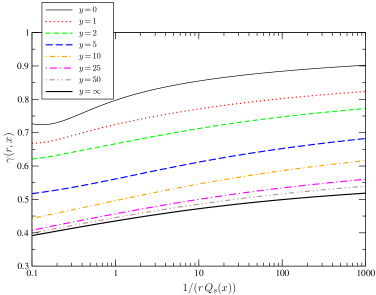
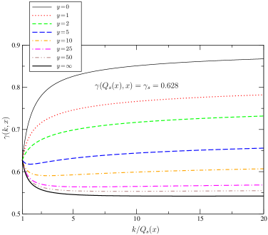
Figure 1: a) $\gamma(r,x)$ resulting from the relations (4) and (5) as a function of $1/(rQ_{s}(x))$ and $y=\log x_{0}/x$. b) $\gamma(k,x)$ as a function of $k/Q_{s}(x)$ for various rapidities $y=\log x_{0}/x$.

The resulting $\gamma(r,x)$ has the following features:

1. For $r\to 0$, $\gamma(r,x)$ asymptotically approaches 1.

2. At the saturation scale, $\gamma(r,x)$ is not a constant.

3. For decreasing $x$, $\gamma(r,x)$ approaches a limiting curve, $\gamma_{\infty}(rQ_{s}(x))$, indicated in Fig. 1 by $y=\infty$. Hence, after a longer evolution one indeed recovers geometric scaling.

The fact that for small distances $\gamma$ asymptotically approaches 1 is understandable from the BK equation, since in this limit it reduces to the BFKL equation. In the limit of small distances, the solution to the BFKL equation is dominated by either the saddle point or the initial condition, both leading to $\gamma\to 1$, since here we use the MV model as the initial condition, see [13] for details.

It turns out that $\gamma$ is clearly not constant, not even at $r=1/Q_{s}$, unlike in [8, 9, 7]. However, asymptotically geometric scaling is recovered as $\gamma$ approaches $\gamma_{\infty}$. Writing

$$\gamma(r,x)=\gamma_{\infty}(rQ_{s}(x))+\Delta\gamma(r,x)\,,$$ (6)

it turns out that, similar to the parameterizations used in [8, 9, 7], $\Delta\gamma(r,x)$ decreases as $1/y$ for $y\to\infty$ and fixed $rQ_{s}(x)$. At the saturation scale $\gamma$ is given in the small-$x$ limit by

$$\lim_{x\to 0}\gamma(r=1/Q_{s}(x),x)=\gamma_{\infty}(1)\approx 0.44\,,$$ (7)

which is significantly below $\gamma_{s}=0.628$. This is not in disagreement with theoretical expectations [6, 11]. Rather it indicates that requiring $\gamma$ in Eq. (2) to be constant at $Q_{s}$ does not follow from the BK equation.

In [8, 9, 7], $N(r,x)$ (2) was considered with $\gamma(r,x)$ replaced by $\gamma(1/k,x)$. This approximation scheme we will discuss next. The procedure of extracting $\gamma$ becomes quite different when $\gamma$ depends on $k$, since the dipole cross section $N$ then depends on both $r$ and $k$, so that it is not related to $\mathcal{N}(k,x)$ by a straightforward inverse Fourier transform (4) anymore:

$$\mathcal{N}(k,x)\equiv\int_{0}^{\infty}\frac{dr}{r}\>{J}_{0}(kr)\,\left(1-\exp\left[-\tfrac{1}{4}(r^{2}Q^{2}_{s}(x))^{\gamma(k,x)}\right]\right)\,.$$ (8)

Instead of by using the inverse Fourier transform, we will extract $\gamma$ by numerically solving Eq. (8), imposing the following condition. In order to test the Ansatz in [8, 9], we will fix $\gamma(k,x)$ in such a way that it equals the constant $\gamma_{s}\approx 0.628$ at the saturation scale. The $x$-dependence of $Q_{s}$ is determined by explicitly solving Eq. (8) for $k=Q_{s}$ and $\gamma(Q_{s},x)=0.628$. Now we can extract $\gamma$ from relation (8) for any given value of $x$ and $k$. Fig. 1 shows the results for $\gamma(k,x)$ as a function of $k/Q_{s}$ above $Q_{s}$, for a broad range of rapidities. For small rapidities the resulting $\gamma$ looks very similar to the one in [9] (cf. Fig. 4 of Ref. [9]). As one can see, for larger $y$ the resulting $\gamma$ is not compatible with the parameterization in [9] anymore; it first decreases before it rises towards 1 asymptotically.

For a discussion of additional important issues like the dependence on initial conditions, the $x$-dependence of $Q_{s}$ in our approach and the running coupling case we refer to [13].

Discussion & Conclusions

The numerical solutions of the BK equation do not display exact geometric scaling, although they approach a solution showing such scaling at asymptotic $y$. Assuming the solutions to be of the form (2), where scaling violations are encoded in the “anomalous dimension” $\gamma$, therefore leads to the conclusion that $\gamma(r,x)$ is not a function of $rQ_{s}(x)$ exclusively. In particular, it is never simply a constant, not even at the saturation scale ($r=1/Q_{s}$). At asymptotically large rapidities, $\gamma$ reaches a limiting function $\gamma_{\infty}(rQ_{s}(x))$. This function is universal for a large range of initial conditions [13]. At the saturation scale, $\gamma_{\infty}$ equals approximately $0.44$, which is considerably smaller than the corresponding values in the phenomenological models [10, 7, 9]. For small values of $rQ_{s}$ the limiting function seems to reach $\gamma_{s}$ [13], in accordance with the traveling wave results of Refs. [11].

Performing the replacement of $\gamma(r,x)\to\gamma(1/k,x)$ does allow one to find a solution for which $\gamma(k=Q_{s},x)$ is kept fixed. The behavior of $\gamma(1/k,x)$ is then for small rapidities qualitatively similar to the parameterization in [9]. However, the usually considered choice $\gamma(k=Q_{s},x)=\gamma_{s}=0.628$ yields some unwanted features, i.e. $\Delta\gamma$ being negative in a region above the saturation scale and the absence of solutions below the saturation scale, although the Ansatz was not intended for that region. Keeping $\gamma(k=Q_{s},x)$ fixed at a smaller value, e.g. at $\gamma_{\infty}(rQ_{s}=1)\approx 0.44$, seems more suitable [13], but it remains to be investigated whether such a choice allows for a good fit of all relevant DIS, $d$-$Au$ and $p$-$p$ data.

It would be interesting to consider modifications of phenomenological models for the dipole scattering amplitude that are compatible with both the BK equation and the data. Given the fact that the BK evolution does not respect geometric scaling around $Q_{s}$, phenomenological parameterizations that reflect this feature would seem a natural choice. Fortunately, the LHC and a possible future electron-ion collider will provide data over a larger range of momenta and rapidities, so that one can expect to test the evolution properties of the models more accurately.

References

-
[1]
Slides:
http://indico.cern.ch/contributionDisplay.py?contribId=69&sessionId=15&confId=9499 - [2] A. H. Mueller, Nucl. Phys. B 335, 115 (1990).
- [3] I. Balitsky, Nucl. Phys. B 463, 99 (1996); Y. V. Kovchegov, Phys. Rev. D 60, 034008 (1999).
- [4] K. Golec-Biernat and M. Wüsthoff, Phys. Rev. D 59, 014017 (1999).
- [5] A. M. Stasto, K. Golec-Biernat and J. Kwiecinski, Phys. Rev. Lett. 86, 596 (2001).
- [6] A. H. Mueller and D. N. Triantafyllopoulos, Nucl. Phys. B 640, 331 (2002).
- [7] D. Kharzeev, Y.V. Kovchegov and K. Tuchin, Phys. Lett. B 599, 23 (2004).
- [8] A. Dumitru, A. Hayashigaki and J. Jalilian-Marian, Nucl. Phys. A 765, 464 (2006).
- [9] A. Dumitru, A. Hayashigaki and J. Jalilian-Marian, Nucl. Phys. A 770, 57 (2006).
- [10] E. Iancu, K. Itakura and S. Munier, Phys. Lett. B 590, 199 (2004).
- [11] S. Munier and R. Peschanski, Phys. Rev. Lett. 91, 232001 (2003); Phys. Rev. D 69, 034008 (2004).
- [12] R. Enberg, “BKsolver: numerical solution of the Balitsky-Kovchegov nonlinear integro-differential equation”, available at URL: http://www.isv.uu.se/enberg/BK/.
- [13] D. Boer, A. Utermann and E. Wessels, Phys. Rev. D 75, 094022 (2007).