Limits of ultra-high-precision optical astrometry:
Stellar surface structures

Abstract

Aims. To investigate the astrometric effects of stellar surface structures as a practical limitation to ultra-high-precision astrometry, e.g. in the context of exoplanet searches, and to quantify the expected effects in different regions of the HR-diagram.

Methods. Stellar surface structures (spots, plages, granulation, non-radial oscillations) are likely to produce fluctuations in the integrated flux and radial velocity of the star, as well as a variation of the observed photocentre, i.e. astrometric jitter. We use theoretical considerations supported by Monte Carlo simulations (using a starspot model) to derive statistical relations between the corresponding astrometric, photometric, and radial-velocity effects. Based on these relations, the more easily observed photometric and radial-velocity variations can be used to predict the expected size of the astrometric jitter. Also the third moment of the brightness distribution, interferometrically observable as closure phase, contains information about the astrometric jitter.

Results. For most stellar types the astrometric jitter due to stellar surface structures is expected to be of order 10 micro-AU or greater. This is more than the astrometric displacement typically caused by an Earth-size exoplanet in the habitable zone, which is about 1–4 micro-AU for long-lived main-sequence stars. Only for stars with extremely low photometric variability ($<0.5$ mmag) and low magnetic activity, comparable to that of the Sun, will the astrometric jitter be of order 1 micro-AU, sufficient to allow the astrometric detection of an Earth-sized planet in the habitable zone. While stellar surface structure may thus seriously impair the astrometric detection of small exoplanets, it has in general negligible impact on the detection of large (Jupiter-size) planets and on the determination of stellar parallax and proper motion. From the starspot model we also conclude that the commonly used spot filling factor is not the most relevant parameter for quantifying the spottiness in terms of the resulting astrometric, photometric and radial-velocity variations.

1 Introduction

The accuracy of astrometric measurements has improved tremendously in the past decades as a result of new techniques being introduced, both on the ground and in space. This development will continue in the next decade, e.g Gaia is to improve parallax accuracy by another two orders of magnitude compared with Hipparcos. As a result, trigonometric distances will be obtained for the Magellanic Clouds, and thousands of Jupiter-size exoplanets are likely to be found from the astrometric wobbles of their parent stars. Even before that, ground-based interferometric techniques are expected to reach similar precisions for relative measurements within a small field. How far should we expect this trend to continue? Will nanoarcsec astrometry soon be a reality, with parallaxes measured to cosmological distances and Earth-size planets found wherever we look? Or will the accuracy ultimately be limited by other factors such as variable optical structure in the targets and weak microlensing in the Galactic halo? The aim of this project is to assess the importance of such limitations for ultra-high-precision astrometry. In this paper we consider the effects of stellar surface structures found on ordinary stars.

Future high-precision astrometric observations will in many cases be able to detect the very small shifts in stellar positions caused by surface structures. In some cases, e.g. for a rotating spotted star, the shifts are periodic and could mimic the dynamical pull of a planetary companion, or even the star’s parallax motion, if the period is close to one year. These shifts are currently of great interest as a possible limitation of the astrometric method in search for Earth-like exoplanets. We want to estimate how important these effects are for different types of stars, especially in view of current and future astrometric exoplanet searches such as VLTI-PRIMA (Reffert et al. 2005), SIM PlanetQuest (Unwin 2005) and Gaia (Lattanzi et al. 2005).

Astrometric observations determine the position of the centre of gravity of the stellar light, or what we call the photocentre. This is an integrated property of the star (the first moment of the intensity distribution across the disk), in the same sense as the total flux (the zeroth moment of the intensity distribution) or stellar spectrum (the zeroth moment as function of wavelength). In stars other than the Sun, information about surface structures usually come from integrated properties such as light curves and spectrum variations. For example, Doppler imaging (DI) has become an established technique to map the surfaces of rapidly rotating, cool stars. Unfortunately, it cannot be applied to most of the targets of interest for exoplanet searches, e.g. low-activity solar-type stars. Optical or infrared interferometric (aperture synthesis) imaging does not have this limitation, but is with current baselines ($<1$ km) in practice limited to giant stars and other extended objects (see Monnier et al. 2006 for a review on recent advances in stellar interferometry). Interferometry of marginally resolved stars may, however, provide some information about surface structures through the closure phase, which is sensitive to the third central moment (asymmetry) of the stellar intensity distribution (Monnier 2003; Lachaume 2003; Labeyrie et al. 2006).

Since there is limited information about surface structures on most types of stars, an interesting question is whether we can use more readily accessible photometric and spectroscopic data to infer something about possible astrometric effects. For example, dark or bright spots on a rotating star will in general cause periodic variations both in the integrated flux and in the radial velocity of the star, as well as in the photocentre and the asymmetry of the intensity distribution. Thus, we should at least expect the astrometric effect to be statistically related to the other effects.

We show that there are in fact relatively well-defined statistical relations between variations in the photocentre, total flux, closure phase and radial velocity for a wide range of possible surface phenomena. These relations are in the following used to predict the astrometric jitter in various types of stars, without any detailed knowledge of their actual surface structures.

2 Astrometric limits from previous studies

The discovery of exoplanets by means of high-precision radial velocity measurements has triggered an interest in how astrophysical phenomena such as magnetic activity and convective motions might affect the observed velocities (Saar et al. 2003). Evidence for dark spots have been seen photometrically and spectroscopically for many cool stars other than the Sun, and quantified in terms of an empirically determined spot filling factor$f$, ranging from $\ll 1\%$ for old, inactive stars to several percent for active stars. It is therefore natural to relate the expected radial-velocity effects to the spot filling factor. For example, Saar & Donahue (1997) used a simple model consisting of a single black equatorial spot on a rotating solar-like star to derive the following relation between $f$ (in percent), the projected rotational velocity $V\sin i$ and the amplitude $\Delta v_{r}$ of the resulting radial velocity variations:

$$\Delta v_{r}=0.0065\,f^{0.9}\,V\sin i$$ (1)

In a similar vein, Hatzes (2002) estimated both the radial velocity amplitude and the corresponding astrometric effect from a similar model, but assuming a fixed spot size ($2^{\circ}$ radius) and instead varying the number of spots placed randomly on the stellar surface centred around the equator. For the radial velocity amplitude they found

$$\Delta v_{r}=\left(0.0086\,V\sin i-0.0016\right)\,f^{0.9}$$ (2)

in approximate agreement with (1), while the total amplitude of the astrometric effect (converted to linear distance) was

$$\Delta{\rm pos}=(7.1\times 10^{-5}\leavevmode\nobreak\ \mbox{AU})\,f^{0.92}$$ (3)

Reffert et al. (2005) discuss the accuracy and limitations of the PRIMA (Phase-Referenced Imaging and Micro-Arcsecond Astrometry) facility at the VLT Interferometer in the context of the search for suitable targets for exoplanetary searches, reference and calibrations stars. According to their calculations, a spot filling factor of $f=2$% would move the photocentre of a G0V star by about $3\times 10^{-5}$ AU, roughly a factor 4 less than according to (3). They also conclude that the corresponding brightness variation is less than 2%.

But $f$ alone may not be a very good way to quantify the ‘spottiness’. For example, the photometric or astrometric effects of a large single spot are obviously very different from those of a surface scattered with many small spots, although the spot filling factor may be the same in the two cases. Therefore, more detailed (or more general) models may be required to explore the plausible ranges of the astrometric effects.

Bastian & Hefele (2005) give an assessment of the astrometric effects of starspots, and conclude that they are hard to quantify, mostly because of the insufficient statistics. Although starspots are common among cool stars with outer convective zones, data are strongly biased towards very active stars. They conclude that the effects on solar-type stars are likely to be negligible for Gaia, while much larger spots on K giants may become detectable. For supergiants and M giants, having radii of the order of $100R_{\odot}$ (or more), the effect may reach 0.25 AU (or more), which could confuse the measurement of parallax and proper motion.

Sozzetti (2005) gives an interesting review of the astrometric methods to identify and characterize extrasolar planets. As an example of the astrophysical noise sources affecting the astrometric measurements, he considers a distribution of spots on the surface of a pre-mainsequence (T Tauri) star. For a star with radius $1R_{\odot}$ seen at a distance of 140 pc, he finds that a variation of the flux in the visual by $\Delta F/F=10$% (rms) corresponds to an astrometric variation of $\sim\!3\leavevmode\nobreak\ \mu$as (rms), and that the two effects are roughly proportional.

While the astrometric effects cannot yet be tested observationally, it is possible to correlate the photometric and radial-velocity variations for some stars (Queloz et al. 2001; Henry et al. 2002). From a small sample of Hyades stars Paulson et al. (2004b) found an approximately linear relation

$$\sigma_{v_{\rm R}}\simeq 2+3600\,\sigma_{m}\quad\mbox{[m\leavevmode\nobreak\ s${}^{-1}$]}$$ (4)

between the RMS scatter in Strömgren $y$ magnitude ($\sigma_{m}$) and in radial velocity ($\sigma_{v_{\rm R}}$). This relation supports the idea that a large part of the radial-velocity scatter in these stars is caused by surface structures.

Svensson & Ludwig (2005) have computed hydrodynamical model atmospheres for a range of stellar types, predicting both the photometric and astrometric jitter caused by granulation. They find that the computed astrometric jitter is almost entirely determined by the surface gravity $g$ of the atmosphere model, and is proportional to $g^{-1}$ for a wide range of models. This relationship is explained by the increased granular cell size with increasing pressure scale height or decreasing $g$. The radius of the star does not enter the relation, except via $g$, since the increased leverage of a large stellar disk is compensated by the averaging over more granulation cells. For their most extreme model, a bright red giant with $\log g=1$ ($R/R_{\odot}\simeq 95$) they find $\sigma_{\rm pos}\simeq 300\leavevmode\nobreak\ \mu$AU. Ludwig & Beckers (2005) extended this by considering the effects of granulation on interferometric observations of red supergiants. They show that both visibilities and closure phases may carry clear signatures of deviations from circular symmetry for this type of stars, and conclude that convection-related surface structures may thus be observable using interferometry.

Ludwig (2006) outlines a statistical procedure to characterise the photometric and astrometric effects of granulation-related micro-variability in hydrodynamical simulations of convective stars. Based on statistical assumptions similar to our model in Appendix A, he finds the relation

$$\frac{\sigma_{x}}{R}\simeq\frac{1}{\sqrt{6}}\frac{\sigma_{F}}{\left\langle F\right\rangle}$$ (5)

between the RMS fluctuation of the photocentre in one coordinate ($x$), the radius of the star ($R$), and the relative fluctuations of the observed flux ($F$).

3 Modeling astrometric displacements

3.1 Relations for the astrometric jitter

In a coordinate system $\@vec{xyz}$ with origin at the centre of the star and $+\@vec{z}$ away from the observer, let $I(\@vec{r},t)$ be the instantaneous surface brightness of the star at point $\@vec{r}=(x,y,z)$ on the visible surface, i.e. the specific intensity in the direction of the observer. We are interested in the integrated properties: total flux $F(t)$, photocentre offsets $\Delta x(t)$, $\Delta y(t)$ in the directions perpendicular to the line of sight, the third central moment of the intensity distribution $\mu_{3}(t)$, and the radial velocity offset $\Delta v_{\rm R}(t)$. These are given by the following integrals over the visible surface $S$ ($z<0$):

$$F(t) = \int_{S}I(\@vec{r},t)\mu\,\mbox{d}S$$ (6)

$$\Delta x(t) = \frac{1}{F(t)}\int_{S}I(\@vec{r},t)x\mu\,\mbox{d}S$$ (7)

$$\Delta y(t) = \frac{1}{F(t)}\int_{S}I(\@vec{r},t)y\mu\,\mbox{d}S$$ (8)

$$\mu_{3}(t) = \frac{1}{F(t)}\int_{S}I(\@vec{r},t)\left[x-\Delta x(t)\right]^{3}\mu\,\mbox{d}S$$ (9)

$$\Delta v_{\rm R}(t) = \frac{1}{F(t)}\int_{S}I(\@vec{r},t)\left[(\@vec{\omega}\times\@vec{r})\cdot\hat{\@vec{z}}\right]\,\mu\,\mbox{d}S$$ (10)

where $\mu=|z|/R$ is the geometrical projection factor applied to the surface element when projected onto the sky, $\@vec{\omega}$ is the angular velocity of the star and $\hat{\@vec{z}}$ the unit vector along $+\@vec{z}$. (For the third moment, only the pure $x$ component is considered above.) Equation (10) assumes that the star rotates as a rigid body, that rotation is the only cause of the radial-velocity offset, and that the overall offset can be calculated as the intensity-weighted mean value of the local offset across the surface. The flux variation expressed in magnitudes is

$$\Delta m(t)=1.086\frac{F(t)-\left\langle F\right\rangle}{\left\langle F\right\rangle}$$ (11)

where $\left\langle F\right\rangle$ is the time-averaged flux.

Using a similar statistical method as Ludwig (2006), the RMS variations (dispersions) of $m(t)$, $\Delta x(t)$, $\Delta y(t)$ and $\mu_{3}(t)$ can be estimated from fairly general assumptions about the surface brightness fluctuations (Appendix A). This calculation is approximately valid whether the fluctuations are caused by dark or bright spots, granulation, or a combination of all three, and whether or not the time variation is caused by the rotation of the star or by the changing brightness distribution over the surface. The result is a set of proportionality relations involving the radius of the star $R$, the limb-darkening factor $a$, and the centre-to-limb variation $c$ of the surface structure contrast [see (35) and (50) for the definition of $a$ and $c$]. For $a=0.6$ (typical solar limb-darkening in visible light) and $c=0$ (no centre-to-limb variation of contrast) we find

$$\sigma_{\Delta x}=\sigma_{\Delta y}\equiv\sigma_{\mathrm{pos}} \simeq 0.376\,R\,\sigma_{m}$$ (12)

$$\sigma_{\mu_{3}} \simeq 0.139\,R^{3}\,\sigma_{m}$$ (13)

where $\sigma_{q}$ designates the dispersion of the quantity $q$.

For the radial-velocity dispersion, a similar relation can be derived under the previously mentioned conditions of a time-independent, rigidly rotating star. Using that $(\@vec{\omega}\times\@vec{r})\cdot\hat{\@vec{z}}=\omega_{x}y-\omega_{y}x$ we have

$$\Delta v_{\rm R}(t)=\omega_{x}\Delta y(t)-\omega_{y}\Delta x(t)$$ (14)

and

$$\sigma_{v_{\rm R}}^{2}=\omega_{x}^{2}\sigma_{y}^{2}+\omega_{y}^{2}\sigma_{x}^{2}=(\omega_{x}^{2}+\omega_{y}^{2})\sigma_{\rm pos}^{2}$$ (15)

since $\Delta x(t)$ and $\Delta y(t)$ are statistically uncorrelated according to Eq. (37). Noting that $R(\omega_{x}^{2}+\omega_{y}^{2})^{1/2}$ equals the projected rotational velocity $V\sin i$ we can also write (15) as

$$\sigma_{\rm pos}=R\sigma_{v_{\rm R}}/(V\sin i)$$ (16)

which may be used to predict the astrometric jitter from the radial velocity variations, if the latter are mainly caused by rotational modulation. Combined with (12) we find under the same assumption

$$\sigma_{v_{\rm R}}\simeq 0.376V\sin i\,\sigma_{m}$$ (17)

In terms of the rotation period $P=2\pi/\omega$, and assuming random orientation of $\@vec{\omega}$ in space, Eq. (16) can be written

$$\sigma_{\mathrm{pos}}=\sqrt{\frac{3}{2}}\;\frac{P}{2\pi}\,\sigma_{v_{\rm R}}\simeq 0.195\,P\,\sigma_{v_{\rm R}}$$ (18)

3.2 Modeling discrete spots

As a check of the general relations in Sect. 3.1 we have made numerical simulations with a very simple model, consisting of a limited number of (dark or bright) spots on the surface of a rotating star. The behaviour of the integrated properties are readily understood in this case (cf. Fig. 1):

• the flux is reduced in proportion to the total projected area of the visible spots (or the spot filling factor $f$);

• a black spot on, say, the $+x$ side of the star will shift the photocentre in the $-x$ direction and cause a negative skewness of the flux distribution along the $x$ direction;

• the apparent radial velocity of the star is modified, depending on whether the dark spot is located on the part of the disk moving towards the observer (giving $\Delta v_{\rm R}>0$) or away from the observer ($\Delta v_{\rm R}<0$) (Gray 2005, p. 496 and references therein).

Bright spots cause similar effects but with the opposite sign. Limb darkening of the stellar disk and a possible centre-to-limb variation of spot contrast will modify the precise amount of these shifts, but not their qualitative behaviour.

We assume a spherical star with $N$ spots that are:

• absolutely black,

• small compared to the stellar radius $R$,

• of equal area $A$ (measured as a fraction of the total surface),

• randomly spread over the whole stellar surface, and

• fixed in position on the surface, while the star rotates.

For circular spots of angular radius $\rho$ (as seen from the centre of the star), we have $A=\sin^{2}(\rho/2)$. The assumption of absolutely black spots is uncritical if we interpret $A$ as the equivalent area of the spot, i.e. the area of a completely black spot causing the same drop in flux. Bright spots can formally be handled by allowing negative $A$.

The star is assumed to rotate as a rigid body with period $P$ around an axis that is tilted an angle $i$ to the line of sight ($+z$). For the present experiments we take the $+y$ direction to coincide with the projection of the rotation vector $\@vec{\omega}$ onto the sky; thus $\omega_{x}=0$, $\omega_{y}=\omega\sin i$, and $\omega_{z}=\omega\cos i$, where $\omega=2\pi/P$. Limb darkening of the form intensity $\propto 1-a+a\mu$ is assumed, where $\mu=|z|/R$.

To model a rotating spotted star, we place the $N$ spots of the given size $A$ randomly on the surface of a spherical star and tilt the axis to a certain inclination $i$. Letting the star rotate around its axis we calculate the integrated quantities as functions of the rotational phase, taking into account the projection effect on the area of each spot (by the factor $\mu$) as well the limb-darkening law.

The effects of a single black spot as function of the rotational phase are illustrated in Fig. 1. It can be noted that the effects are not unrelated to each other; for example, the radial-velocity curve mirrors the displacement in $x$, and both of these curves look like the derivative of the photometric curve. This is not a coincidence but can be understood from fairly general relations like (14). With many spots the curves become quite complicated, but some of the basic relationships between them remain.

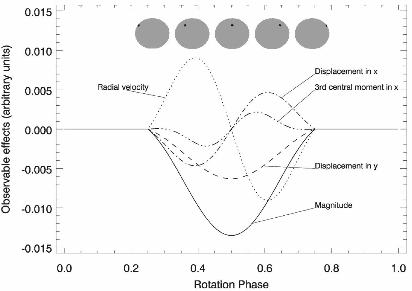
Figure 1: The curves show the effects in magnitude, position, radial velocity and intensity skewness (third central moment) of a single dark spot located at latitude $30^{\circ}$. The star is observed at inclination $i=90^{\circ}$ and the limb-darkening parameter $a=0.6$. The vertical scale is in arbitrary units for the different effects.

Figure 2: Results of Monte Carlo simulations of rotating stars with different number ($N$) of spots, all of the same size ($A=0.0025$). The different graphs refer to (from top to bottom) $\sigma_{m}$, $\sigma_{\rm pos}$, $\sigma_{\mu_{3}}$ and $\sigma_{v_{\rm R}}$, expressed on an arbitrary scale; the dots and error bars show the mean value and dispersion of the $\sigma$ values for a set of simulations with given $N$. The dashed lines have slope 0.5, corresponding to $\sigma\propto\sqrt{N}$.

The total equivalent area of the spots is $AN$ (the spot filling factor $f\simeq 2AN$). As long as $AN\ll 1$, all the effects are proportional to $A$. The dependence on $N$ is more complex because of the random distribution of spots. For example, the photometric effect will mainly depend on the actual number of spots $k$ visible at any time. For any random realization of the model, $k$ follows a binomial distribution with parameters $p=0.5$ and $N$; its dispersion is therefore $\sqrt{N}/2$. We can therefore expect the RMS photometric effect to be roughly proportional to $A\sqrt{N}$. Similar arguments (with the same result) can be made for the other effects.

Monte Carlo simulations of a large number of cases with $A=0.0025$ (spot radius $\rho=5.73^{\circ}$) and $N$ in the range from 1 to 50 (assuming random orientation of the rotation axis and a limb-darkening parameter $a=0.6$) indeed show that the RMS effects in magnitude, photocentre displacements, third central moment and radial velocity are all, in a statistical sense, proportional to $\sqrt{N}$ (Fig. 2). More precisely we find

$$\sigma_{m} \simeq (1.17\pm 0.60)\cdot A\sqrt{N}$$ (19)

$$\sigma_{\mathrm{pos}} \simeq (0.57\pm 0.25)\cdot A\sqrt{N}\cdot R$$ (20)

$$\sigma_{\mu_{3}} \simeq (0.22\pm 0.09)\cdot A\sqrt{N}\cdot R^{3}$$ (21)

$$\sigma_{v_{\rm R}} \simeq (0.51\pm 0.26)\cdot A\sqrt{N}\cdot R\,\omega$$ (22)

where the values after $\pm$ show the RMS dispersion of the proportionality factor found among the different simulations.

The relations (19)–(22) suggest that a measurement of any one of the four dispersions can be used to statistically predict the other three dispersions, assuming that we know the approximate radius and rotation period of the star, and that the different effects are indeed caused by the rotating spotted surface. An important point is that it is not necessary to know $A$ or $N$ in order to do this. For example, expressing the other effects in terms of the photometric variation we find

$$\sigma_{\rm pos} \simeq 0.49\,R\,\sigma_{m}$$ (23)

$$\sigma_{\mu_{3}} \simeq 0.19\,R^{3}\,\sigma_{m}$$ (24)

$$\sigma_{v_{\rm R}} \simeq 0.43\,R\,\omega\,\sigma_{m}$$ (25)

Comparing these relations with the theoretical results in (12)–(18) we find that the numerical factors from the numerical experiments are systematically some 30–40% larger than according to the statistical theory. This discrepancy largely vanishes if the models are constrained to high inclinations ($i\simeq\pm 90^{\circ}$). This suggests that the discrepancy is mainly caused by the small values of $\sigma_{m}$ obtained in models with small inclinations, i.e. when the star is seen nearly pole-on. The differences in these factors are in any case well within the scatter indicated in Eq. 23–25, which emphasizes the statistical nature of the predictions based e.g. on photometric variations.

It should also be noted that there is a considerable scatter between the different realisations reported in Eqs. (19)–(22), amounting to about 50% RMS about the mean RMS effect. Thus, any prediction based on either (12)–(18) or (19)–(22) is only valid in a statistical sense, with considerable uncertainty in any individual case. Nevertheless, the overall agreement between the results of these very different models suggests that the statistical relations among the different effects have a fairly general validity. The expressions for $\sigma_{v_{\rm R}}$ are the least general in this respect, as they obviously break down if the structures change on a time scale smaller than $P$, or if the surface structures themselves have velocity fields. Equations (12) and (13) do not depend on the assumption that the variability is caused by the rotation.

When modeling spotted stars, any brightening effect of faculae is often disregarded (for more details see Aarum-Ulvås 2005); only the darkening effect of spots is computed. For the Sun, the effect of faculae is known to be comparable and sometimes even larger than the darkening effect of sunspots (Eker et al. 2003; Chapman 1984; Chapman & Meyer 1986; Chapman et al. 1992; Steinegger et al. 1996). However, since the general relationships, e.g. in (12)–(18), are equally valid for bright and dark spots (or any mixture of them), it should still be possible to predict the astrometric effects from the photometric variations.

3.3 Comparison with previous studies and observations

The (near-) proportionality between the observable effects and the spot filling factor $f\propto AN$ expressed by Eqs. (1)–(3) is not supported by our spotted model, which predicts that the effects are proportional to $A\sqrt{N}$. However, for small $N$ and a filling factor of a few percent we have rough quantitative agreement with these earlier results. We note that (2) and (3) can be combined to give an approximate relation similar to (17).

Equation (5) derived by Ludwig (2006) is practically identical to our (12), which is not surprising as they are based on very similar statistical models.

Both the theoretical result and the result from the simulation for the relationship between the RMS for the radial velocity and the RMS for the magnitude shows a distinct relation and this result is confirmed by observations in the literature (Paulson et al. 2004b) for a very limited number of stars in the Hyades all having rotation period of $P\sim 8.5$ days. These are G0V–G5V stars and should therefore have approximately the same radii as the Sun ($R\sim 7\times 10^{5}$ km). Equation (25) then gives

$$\sigma_{v_{\rm R}}\simeq 2600\,\sigma_{m}\,\,[\mbox{m\leavevmode\nobreak\ s}^{-1}]$$ (26)

in reasonable agreement with the empirical result in (4). The simulations by Sozzetti (2005) give an astrometric jitter that is roughly a factor 2 greater than predicted by (12) or (23).

Thus the results of previous studies generally agree within a factor 2 or better with the theoretical formulae derived in this Section.

4 Application to real stars

In this section we use known statistics about the photometric and radial-velocity variations of real stars in order to predict the expected astrometric jitter for different types of stars. Rather than using angular units, we consistently express the astrometric jitter in linear units, using the astronomical unit AU, mAU ($10^{-3}$ AU) or $\mu$AU ($10^{-6}$ AU). This eliminates the dependence on the distance to the star, while providing simple conversion to angular units: $1\leavevmode\nobreak\ \mu$AU corresponds to $1\leavevmode\nobreak\ \mu$as at a distance of 1 pc. We also note that $1\leavevmode\nobreak\ \mbox{mAU}\simeq 0.215R_{\odot}$ and $1\leavevmode\nobreak\ \mu\mbox{AU}\simeq 150$ km.

4.1 Pre-Main Sequence (T Tauri) stars

T Tauri stars are low-mass, pre-main sequence stars in a dynamic stage of evolution often characterised by prominent dark spots, bipolar outflows or jets, accreting matter with associated rapid brightness variations, and in many cases circumstellar disks extending to a few hundred AU (e.g., Rhode et al. 2001; Herbst et al. 2002; Sicilia-Aguilar et al. 2005). Taking the star-forming region in the Orion nebula as an example, the spectral types range from G6 to M6, with the large majority in the range K0 to M4 (Rhode et al. 2001).

Many processes may contribute to the astrometric jitter of these stars besides their surface structures, e.g. photometric irregularities of the circumstellar disk. The statistical relations derived in Sect. 3 could therefore mainly set a lower limit to the likely astrometric effects. Herbst et al. (1994) found that the photometric variability of (weak) T Tauri stars (WTTS) is of the order of 0.8 mag due to cool spots and occasional flares. Assuming a typical radius of $\sim 2R_{\odot}$ (Rhode et al. 2001), Eq. (23) leads to an estimated astrometric variability of the order of $1R_{\odot}\sim 5000\leavevmode\nobreak\ \mu$AU.

4.2 Main-Sequence stars

Eyer & Grenon (1997) have used the Hipparcos photometric data to map the intrinsic variability of stars across the HR diagram. On the main sequence (luminosity class V), stars of spectral type B8–A5 and F1–F8 are among the most stable ones, with a mean intrinsic variability $\sigma_{m}<2$ mmag and with only a few percent of the stars having amplitudes above $0.05$ mag. Early B type stars are nearly all variable with a mean intrinsic variability of $\sim 10$ mmag, and among the cool stars the level and frequency of variability increases from late G to early M dwarfs. In the instability strip (A6–F0) the main-sequence stars are mostly micro-variable with $\sigma_{m}$ up to several mmag. Among F–K stars the degree of variability is probably also a strong function of age or chromospheric activity (Fekel et al. 2004); e.g., the Hyades (age $\sim 600$ Myr) show variations of about 10 mmag (Radick et al. 1995).

The Sun (G2V) is located in one of the photometrically most stable parts of the main sequence, and is one of the (as yet) few stars for which the micro-variability has been studied in detail. Analysis of the VIRGO/SoHO total solar irradiance data (Lanza et al. 2003) show variability at the level $\sigma_{m}\simeq 0.25$ mmag (relative variance $5\times 10^{-8}$) on time scales $\lesssim 30$ days, which can largely be attributed to rotational modulation. The longer-term, solar-cycle related variations are of a similar magnitude. The optical data show a strong wavelength dependence, with $\sigma_{m}\simeq 0.2$ mmag at 860 nm increasing to 0.4 mmag at 550 nm and 0.5 mmag at 400 nm (Lanza et al. 2004). For comparison, a single large sunspot group (equivalent area $A=0.05\%$, corresponding to $f=0.1\%$) gives $\sigma_{m}\simeq 0.6$ mmag according to (19).

The photometric variations of the Sun on short (rotation-related) timescales appears to be representative for solar-like stars of similar age and chromospheric activity (Fekel et al. 2004). Thus, we may expect $\sigma_{m}\lesssim 1$ mmag for ‘solar twins’ candidates, such as the sample studied by Meléndez et al. (2006). Inspection of the Hipparcos photometry for these stars (ESA 1997) confirm that most of them show no sign of variability at the sensitivity limit of a few mmag. Much more detailed and accurate statistics on micro-variability in solar-type stars are soon to be expected as a result of survey missions such as MOST (Walker et al. 2003), COROT (Baglin et al. 2002) and Kepler (Basri et al. 2005).

The increased frequency and amplitude of variations for late G-type and cooler dwarf stars is at least partly attributable to starspots. Aigrain et al. (2004) estimated stellar micro-variability as function of age and colour index from a scaling of the solar irradiance power spectrum based on the predicted chromospheric activity level. For example, they find $\sigma_{m}\simeq 1.5$ mmag in white light for old ($\sim 4.5$ Gyr) F5–K5 stars, practically independent of spectral type, while for young stars ($\sim 625$ Myr) $\sigma_{m}$ increases from 2 to 7 mmag in the same spectral range.

Variability among field M dwarfs has been studied e.g. by Rockenfeller et al. (2006), who find that a third of the stars in their sample of M2–M9 dwarfs are variable at the level of $\sigma_{m}\sim 20$ mmag. Evidence for large spots has been found for many K and M stars, yielding brightness amplitudes of up to a few tenths of a magnitude.

A large body of data on radial-velocity jitter in (mainly) F, G and K stars has been assembled from the several on-going planet search programmes and can be used to make statistical predictions as function of colour, chromospheric activity and evolutionary stage. However, since at least part of the radial-velocity jitter is caused by other effects than the rotation of an inhomogeneous surface (e.g., by atmospheric convective motions), its interpretation in terms of astrometric jitter is not straight-forward. From the observations of $\sim$450 stars in the California and Carnegie Planet Search Program, Wright (2005) finds a radial velocity jitter of $\sim\,$4 m s^-1 for inactive dwarf stars of spectral type F5 or later, increasing to some 10 m s^-1 for stars that are either active or more evolved. Saar et al. (1998), using data from the Lick planetary survey, find intrinsic radial-velocity jitters of 2–100 m s^-1 depending mainly on rotational velocity ($V\sin i$) and colour, with a minimum around $B\!-\!V\simeq 1.0$–1.3 (spectral type $\sim$K5). For a sample of Hyades F5 to M2 dwarf stars, Paulson et al. (2004a) find an average rms radial velocity jitter of $\sim$16 m s^-1.

4.3 Giant stars

For giants of luminosity class III, Hipparcos photometry has shown a considerable range in the typical degree of variability depending on the spectral type (Eyer & Grenon 1997). The most stable giants ($\sigma_{m}<2$ mmag) are the early A and late G types. The most unstable ones are of type K8 or later, with a steadily increasing variability up to $\sim\,$0.1 mag for late M giants. The stars in the instability strip (roughly from A8 to F6) are typically variable at the 5–20 mmag level. As these are presumably mainly radially pulsating, the expected astrometric jitter is not necessarily higher than on either side of the instability strip. This general picture is confirmed by other studies. Jorissen et al. (1997) found that late G and early K giants are stable at the $\sigma_{m}\leq 6$ mmag level; K3 and later types have an increasing level of micro-variability with a time scale of 5 to 10 days, while $b-y=1.1$ ($\simeq$M2) marks the onset of large-amplitude variability ($\sigma_{m}\geq 10$ mmag) typically on longer time scales ($\sim 100$ days). From a larger and somewhat more sensitive survey of G and K giants, Henry et al. (2000) found the smallest fraction of variables in the G6–K1 range, although even here some 20% show micro-variability at the 2–5 mmag level; giants later than K4 are all variable, half of them with $\sigma_{m}\geq 10$ mmag. The onset of large-amplitude variability coincides with the coronal dividing line (Haisch et al. 1991) separating the earlier giants with a hot corona from the later types with cool stellar winds. This suggests that the variability mechanisms may be different on either side of the dividing line, with rotational modulation of active regions producing the micro-variability seen in many giants earlier than K3 and pulsation being the main mechanism for the larger-amplitude variations in the later spectral types (Henry et al. 2000).

Several radial-velocity surveys of giants (Frink et al. 2001; Setiawan et al. 2004; Hekker et al. 2006) show increasing intrinsic radial-velocity variability with $B\!-\!V=1.2$, with a more or less abrupt change around $B\!-\!V=1.2$ ($\simeq\,$K3). Most bluer giants have $\sigma_{v_{\rm R}}\simeq 20$ m s^-1 while the redder ones often have variations of 40–100 m s^-1.

4.4 Bright giants and supergiants

With increasing luminosity, variability becomes increasingly common among the bright giants and supergiants (luminosity class II–Ia). The Hipparcos survey (Eyer & Grenon 1997) shows a typical intrinsic scatter of at least 10 mmag at most spectral types, and of course much more in the instability strip (including the cepheids) and among the red supergiants (including semiregular and irregular variables). Nevertheless there may be a few ‘islands’ in the upper part of the observational HR diagram where stable stars are to be found, in particular around G8II.

It is clear that pulsation is a dominating variability mechanism for many of these objects. However, ‘hotspots’ and other deviations from circular symmetry has been observed in interferometrical images of the surfaces of M supergiants and Mira varibles (e.g., Tuthill et al. 1997, 1999), possibly being the visible manifestations of very large convection cells, pulsation-induced shock waves, patchy circumstellar extinction, or some other mechanism. Whatever the explanation for these asymmetries may be, it is likely to produce both photometric and astrometric variations, probably on time scales of months to years. Kiss et al. (2006) find evidence of a strong $1/f$ noise component in the power spectra of nearly all red supergiant semiregular and irregular variable stars in their sample, consistent with the picture of irregular variability caused by large convection cells analogous to the granulation-induced variability background seen for the Sun.

4.5 Summary of expected astrometric jitter

Table 1 summarises much of the data discussed in this Section for the main-sequence, giant and supergiant stars, and gives the corresponding estimates of the astrometric jitter ($\sigma_{\rm pos}$) based on theoretical formulae. These estimates are given in three columns labelled with the corresponding equation number:

• Equation (12) is used to predict the positional jitter from the typical values of photometric variability in column $\sigma_{m}$. This is based on the assumption that the variability is due either to (dark or bright) spots, granulation, or any other surface features that vary with time. Note that the temporal variation need not be related to stellar rotation. The resulting $\sigma_{\rm pos}$ are probably realistic order-of-magnitude estimates except when the photometric variability is mainly caused by radial pulsations. In such cases (e.g., for stars in the instability strip and red supergiants) the values given clearly represent upper limits to the real effect.

• Equation (18) is used to predict the astrometric effect from the radial-velocity variability in column $\sigma_{v_{\rm R}}$. This is only valid if the radial velocity is rotationally modulated. Since pulsations, non-radial oscillations, convection and many other effects may cause radial-velocity variations without a corresponding astrometric effect, these estimates are again upper limits. Nevertheless, rotational modulation is important among active (young) main-sequence stars and M dwarfs, and for these objects Eq. (18) may provide correct order-of-magnitude estimates.

• Finally we have included an estimate of the astrometric jitter based on the following equation

  $$\sigma_{\rm pos}=(300\leavevmode\nobreak\ \mu\mbox{AU})\times 10^{1-\log g}$$ (27)

  with $\log g$ taken from Cox (2000). Equation (27) is derived from the inverse relation to surface gravity $g$ found by Svensson & Ludwig (2005) for a range of hydrodynamical model atmospheres. Although the authors warn that sphericity effects may render an extrapolation of this relation to supergiants very uncertain, we have applied it to all the stellar types in the table. Since it only includes the random effects of stellar granulation, it represents a lower limit to the expected astrometric jitter.

If the estimates based on the photometric and radial-velocity estimates are strictly considered as upper limits, the results in the table appear rather inconclusive. However, if the likely mechanisms of the variabilities are also considered, it is possible to make some quantitative conclusions. For main-sequence A to M stars, the expected level of astrometric jitter is generally in the range 2–20 $\mu$AU probably depending mainly on the level of stellar activity; old, inactive stars should have less jitter (2–5 $\mu$AU). The Sun appears to be more stable than the typical old, solar-like star, but not by a large factor. The most stable giant stars are the late F to early K types, were the expected astrometric jitter is of order 25 $\mu$AU. Late-type giants and supergiants have $\sigma_{\rm pos}$ of a hundred to several thousand $\mu$AU.

Table 1: A summary of typical photometric and spectroscopic variability for different stellar types, and inferred levels of astrometric jitter ($\sigma_{\rm pos}$). The jitter is estimated in three different ways: from the photometric variability, using Eq. (12) [this will overestimate the jitter if part of the variability is due to radial pulsation]; from the radial-velocity variability, using Eq. (18) [this method will overestimate the jitter if the variability is not caused by rotational modulation]; and from the surface gravity, using Eq. (27) [this only includes jitter caused by granulation, and is therefore a lower limit]. References to typical observed quantities are given as footnotes. Radii and $\log g$ (not shown) are taken from Cox (2000).

Type		$\sigma_{m}$	$\sigma_{v_{\rm R}}$	$R$	$P$	$\sigma_{\rm pos}$ (12)	$\sigma_{\rm pos}$ (18)	$\sigma_{\rm pos}$ (27)
		[mmag]	[m s-1]	[$R_{\odot}$]	[d]	[$\mu$AU]	[$\mu$AU]	[$\mu$AU]
Main sequence stars:
	O–B7V	10c		7		120		0.3
	B8–A5V	$<$2c		2.5		$<$9		0.2
	A6–F0V	2–8c		1.6		5–20		0.1
	F1–F8V	$<$2c	3–100m	1.3	3b	$<$5	1–30	0.1
	F9–K5V (young)	5–15a,d,k	16j	1	10a	10–25	18	0.1
	F9–K5V (old)	1–3a,d	3–5k	1	25a	2–5	8–14	0.1
	G2V (Sun)	0.4i		1	25b	0.7		0.1
	K6–M1V	10c	5m	0.6	40a	10	20	0.1
	M2–M9V	20l	10m	0.3	0.2–2l	10	0.2–2	0.04
Giants:
	O–B7III	4–8c		10		70–140		1
	B8–A7III	$<$4c		5		$<$35		1.5
	A8–F6III	5–20c		5		50–200		2
	F7–G5III	2–6c	$<$20f	7	10b	25–75	$<$25	5
	G6–K2III	$<$2c,g	20–30e,f,n	15	30b	$<$50	60	20
	K3–K8III	5–10c,h	20–100e,f,n	25		200–500		50
	M0III	20c,h	30–150e,f,n	40		1400		150
	M5III	100c,h	50–300e,f,n	90		16000
Bright giants and supergiants:
	O–AIa,b	4–40c		30		200–2000		25
	FIa,b	20–100d		100		4000–20 000		100
	GII	2–10c		30		100–500		40
	G–KIa,b	10–100c		150		3000–30 000		250
	MIa,b,II	$\sim$100c		500		$\sim$100 000		300–3000
References: aAigrain et al. (2004), bCox (2000), cEyer & Grenon (1997), dFekel et al. (2004), eFrink et al. (2001), fHekker et al. (2006), gHenry et al. (2002), hJorissen et al. (1997), iLanza et al. (2004), jPaulson et al. (2004b), kRadick et al. (1995), lRockenfeller et al. (2006), mSaar et al. (1998), nSetiawan et al. (2004)

5 Discussion

5.1 Astrometric signature of exoplanets

The possibility for an astrometric detection of a planet depends on the angular size of the star’s wobble on the sky relative to the total noise of the measurements, including the astrophysically induced astrometric jitter discussed in the previous section. In linear measure, the size of the wobble is approximately given by the semi-major axis of the star’s motion about the common centre of mass, or the astrometric signature

$$\alpha=\frac{M_{\rm p}}{M_{\ast}+M_{\rm p}}\,a\simeq\frac{M_{\rm p}}{M_{\ast}}\,a$$ (28)

(cf. Lattanzi et al. 2000, who however express this as an angle), where $M_{\rm p}$ is the mass of the exoplanet, $M_{\ast}$ that of the star, and $a$ the semi-major axis of the relative orbit. In all cases of interest here, $M_{\rm p}\ll M_{\ast}$, so that the second equality can be used.

It is of interest to evaluate the astrometric signature for the already detected exoplanets. For most of them we only know $M_{\rm p}\sin i$ from the radial-velocity curve, and we use this as a proxy for $M_{\rm p}$. This somewhat underestimates the astrometric effect, but not by a large factor since the spectroscopic detection method is strongly biased against systems with small $\sin i$. Analysing the current (April 2007) data in the Extrasolar Planets Encyclopaedia (Schneider 2007) we find a median value $\alpha\simeq 1200\leavevmode\nobreak\ \mu$AU; the 10th and 90th percentiles are 15 and 10 000 $\mu$AU.

Future exoplanet searches using high-precision astrometric techniques may however primarily target planets with masses in the range from 1 to 10 Earth masses ($M_{\rm Earth}\simeq 3\times 10^{-6}M_{\odot}$) in the habitable zone of reasonably long-lived main-sequence stars (spectral type A5 and later, lifetime $\la 1$ Gyr). For a star of luminosity $L$ we may take the mean distance of the habitable zone to be $a\sim(L/L_{\odot})^{1/2}$ AU (Kasting et al. 1993; Gould et al. 2003). In this mass range ($\sim 0.2$–$2\leavevmode\nobreak\ M_{\odot}$) the luminosity scales as $M_{\ast}^{4.5}$ (based on data from Andersen 1991), so we find $a\propto M_{\ast}^{2.25}$ and

$$\alpha\simeq\left(3\leavevmode\nobreak\ \mu\mbox{AU}\right)\times\left(\frac{M_{\rm p}}{M_{\rm Earth}}\right)\left(\frac{M_{\ast}}{M_{\odot}}\right)^{1.25}$$ (29)

For a planet of one Earth mass orbiting a main-sequence star, this quantity ranges from about 7 $\mu$AU for an A5V star to 2.3 $\mu$AU for spectral type K0V.

Lopez et al. (2005) have argued that life will have time to develop also in the environments of subgiant and giant stars, during their slow phases of development. The habitable zone may extend out to 22 AU for a 1 $M_{\odot}$ star, with a correspondingly larger astrometric signature. However, the long period of such planets would make their detection difficult for other reasons.

5.2 Exoplanet detection

The detection probability is in reality a complicated function of many factors such as the number of observations, their temporal distribution, the period and eccentricity of the orbit, and the adopted detection threshold (or probability of false detection). A very simplistic assumption might be that detection is only possible if the RMS perturbation from the planet exceeds the RMS noise from other causes. Neglecting orbital eccentricity and assuming that the orbital plane is randomly oriented in space, so that $\langle\sin^{2}i\rangle=2/3$, the RMS positional excursion of the star in a given direction on the sky is $\alpha/\sqrt{3}$. With a sufficiently powerful instrument, so that other error sources can be neglected, the condition for detection then becomes $\alpha/\sigma_{\rm pos}\ga\sqrt{3}$. In reality, a somewhat larger ratio than $\sqrt{3}$ is probably required for a reliable detection, especially if the period is unknown. For example, Sozzetti (2005) reports numerical simulations showing that $\alpha/\sigma\ga 2$ is required for detection of planetary signatures by SIM or Gaia, where $\sigma$ is the single-epoch measurement error, provided that the orbital period is less than the mission length. (For the corresponding problem of detecting a periodic signal in radial-velocity data, Marcy et al. (2005) note that a velocity precision of 3 m s^-1 limits the detected velocity semi-amplitudes to greater than $\sim$10 m s^-1, implying an even higher amplitude/noise ratio of 3.3.) As a rule-of-thumb, we assume that detection by the astrometric method is at least in principle possible if

$$\sigma_{\rm pos}\la 0.5\alpha$$ (30)

For old, solar-type stars the expected astrometric jitter is $\la$5 $\mu$AU, implying that exoplanets around these stars with $\alpha\ga 10\leavevmode\nobreak\ \mu$AU could generally be detected and measured astrometrically. This applies to the vast majority ($>$90%) of the exoplanets already detected by the radial-velocity method. Such observations would be highly interesting for obtaining independent information about these systems, in particular orbital inclinations and unambiguous determination of planetary masses.

Exoplanets of about 10 $M_{\rm Earth}$ orbiting old F–K main-sequence stars in the habitable zone ($\alpha\simeq 20$–50 $\mu$AU) would generally be astrometrically detectable. This would also be the case for Earth-sized planets in similar environments ($\alpha\simeq 2$–5 $\mu$AU), but only around stars that are unusually stable, such as the Sun.

5.3 Determination of parallax and proper motion

The primary objective of high-precision astrometric measurements, apart from exoplanet detection, is the determination of stellar parallax and proper motion. We consider here only briefly the possible effects of stellar surface structures on the determination of these quantities.

Stellar parallax causes an apparent motion of the star, known as the parallax ellipse, which is an inverted image the Earth’s orbit as viewed from the star. The linear amplitude of the parallax effect is therefore very close to 1 AU. (For a space observatory at the Sun–Earth Lagrangian point L₂, such as Gaia, the mean amplitude is 1.01 AU.) Thus, the size of the astrometric jitter expressed in AU can directly be used to estimate the minimum achievable relative error in parallax. For main-sequence stars this relative error is less than $10^{-4}$, for giant stars it is of order $10^{-4}$ to $10^{-3}$, and for supergiants it may in some cases exceed 1%. We note that a 1% relative error in parallax gives a 2% (0.02 mag) error in luminosity or absolute magnitude.

If proper motions are calculated from positional data separated by $T$ years, the random error caused by the astrometric jitter, converted to transverse velocity, is $\simeq\sigma_{\rm pos}\sqrt{2}/T$. Even for a very short temporal baseline such as $T=1$ yr, this error is usually very small: $\sim$0.1 m s^-1 for main-sequence stars and $\sim$0.5–5 m s^-1 for giants. (Note that $1\leavevmode\nobreak\ \mbox{AU\leavevmode\nobreak\ yr}^{-1}\simeq 4.74\leavevmode\nobreak\ \mbox{km\leavevmode\nobreak\ s}^{-1}$.) In most applications of stellar proper motions this is completely negligible.

6 Conclusions

For most instruments on ground or in space, stars are still unresolved or marginally resolved objects that can only be observed by their disk-integrated properties. The total flux, astrometric position, effective radial velocity and closure phase are examples of such integrated properties. Stellar surface structures influence all of them in different ways. Our main conclusions are:

1. Theoretical considerations allow to establish statistical relations between the different integrated properties of stars. Under certain assumptions these relations can be used to predict the astrometric jitter from observed variations in photometry, radial velocity or closure phase.

2. The total flux, astrometric position and third central moments (related to closure phase) are simple moments of the intensity distribution over the disk, and for these the statistical relations are valid under fairly general conditions – for example, they hold irrespective of whether the variations are caused by spots on a rotating star or by the temporal evolution of granulation. By contrast, radial-velocity variations can only be coupled to photometric and astrometric variations if they are primarily caused by rotational modulation.

3. The theoretical relations are supported by numerical simulations using a model of a rotating spotted star. In this case the variations in total flux, position, radial velocity and closure phase are all proportional to $A\sqrt{N}$, where $A$ is the equivalent area of each spot and $N$ the number of spots. This means that, e.g., the astrometric jitter can be (statistically) predicted from the photometric variability without knowing $A$ and $N$. It is noted that the spot filling factor, being proportional to $AN$, is not the most relevant characteristic of spottiness for these effects.

4. Using typical values for the observed photometric and radial-velocity variations in ordinary stars, we have estimated the expected size of the astrometric jitter caused by surface structures (Table 1). The estimates range from below 1 $\mu$AU for the Sun, several $\mu$AU for most main-sequence stars, some tens of $\mu$AU for giants, and up to several mAU for some supergiants.

5. The expected positional jitter has implications for the possible astrometric detection of exoplanets. While planets heavier than 10 Earth masses may be astrometrically detected in the habitable zone around ordinary main-sequence stars, it is likely that Earth-sized planets can only be detected around stars that are unusually stable for their type, similar to our Sun.

6. Stellar surface structures in general have negligible impact on other astrometric applications, such as the determination of parallax and proper motion. A possible exception are supergiants, where very large and slowly varying spots or convection cells could limit the relative accuracy of parallax determinations to a few per cent.

Appendix A Statistical properties of the spatial moments of the intensity distribution across a stellar disk

In this Appendix we derive the mean values and variances of the moments $\langle x^{m}y^{n}\rangle$ for a spherical star, where $x$ and $y$ are spatial coordinates normal to the line-of-sight and $\langle\rangle$ denotes the instantaneous flux-weighted mean. The analysis extends and generalizes that of Ludwig (2006) by considering also the third moment (relevant for measurement of closure phase) and a centre-to-limb variation of the intensity contrast.

Let $\theta,\varphi$ be polar coordinates on the stellar surface with $\theta=0$ at the centre of the visible disk and $\varphi=0$ along the $x$ axis. With $\mu=\cos\theta$ we write the instantaneous intensity across the visible stellar surface $S$ as $I(\mu,\varphi)$, and introduce the non-normalized spatial moments

$$M_{mn}\equiv\int_{S}\mbox{d}S\,I(\mu,\varphi)\,\mu\,x^{m}\,y^{n}=$$ (31)

$$R^{m+n+2}\!\!\int_{0}^{1}\!\!\mbox{d}\mu\!\int_{0}^{2\pi}\!\!\!\mbox{d}\varphi\,I(\mu,\varphi)\,\mu\,(1-\mu^{2})^{(m+n)/2}\cos^{m}\!\varphi\,\sin^{n}\!\varphi$$

where $x=R\,(1-\mu^{2})^{1/2}\cos\varphi$ and $y=R\,(1-\mu^{2})^{1/2}\sin\varphi$. The factor $\mu$ in the integrand is the foreshortening of the surface element $\mbox{d}S=R^{2}\mbox{d}\mu\,\mbox{d}\varphi$ when projected normal to the line-of-sight. The normalized moments are given by

$$\langle x^{m}y^{n}\rangle=\frac{M_{mn}}{M_{00}}$$ (32)

where it can be noted that $M_{00}$ equals the instantaneous total stellar flux.

It is assumed that $I(\mu,\varphi)$ varies randomly both across the stellar surface (at a given instant), and as a function of time. As a consequence, the spatial moments (31) and (32) are also random functions of time, and the goal is to characterize them in terms of their mean values and variances. Since we are interested in quite small effects of the surface structure it is generally true that the dispersions are small compared with the total flux and scale of the star, so that for example $\mbox{D}[M_{00}]\ll\mbox{E}[M_{00}]$ and $\mbox{D}[M_{10}]\ll R\,\mbox{E}[M_{00}]$. In this case the variability of $\langle x^{m}y^{n}\rangle$ is mainly produced by the numerator in (32), and we may use the approximations

$$\mbox{E}[\langle x^{m}y^{n}\rangle]=\frac{\mbox{E}[M_{mn}]}{\mbox{E}[M_{00}]}\,,\quad\mbox{D}[\langle x^{m}y^{n}\rangle]=\frac{\mbox{D}[M_{mn}]}{\mbox{E}[M_{00}]}$$ (33)

In the following we therefore focus on deriving the mean values and dispersions of the non-normalized moments $M_{mn}$. The (temporal) mean value and dispersion of $I(\mu,\varphi)$ are assumed to be independent of $\varphi$; thus

$$\mbox{E}[I(\mu,\varphi)]=A(\mu)\,,\quad\mbox{D}[I(\mu,\varphi)]=\sigma_{I}(\mu)$$ (34)

where $A(\mu)$ and $\sigma_{I}(\mu)$ are functions to be specified.

A.1 Mean value of the moments

We assume a linear limb-darkening law with coefficient $a$, such that

$$A(\mu)=(1-a+a\mu)A_{1}$$ (35)

where $A_{1}$ is the mean intensity at the disk centre ($\mu=1$). From (31) we obtain

$$\mbox{E}[M_{mn}]=$$ (36)

$$R^{m+n+2}\!\!\int_{0}^{1}\!\!\mbox{d}\mu\!\int_{0}^{2\pi}\!\!\!\mbox{d}\varphi\,A(\mu)\,\mu\,(1-\mu^{2})^{(m+n)/2}\cos^{m}\!\varphi\,\sin^{n}\!\varphi$$

which with (35) evaluates to

$$\mbox{E}[M_{mn}]=0$$ (37)

if either $m$ or $n$ is odd, and to

$$\mbox{E}[M_{mn}]=2\pi R^{m+n+2}\,\frac{(m-1)!!(n-1)!!}{(m+n)!!}\,A_{1}H_{m+n}(a)$$ (38)

if both $m$ and $n$ are even. Here, we introduced the functions

$$H_{k}(a) = \int_{0}^{1}\!\!\mbox{d}\mu\,(1-a+a\mu)\,\mu\,(1-\mu^{2})^{k/2}$$ (41)

$$= \left\{\begin{array}[]{lll}{\displaystyle\frac{1-a}{k+2}+\frac{k!!}{(k+3)!!}\,a}&&\mbox{(even\leavevmode\nobreak\ $k$)}\\[12.0pt] {\displaystyle\frac{1-a}{k+2}+\frac{k!!}{(k+3)!!}\,\frac{\pi}{2}\,a}&&\mbox{(odd\leavevmode\nobreak\ $k$)}\end{array}\right.$$

of which, presently, we only need

$$H_{0}(a)=\frac{1}{2}-\frac{a}{6}\qquad\mbox{and}\qquad H_{2}(a)=\frac{1}{4}-\frac{7a}{60}$$ (42)

Thus, the mean total flux is

$$\mbox{E}[M_{00}]=\pi R^{2}\,A_{1}\,\left(1-\frac{a}{3}\right)$$ (43)

and the second moments

$$\mbox{E}[M_{20}]=\mbox{E}[M_{02}]=\frac{1}{4}\,\pi R^{4}\,A_{1}\,\left(1-\frac{7a}{15}\right)$$ (44)

The rms extension of the star in either coordinate is given by

$$s=\left(\frac{\mbox{E}[M_{20}]}{\mbox{E}[M_{00}]}\right)^{1/2}=\left(\frac{\mbox{E}[M_{02}]}{\mbox{E}[M_{00}]}\right)^{1/2}=\frac{R}{2}\,\left(\frac{1-7a/15}{1-a/3}\right)^{1/2}$$ (45)

A.2 Dispersion of the moments

In order to compute the dispersion of $M_{mn}$ we need to introduce the second-order statistics of $I(\mu,\varphi)$. Following Ludwig (2006) we divide the visible hemisphere into $N$ equal surface patches of size $\Delta A=R^{2}\Delta\theta\Delta\varphi\sin\theta=R^{2}\Delta\mu\Delta\varphi=2\pi R^{2}/N$, with the centre of patch $k$ at position $(\mu_{k},\varphi_{k})$. Thus the integral over the visible surface of any function $g(\mu,\varphi)$ can in the limit of large $N$ be replaced by a sum:

$$R^{2}\!\!\int_{0}^{1}\!\!\mbox{d}\mu\!\int_{0}^{2\pi}\!\!\!\mbox{d}\varphi\,g(\mu,\varphi)\simeq\frac{2\pi R^{2}}{N}\sum_{k=1}^{N}g(\mu_{k},\varphi_{k})$$ (46)

In particular, from (31) we have

$$M_{mn}=\frac{2\pi R^{m+n+2}}{N}\sum_{k=1}^{N}I_{k}\,\mu_{k}\,(1-\mu_{k}^{2})^{(m+n)/2}\cos^{m}\!\varphi_{k}\,\sin^{n}\!\varphi_{k}$$ (47)

where $I_{k}$ is the mean value of $I(\mu,\varphi)$ in patch $k$. This expresses the moment as a linear combination of the random variables $I_{k}$. If we now assume that the intensity variations $\Delta I_{k}=I_{k}-\mbox{E}[I_{k}]$ of the patches are uncorrelated, i.e. $\mbox{E}[\Delta I_{k}\Delta I_{k^{\prime}}]=0$ for $k\neq k^{\prime}$, we have

$$\mbox{V}[M_{mn}]=$$ (48)

$$\frac{4\pi^{2}R^{2m+2n+4}}{N^{2}}\sum_{k=1}^{N}\mbox{V}[I_{k}]\,\mu_{k}^{2}\,(1-\mu_{k}^{2})^{m+n}\cos^{2m}\!\varphi_{k}\,\sin^{2n}\!\varphi_{k}$$

For sufficiently large $N$ the patches would resolve even the smallest surface structures and we would have $\mbox{V}[I_{k}]=\sigma_{I}^{2}(\mu_{k})$ according to (34). However, in that case the intensities of adjacent patches would be correlated, so (48) would not hold. For the latter equation we effectively need patches that are larger than the correlation length of the surface structures. We must therefore assume that $N$ is large enough for the discretization (44) to hold, and still small enough that the patches are uncorrelated. In this regime we have $\mbox{V}[I_{k}]<\sigma_{I}^{2}(\mu_{k})$, since $I_{k}$ is the average intensity in patch $k$, not the local intensity at point $(\mu_{k},\varphi_{k})$. In fact, $\mbox{V}[I_{k}]$ will depend on the patch size (or $N$) in such a way that $\mbox{V}[I_{k}]/N$ is invariant (Ludwig 2006). (This is obviously the case for independent patches: grouping them into larger and fewer patches decreases the variance in proportion to the resulting $N$.) We write the invariant quantity as

$$\frac{\mbox{V}[I_{k}]}{N}=A(\mu_{k})^{2}C(\mu_{k})^{2}$$ (49)

where $A(\mu)$ is the mean intensity as before and $C(\mu)$ the centre-to-limb variation of the contrast (scaled by $N^{-1/2}$). In analogy with (35) we assume a linear centre-to-limb variation of the contrast according to

$$C(\mu)=(1-c+c\mu)C_{1}$$ (50)

Inserting (49) and (50) into (48) and using (46) to transform the sum into an integral gives

$$\mbox{V}[M_{mn}]=2\pi R^{2m+2n+4}\times$$ (51)

$$\times\int_{0}^{1}\!\!\mbox{d}\mu\!\int_{0}^{2\pi}\!\!\!\mbox{d}\varphi\,A(\mu)^{2}C(\mu)^{2}\,\mu^{2}\,(1-\mu^{2})^{m+n}\cos^{2m}\!\varphi\,\sin^{2n}\!\varphi$$

$$= 4\pi^{2}R^{2m+2n+4}\,\frac{(2m-1)!!(2n-1)!!}{(2m+2n)!!}\,A_{1}^{2}C_{1}^{2}\,K_{m+n}(a,c)$$

where we introduced the functions

$$K_{k}(a,c)=\int_{0}^{1}\!\!\mbox{d}\mu\,(1-a+a\mu)^{2}(1-c+c\mu)^{2}\mu^{2}(1-\mu^{2})^{k}$$ (52)

For $k=0,\dots 3$ we have

$$K_{0}(a,c) = \frac{1}{3}-\frac{1}{6}\,(a+c)+\frac{1}{30}\,(a^{2}+4ac+c^{2})$$ (53)

$$\qquad-\frac{1}{30}\,ac(a+c)+\frac{1}{105}\,a^{2}c^{2}$$

$$K_{1}(a,c) = \frac{2}{15}-\frac{1}{10}\,(a+c)+\frac{1}{42}\,(a^{2}+4ac+c^{2})$$ (54)

$$\qquad-\frac{11}{420}\,ac(a+c)+\frac{1}{126}\,a^{2}c^{2}$$

$$K_{2}(a,c) = \frac{8}{105}-\frac{29}{420}\,(a+c)+\frac{23}{1260}\,(a^{2}+4ac+c^{2})$$ (55)

$$\qquad-\frac{3}{140}\,ac(a+c)+\frac{47}{6930}\,a^{2}c^{2}$$

$$K_{3}(a,c) = \frac{16}{315}-\frac{13}{252}\,(a+c)+\frac{29}{1980}\,(a^{2}+4ac+c^{2})$$ (56)

$$\qquad-\frac{25}{1386}\,ac(a+c)+\frac{38}{6435}\,a^{2}c^{2}$$

Using (33) we obtain the following general expression for the dispersion of the normalized spatial moment $D_{mn}\equiv\mbox{D}[\langle x^{m}y^{n}\rangle]$:

$$D_{mn}=C_{1}\,R^{m+n}\,\frac{\sqrt{\displaystyle\frac{(2m-1)!!^{\phantom{{}^{\prime}}}(2n-1)!!}{(2m+2n)!!}\,K_{m+n}(a,c)}}{H_{0}(a)}$$ (57)

Note that $D_{00}=\mbox{D}[M_{00}]/\mbox{E}[M_{00}]$ is the relative dispersion of the total flux, $D_{10}$ is the dispersion of the photocentre along the $x$ axis, etc. We have in particular

$$D_{00} = C_{1}\,\frac{\sqrt{\!{}^{\phantom{{}^{\prime}}}K_{0}(a,c)}}{H_{0}(a)}$$ (58)

$$D_{10} = D_{01}=C_{1}\,R\,\frac{\sqrt{\frac{1}{2}K_{1}(a,c)}}{H_{0}(a)}$$ (59)

$$D_{20} = D_{02}=C_{1}\,R^{2}\,\frac{\sqrt{\frac{3}{8}K_{2}(a,c)}}{H_{0}(a)}$$ (60)

$$D_{30} = D_{03}=C_{1}\,R^{3}\,\frac{\sqrt{\frac{5}{16}K_{3}(a,c)}}{H_{0}(a)}$$ (61)

A.3 The third central moment

Closure phase is sensitive to the asymmetry of the stellar image, and the third moments ($M_{mn}$ for $m+n=3$) are intended to provide a statistical characterization of this asymmetry. These moments are calculated with respect to the geometrical centre of the disk (at $x=y=0$). However, intrinsic image properties such as size, shape and asymmetry are more properly expressed with respect to the photocentre, at $x_{0}=M_{10}/M_{00}$, $y_{0}=M_{01}/M_{00}$, i.e., by means of central moments (here denoted with a prime). For example, the third central moment along the $x$ axis is given by

$$M_{30}^{\prime}=\int_{S}\mbox{d}S\,I(\mu,\varphi)\,\mu\,(x-x_{0})^{3}$$ (62)

$$\quad=M_{30}-3x_{0}M_{20}+3x_{0}^{2}M_{10}-x_{0}^{3}M_{00}$$

$$\quad=M_{30}-3\,\frac{M_{10}M_{20}}{M_{00}}+2\,\frac{M_{10}^{3}}{M_{00}^{2}}$$

It is seen that $\mbox{E}[M_{30}^{\prime}]=0$ as expected. However, to calculate the variance of $M_{30}^{\prime}$ it is necessary to make some approximations. First we replace the even moments in the right-hand side of (58) by their mean values and introduce the rms extent $s$ of the stellar disk from (45), yielding

$$M_{30}^{\prime}=M_{30}-3M_{10}\left(s^{2}-\frac{2}{3}\,x_{0}^{2}\right)$$ (63)

The photocentre displacement is normally very small compared with the size of the disk, so that the second term in the parentheses can be neglected. Then

$$\mbox{V}[M_{30}^{\prime}]=\mbox{E}[M_{30}^{\prime 2}]=\mbox{E}[M_{30}^{2}]-6s^{2}\mbox{E}[M_{10}M_{30}]+9s^{4}\mbox{E}[M_{10}^{2}]$$ (64)

$$\quad=\mbox{V}[M_{30}]-6s^{2}\mbox{V}[M_{20}]+9s^{4}\mbox{V}[M_{10}]$$

using that $\mbox{E}[M_{10}M_{30}]=\mbox{V}[M_{20}]$. Finally, the dispersion of the normalized third central moment is found to be

$$D_{30}^{\prime} = \frac{C_{1}R^{3}}{H_{0}(a)}\left\lgroup\displaystyle\frac{5}{16}\,K_{3}(a,c)-\frac{9}{8}\,\frac{H_{2}(a)}{H_{0}(a)}\,K_{2}(a,c)+\phantom{\left(\frac{H_{2}(a)}{H_{0}(a)}\right)^{2}}\right.$$ (65)

$$\left.\qquad\qquad{}+\frac{9}{8}\,\left(\frac{H_{2}(a)}{H_{0}(a)}\right)^{2}K_{1}(a,c)\right\rgroup^{1/2}$$

A.4 Scaling relations

Since all the dispersions in (58) and (65) are proportional to $C_{1}$ we obtain a set of simple scaling relations that can be used to predict the dispersion of a certain moment from a measurement of the dispersion of a different moment (assuming that $a$ and $c$ are approximately known). The most useful relations allow to predict the dispersions of the first and third moments from that of the total flux (zeroth moment). For the first moment (photocentre) we have

$$\frac{\mbox{D}[M_{10}]}{\mbox{D}[M_{00}]}=R\left\lgroup\frac{K_{1}(a,c)}{2K_{0}(a,c)}\right\rgroup^{1/2}$$ (66)

and for the third central moment

$$\frac{\mbox{D}[M_{30}^{\prime}]}{\mbox{D}[M_{00}]}=R^{3}\left\lgroup\displaystyle\frac{5}{16}\,\frac{K_{3}(a,c)}{K_{0}(a,c)}-\frac{9}{8}\,\frac{H_{2}(a)}{H_{0}(a)}\,\frac{K_{2}(a,c)}{K_{0}(a,c)}+\phantom{\left(\frac{H_{2}(a)}{H_{0}(a)}\right)^{2}}\right.$$ (67)

$${}\left.\qquad\qquad\qquad{}+\frac{9}{8}\,\left(\frac{H_{2}(a)}{H_{0}(a)}\right)^{2}\frac{K_{1}(a,c)}{K_{0}(a,c)}\right\rgroup^{1/2}$$

The numerical factors on the right-hand sides of (66) and (67) are graphically shown in Figs. 3–4 as functions of the structural parameters $a$ and $c$.

Figure 3: The scaling factor $\mbox{D}[M_{10}]/R\mbox{D}[M_{00}]$ from Eq. (66) between the expected dispersions in photocentre position and total stellar flux, plotted as function of the limb-darkening parameter $a$ and the parameter for the centre-to-limb variation of surface structure contrast ($c$). The different curves represent, from top to bottom, $c$=-1, -0.5, 0, 0.5, 1. The solar symbol indicates the typical value for solar granulation in white light, $a=0.6$ and $c=0.4$.

Figure 4: Similar to Figure 3 but for the scaling factor $\mbox{D}[M_{30}^{\prime}]/R^{3}\mbox{D}[M_{00}]$ from Eq. (67)