Non-unity gain minimal disturbance measurement

Abstract

We propose and experimentally demonstrate an optimal non-unity gain Gaussian scheme for partial measurement of an unknown coherent state that causes minimal disturbance of the state. The information gain and the state disturbance are quantified by the noise added to the measurement outcomes and to the output state, respectively. We derive the optimal trade-off relation between the two noises and we show that the trade-off is saturated by non-unity gain teleportation. Optimal partial measurement is demonstrated experimentally using a linear optics scheme with feed-forward.

I Introduction

One of the most counter-intuitive concepts of quantum mechanics is the fact that any attempt to gain information on an unknown quantum state of a physical system will inevitably result in a noisy feedback to the measured system. No matter how cleverly the measurement is performed, the state will always be disturbed to some extent: The more information obtained about a quantum state from a measurement, the more it will be altered, and vice versa. Although this measurement-disturbance concept is very old and originally only of fundamental interest, it has recently received renewed interest due to its direct application in the flourishing field of quantum information science, and in particular, quantum key distribution.

The study of the interplay between the quality of the estimation of a quantum state and the disturbance of the post-measurement state has been extensively carried out in finite-dimensional systems, where optimal trade-off relations have been established for various cases Banaszek_01a ; Banaszek_01b ; Mista_05 ; Mista_05b ; sacchi06 ; barnum02 ; fuchs96 ; maccone06 and realized recently in an experiment  Sciarrino_05 . In contrast, much less effort has been devoted to the study of this trade-off in infinitely-dimensional systems Andersen_06 ; mista06.pra ; genoni ; olivares where quantum information is carried by observables with a continuous spectrum, important examples being the canonically conjugate quadrature amplitudes. Gaussian states which belong to continuous variable states have played a key role in various experimental realizations of quantum information protocols, thanks to the ease in generating and handling them in a quantum optics lab book ; braunstein05.rev . In the Gaussian scenario, full control of the trade-off between the quality of measurement and state disturbance was recently demonstrated for coherent states using a simple scheme relying solely on linear optics and homodyne detection and near optimal performance was reported Andersen_06 .

Let us define the problem that will be addressed in this paper. The task is to perform a minimal disturbance measurement on a coherent state which is taken from an unknown distribution (see Fig. 1). That is, a completely random coherent state will be received by our measurement device. The question that will be raised and answered in this paper is: What is the optimal information disturbance trade-off for this scenario? The answer to that question depends on the figure of merit used to quantify the information gain and the measurement disturbance. For Gaussian states, a useful and practical measure of the quality of the measurement is the phase insensitive added noise Poizat_94 , since it directly determines the Shannon information optimally extracted by the measurement. Thus the optimal trade-off between the added noises determines the maximal information that can be gained from the Gaussian measurement represented by a channel with a given additive noise. A second parameter of high relevance for describing the measurement is the gain (attenuation or amplification) of the channel, since the minimization of the added noise is done with respect to that gain. For example in the previous experiment on minimal disturbance measurement Andersen_06 , the added noise was minimized under the constraint that the channel gain was unity (corresponding to a conservation of the mean values). For Gaussian measurements and Gaussian channels this optimization procedure corresponds to a maximization of the fidelity over all possible input states drawn from the unknown coherent state alphabet. It should however be noted that by using the fidelity as a measure the optimal solution is non-Gaussian mista06.pra due to specific properties of fidelity.

Figure 1: The principles of a minimal disturbance measurement of coherent states. The input state is drawn from an unknown distribution of coherent states, say $|\alpha\rangle_{in}=|x+ip\rangle_{in}$, and the task is to acquire information about the state (through a measurement) in such a way that the state is minimally disturbed according to quantum mechanics. This is the essence of a minimal disturbance measurement. There are two outputs of the protocol; a classical one yielding information about the intput state (in form of two numbers, say $\bar{x}_{cl}$ and $\bar{p}_{cl}$) and a quantum one, namely the post measurement state $\rho$. In this paper we consider only cases where the classical data as well as the disturbed quantum state are inflicted by additive phase insensitive Gaussian noise. The gain, $g$, of the protocol is defined by the ratio between the input and output mean values: $g=tr(x\rho)/\langle\alpha_{in}|x|\alpha_{in}\rangle=tr(p\rho)/\langle\alpha_{in}|p|\alpha_{in}\rangle$.

In this paper we investigate theoretically and experimentally the optimal trade-off relations in terms of added noises using two different strategies. In the first approach the channel gain is a free parameter that is optimised to minimize the trade-off between the added noises associated with the measurement and disturbance. This trade-off relation was derived by Ralph Ralph_00.pra who also found that the relation could be experimentally demonstrated employing an ideal teleportation scheme with tunable entanglement. Here we propose and experimentally realise a different approach which is not relying on entanglement but solely on linear optics, Gaussian measurements and feed-forward similar to the one employed in Ref. Andersen_06 .

In the second approach that will be carefully addressed in this paper, the channel gain of the minimal disturbance measurement is fixed to a certain value associated with a particular realisation (the unity gain operation demonstarted in Ref. Andersen_06 being a special case). For this case we derive a trade-off relation for arbitrary gains and prove its optimality using two different complementary proofs. As in the previous case, we also find here that a scheme similar to the one in Ref. Andersen_06 can be used to implement the optimal trade-off for fixed but non-unity gain operation. This is demonstrated and near optimal performance is achieved. The experimental scheme is not only of fundamental interest but it can be also applied to perform optimal individual Gaussian attacks in a continuous-variable quantum key distribution scheme based on heterodyne detection Weedbrook_04 ; lorenz .

The paper is organized as follows. Section II deals in general with trade-off between added noises and in section III the trade-off is exemplified by the non-unity gain teleportation scheme. In Section IV we give two different proofs of optimality of the trade-off. Section V is dedicated to linear optical scheme saturating the trade-off. The experimental demonstration of the scheme is given in Section VI. In Section VII we discuss the possibility of using the minimal disturbance measurement as an eavesdropping attack, and finally we conclude the paper.

II Gaussian minimal disturbance measurements

We consider Gaussian quantum operation that acts on a single mode of an optical field “in” described by the canonically conjugate amplitude and phase quadratures $x_{\rm in}$ and $p_{\rm in}$ ($[x_{\rm in},p_{\rm in}]=2i$). We assume that the output mode of the operation is characterized by a pair of quadratures $x_{\rm out},p_{\rm out}$ ($[x_{\rm out},p_{\rm out}]=2i$) related to the input quadratures by the formulas

$$x_{\rm out} = g(x_{\rm in}+n_{\rm{out,x}}),\quad p_{\rm out}=g(p_{\rm in}+n_{\rm{out,p}}),$$ (1)

where the quantity $g>0$ is the gain of the operation. The operators $n_{\rm{out,x}}$ and $n_{\rm{out,p}}$ are standard operators of noises added to the input state. The operation also outputs a pair of mutually commuting variables $x_{\rm cl}$ and $p_{\rm cl}$ that depend linearly on the input quadratures $x_{\rm in}$ and $p_{\rm in}$ and that therefore can be used for simultaneous measurement of these quadratures. These variables can be expressed, after a suitable scaling transformation, as

$$x_{\rm cl}=x_{\rm in}+n_{\rm{cl,x}},\quad p_{\rm cl}=p_{\rm in}+n_{\rm{cl,p}},$$ (2)

and satisfy the commutation rules

$$[x_{\rm cl},p_{\rm cl}] = [x_{\rm out},x_{\rm cl}]=[x_{\rm out},p_{\rm cl}]=$$ (3)

$$= [p_{\rm out},x_{\rm cl}]=[p_{\rm out},p_{\rm cl}]=0.$$

The operators $n_{\rm{cl,x}}$ and $n_{\rm{cl,p}}$ describe noises added to the outcomes of simultaneous measurement of input quadratures $x_{\rm in}$ and $p_{\rm in}$ by homodyne detection of the variables $x_{\rm cl}$ and $p_{\rm cl}$. Naturally, the operators $n_{\rm{out,x}}$ and $n_{\rm{cl,x}}$ ($n_{\rm{out,p}}$ and $n_{\rm{cl,p}}$) are independent of the input quadrature $x_{\rm in}$ ($p_{\rm in}$) and hence

$$[n_{\rm out,x},p_{\rm in}] = [n_{\rm cl,x},p_{\rm in}]=[n_{\rm out,p},x_{\rm in}]=$$ (4)

$$= [n_{\rm cl,p},x_{\rm in}]=0.$$

In addition, the gains of the operation are assumed to be fixed for all input states, i.e. $\langle x_{\rm out}\rangle/\langle x_{\rm in}\rangle=\langle p_{\rm out}\rangle/\langle p_{\rm in}\rangle=g$, $\langle x_{\rm cl}\rangle/\langle x_{\rm in}\rangle=\langle p_{\rm cl}\rangle/\langle p_{\rm in}\rangle=1$, which implies that

$$[n_{\rm out,x},x_{\rm in}] = [n_{\rm out,p},p_{\rm in}]=[n_{\rm cl,x},x_{\rm in}]=$$ (5)

$$= [n_{\rm cl,p},p_{\rm in}]=0.$$

Substituting Eqs. (1) and (2) into the commutation rules $[x_{\rm out},p_{\rm out}]=2i$ and (3) one finds using the latter commutation rules (4) and (5) that the noise operators $n_{\rm{out,x}},n_{\rm{out,p}},n_{\rm{cl,x}}$ and $n_{\rm{cl,p}}$ must satisfy

$$[n_{\rm{out,x}},n_{\rm{out,p}}] = 2i\frac{(1-g^{2})}{g^{2}},\quad[n_{\rm{cl,x}},n_{\rm{cl,p}}]=-2i,$$

$$[n_{\rm{out,p}},n_{\rm{cl,x}}] = [n_{\rm{cl,p}},n_{\rm{out,x}}]=2i,$$

$$[n_{\rm{cl,x}},n_{\rm{out,x}}] = [n_{\rm{cl,p}},n_{\rm{out,p}}]=0.$$ (6)

The noise operators represent the noise by which the outcomes of the homodyne detections of the variables $x_{\rm cl}$ and $p_{\rm cl}$ as well as the output state are contaminated. The commutation rules (II) and the Heisenberg uncertainty relations then impose fundamental bounds on the noises that have to be satisfied by any Gaussian operation. Since we are interested in partial measurements on coherent states, it is convenient to quantify the two noises by the following sums:

$$\nu_{\rm out}\equiv\frac{\langle n_{\rm out,x}^{2}\rangle+\langle n_{\rm out,p}^{2}\rangle}{2},\quad\nu_{\rm cl}\equiv\frac{\langle n_{\rm cl,x}^{2}\rangle+\langle n_{\rm cl,p}^{2}\rangle}{2},$$ (7)

for which the respective bounds read as

$$\nu_{\rm cl}\geq 1,\quad\nu_{\rm out}\geq\frac{|1-g^{2}|}{g^{2}},\quad\nu_{\rm cl}\nu_{\rm out}\geq 1.$$ (8)

The use of noises (7) is advantageous since they are a simple function of the added noises $\langle n_{\rm out,x}^{2}\rangle$, $\langle n_{\rm out,p}^{2}\rangle$, $\langle n_{\rm cl,x}^{2}\rangle$ and $\langle n_{\rm cl,p}^{2}\rangle$ that can be directly measured experimentally. We shall see that the operations that for a given $\nu_{\mathrm{cl}}$ and $g$ minimize $\nu_{\mathrm{out}}$ add noise symmetrically to the $x$ and $p$ quadratures, which means that $\langle n_{\rm out,x}^{2}\rangle=\langle n_{\rm out,p}^{2}\rangle$ and $\langle n_{\rm cl,x}^{2}\rangle=\langle n_{\rm cl,p}^{2}\rangle$ holds. In this case the quantities $\nu_{\rm out}$ and $\nu_{\rm cl}$ are exactly the noises added to the input state quadratures and to the measurement outcomes, respectively. This symmetry and isotropy is a natural feature of optimal partial measurement on coherent states that exhibit the same variances for all quadrature components. The interpretation of noises (7) is particularly simple for symmetric operations with unity gain ($g=1$). In this case the quantity $\nu_{\rm out}/2$ coincides with the mean number of thermal photons added by the operation to the input state. The interpretation of the quantity $\nu_{\rm cl}$ is a little bit more involved. The classical measurement outcomes $\bar{x}_{\rm cl}$ and $\bar{p}_{\rm cl}$ obtained when measuring the variables $x_{\rm cl}$ and $p_{\rm cl}$ can be used to prepare a classical guess $|\alpha_{\rm cl}\rangle=|(\bar{x}_{\rm cl}+i\bar{p}_{\rm cl})/2\rangle$ of the input coherent state $|\alpha\rangle=|(x+ip)/2\rangle_{\rm in}$. By repeating this procedure many times with the same input state we thus prepare on average a mixed quantum state called the estimated state of the input state. Similarly as in the previous case for the symmetric unity gain operation the quantity $(\nu_{\rm cl}+1)/2$ equals to the mean number of thermal photons in the estimated state.

III Quantum teleportation as a minimal disturbance measurement

In the following we show that one of the most celebrated quantum information protocols - quantum teleportation - enables a minimal disturbance measurement in the sense of saturating the inequalities in (8). Using teleportation as an example we arrive at a very useful equality defining the optimum trade-off. The optimality will then be rigorously proven in the following two sections.

The protocol in question is the standard continuous variable teleportation scheme Vaidman_94 ; Braunstein_98 ; Furusawa_98 operating in the non-unity gain regime Bowen_03 . An unknown state of an optical mode “in” described by the quadratures $x_{\rm in}$ and $p_{\rm in}$ is teleported by a sender Alice ($A$) to a receiver Bob ($B$). At the beginning, Alice and Bob share an entangled state of two other modes $A$ and $B$ produced by the two-mode squeezing transformation of two vacuum states

$$x_{A} = \cosh(r)x_{A}^{(0)}-\sinh(r)x_{B}^{(0)},$$

$$p_{A} = \cosh(r)p_{A}^{(0)}+\sinh(r)p_{B}^{(0)},$$

$$x_{B} = \cosh(r)x_{B}^{(0)}-\sinh(r)x_{A}^{(0)},$$

$$p_{B} = \cosh(r)p_{B}^{(0)}+\sinh(r)p_{A}^{(0)},$$ (9)

where $x_{A}^{(0)}$, $p_{A}^{(0)}$, $x_{B}^{(0)}$ and $p_{B}^{(0)}$ denote the vacuum quadratures of modes $A$ and $B$ and $r$ is the squeezing parameter. Alice then mixes the input mode with mode $A$ on a balanced beam splitter and performs homodyne detection of the variables $x_{1}=(x_{\rm in}+x_{A})/\sqrt{2}$ and $p_{2}=(p_{\rm in}-p_{A})/\sqrt{2}$ at the outputs of the beam splitter. She then communicates the measurement outcomes $\bar{x}_{1}$ and $\bar{p}_{2}$ via a classical channel to Bob who displaces his part of the shared state as $x_{B}\rightarrow x_{\rm out}=x_{B}+g\sqrt{2}\bar{x}_{1}$ and $p_{B}\rightarrow p_{\rm out}=p_{B}+g\sqrt{2}\bar{p}_{2}$, where $g>0$ stands for the gain of the transformation from photocurrents to the output optical field. At Bob’s site we thus have the output quadratures (1), where

$$n_{\rm out,x}=x_{A}+\frac{x_{B}}{g},\quad n_{\rm out,p}=-p_{A}+\frac{p_{B}}{g}.$$ (10)

At Alice’s location we have two commuting variables (2) obtained by rescaling of the variables $x_{1}$ and $p_{2}$ by the factor of $\sqrt{2}$ and the operators of added noises $n_{\rm cl,x}$ and $n_{\rm cl,p}$ read as

$$n_{\rm cl,x}=x_{A},\quad n_{\rm cl,p}=-p_{A}.$$ (11)

Substituting now from Eqs. (10) and (11) the noise operators $n_{\rm{out,x}},n_{\rm{out,p}},n_{\rm{cl,x}}$ and $n_{\rm{cl,p}}$ in the commutation rules (II) one finds the operators in the non-unity gain teleportation indeed satisfy the commutation algebra (II). Making use of Eqs. (III), (10) and (11) one obtains the noises (7) for the non-unity gain teleportation in the form,

$$\nu_{\rm cl}=\cosh(2r),\,\,\,\nu_{\rm out}=\frac{(1+g^{2})}{g^{2}}\cosh(2r)-\frac{2}{g}\sinh(2r).$$

It holds that $\langle n_{\mathrm{out},x}^{2}\rangle=\langle n_{\mathrm{out},p}^{2}\rangle=\nu_{\mathrm{out}}$ and $\langle n_{\mathrm{cl},x}^{2}\rangle=\langle n_{\mathrm{cl},p}^{2}\rangle=\nu_{\mathrm{cl}}$ hence the added noise is isotropic. Eliminating now the parameter $r$ from the second equation (III) using the first one one finds the trade-off between the noises (7) in the non-unity gain teleportation to be

$$g^{2}\nu_{\rm{out}}=(1+g^{2})\nu_{\rm{cl}}-2g\sqrt{\nu_{\rm{cl}}^{2}-1}.$$ (13)

In the plane of the noises $\nu_{\rm cl}$ and $\nu_{\rm out}$ the trade-off relation determines a certain quadratic curve that turns out to be a fraction of a hyperbola whose exact shape depends on the gain $g$. By changing the squeezing $r$ one can continuously move along the whole trade-off curve from one extreme point to the other one. In the first extreme point one has $\nu_{\rm cl}=1$, i.e. the first of inequalities (8) is saturated, while $\nu_{\rm out}=(1+g^{2})/g^{2}$ and the point is reached for $r=0$. In the second extreme point the noise $\nu_{\rm out}$ attains the minimal possible value $\nu_{\rm out}=|1-g^{2}|/g^{2}$, i.e. the second of inequalities (8) is saturated, whereas $\nu_{\rm cl}=\left|\frac{1+g^{2}}{1-g^{2}}\right|$ and the point is reached for $g>1$ ($g<1$) by choosing $r$ such that $\coth r=g$ ($\tanh r=g$).

Based on the previous results we arrive at an important property of Gaussian quantum operations described by the transformation rules (1) and (2). Namely, in the plane $(\nu_{\rm cl},\nu_{\rm out})$ the optimal operations lie in the rectangle defined by the inequalities

$$1 \leq \nu_{\rm cl}\leq\left|\frac{1+g^{2}}{1-g^{2}}\right|,$$ (14)

$$\frac{|1-g^{2}|}{g^{2}} \leq \nu_{\rm out}\leq\frac{1+g^{2}}{g^{2}}.$$ (15)

The left-hand sides of the inequalities follow from the commutation rules (II) and cannot be overcome by any operation. On the other hand, the operations that violate either of the right-hand sides of the inequalities add too much noise and therefore they are suboptimal. This can be shown as follows. Consider a quantum operation for which $\nu_{\rm out}^{\prime}>(1+g^{2})/g^{2}$ ($\nu_{\rm cl}^{\prime\prime}>\left|\frac{1+g^{2}}{1-g^{2}}\right|$). The inequalities (8) then reveal that at most $\nu_{\rm cl}^{\prime}=1$ ($\nu_{\rm out}^{\prime\prime}=|1-g^{2}|/g^{2}$). Then, however, we have a better quantum operation given by the teleportation operating in the first (second) extreme point for which $\nu_{\rm cl}=1$ ($\nu_{\rm out}=|1-g^{2}|/g^{2}$) but simultaneously $\nu_{\rm out}=(1+g^{2})/g^{2}<\nu_{\rm out}^{\prime}$ ($\nu_{\rm cl}=\left|\frac{1+g^{2}}{1-g^{2}}\right|<\nu_{\rm cl}^{\prime\prime}$).

The formulas (13), (14) and (15) are one of the main theoretical results of the present paper. This is because as we will show in the following section the trade-off (13) is optimal on the set of all Gaussian operations described by Eqs. (1), (2) and (II). The trade-off is depicted for several values of the gain $g$ in Fig. 2.

Figure 2: Optimal trade-off between the output noise $\nu_{\rm out}$ and the noise in measurement outcomes $\nu_{\rm cl}$ for a single-mode Gaussian operation with optimal gain $g=\nu_{\rm cl}/\sqrt{\nu_{\rm cl}^{2}-1}$ (solid curve), amplifying operation with $g=2$ (dashed curve), unity gain operation with $g=1$ (dotted curve) and attenuating operation with $g=0.8$ (dash-dotted curve). See text for details.

Before going to the proof of optimality we can answer another important question based on the trade-off (13). Up to now we considered Gaussian quantum operations with a fixed gain $g$. Provided that the trade-off (13) is optimal its right-hand side then gives us (after division by $g^{2}$) the least possible noise $\nu_{\rm out}$ that can be attained for a given value of noise $\nu_{\rm cl}$ by any such operation. The fundamental question that can be risen in this context is that if the gain $g$ of operation can be adjusted freely what is its optimal value $g_{\rm opt}$ that gives for a given value of the noise $\nu_{\rm cl}$ the least possible value of the noise $\nu_{\rm out}$. The task was already solved by Ralph Ralph_00.pra who showed that in the non-unity gain teleportation one can adjust for a given value of the noise $\nu_{\rm cl}$ the gain such that the third of inequalities (8) is saturated and therefore such teleportation protocol realizes the sought optimal operation. The trade-off relation (13) contains Ralph’s result as a particular instance and can be used to rederive it: Expressing $\nu_{\rm out}$ as a function of $g$ and $\nu_{\rm cl}$ using Eq. (13) and minimizing it with respect to $g$ one finds the optimal gain for $\nu_{\rm cl}\neq 1$ to be $g_{\rm opt}=\nu_{\rm cl}/\sqrt{\nu_{\rm cl}^{2}-1}$ that gives $\nu_{\rm out}=1/\nu_{\rm cl}$ and thus the fundamental quantum mechanical limit given by the third of inequalities (8) is indeed saturated. For $\nu_{\rm cl}=1$ the optimal gain is infinitely large ($g_{\rm opt}=\infty$) for which one has $\nu_{\rm out}=1$. In this case, all the inequalities (8) are saturated simultaneously but the operation achieving this regime is unphysical.

IV Proofs of optimality

In this section we prove the optimality of the inequalitites derived above using two different methods. The optimization task we want to solve can be generally formulated as follows: Find a Gaussian operation described by Eqs. (1), (2) and (II) that for a given gain $g$ and a given amount of added noise in the measurement outcomes adds the least possible amount of noise into the input state. The optimal operation will in general depend on the quantities used to quantify the two noises. Here we are interested in optimal operations that add noise symmetrically into the amplitude and phase quadrature, i.e. for which $\langle n_{\rm out,x}^{2}\rangle=\langle n_{\rm out,p}^{2}\rangle$ and $\langle n_{\rm cl,x}^{2}\rangle=\langle n_{\rm cl,p}^{2}\rangle$. As we will show below, this requirement is satisfied if we take the sums (7) of the variances of the noise operators $n_{\rm{cl,x}},n_{\rm{cl,p}},n_{\rm{out,x}}$ and $n_{\rm{out,p}}$ to quantify the noise in the measurement outcomes and the noise added into the input state, respectively.

This is a consequence of the fact that for any Gaussian operation that is asymmetric in $x$ and $p$ variables, i.e. for which $\langle n_{\rm out,x}^{2}\rangle\neq\langle n_{\rm out,p}^{2}\rangle$ and $\langle n_{\rm cl,x}^{2}\rangle\neq\langle n_{\rm cl,p}^{2}\rangle$, there is always a symmetric Gaussian operation giving the same values of $\nu_{\rm cl}$ and $\nu_{\rm out}$. This statement can be proved in the following way. Suppose we have the asymmetric operation described by the formulas

$$x_{\rm out} = g(x_{\rm in}+n_{\rm{out,x}}),\quad x_{\rm cl}=x_{\rm in}+n_{\rm{cl,x}},$$

$$p_{\rm out} = g(p_{\rm in}+n_{\rm{out,p}}),\quad p_{\rm cl}=p_{\rm in}+n_{\rm{cl,p}}.$$ (16)

Assume that, in addition, we have at our disposal another asymmetric operation that is obtained from the previous one by placing it in between one phase shifter at the input and two phase-shifters at the outputs. The first phase shifter interchanges the input quadratures as follows, $x_{\rm in}\rightarrow-p_{\rm in}$ and $p_{\rm in}\rightarrow x_{\rm in}$, and the two phase shifters on the output modes perform the inverse transformation $x_{i}\rightarrow p_{i}$ and $p_{\rm i}\rightarrow-x_{\rm i}$, $i={\rm out,cl}$. Taking all the above transformation rules together the entire operation is described by the following rules:

$$x_{\rm out} = g(x_{\rm in}+n_{\rm{out,p}}^{\prime}),\quad x_{\rm cl}=x_{\rm in}+n_{\rm{cl,p}}^{\prime},$$

$$p_{\rm out} = g(p_{\rm in}-n_{\rm{out,x}}^{\prime}),\quad p_{\rm cl}=p_{\rm in}-n_{\rm{cl,x}}^{\prime}.$$ (17)

The prime was used merely to express that the noise operators in Eq. (IV) are completely independent on and therefore completely uncorrelated with the unprimed noise operators in Eq. (IV). The variances of the primed and unprimed noise operators are, however, identical, $\langle n_{\rm out,i}^{2}\rangle=\langle(n_{\rm out,i}^{\prime})^{2}\rangle$ and $\langle{n_{\rm cl,i}}^{2}\rangle=\langle(n_{\rm cl,i}^{\prime})^{2}\rangle$, $i=x,p$. The desired symmetric operation can then be constructed from the operations (IV) and (IV) by placing them into two arms of a balanced Mach-Zehnder interferometer. At the first balanced beam splitter of the interferometer the input quadratures are mixed with the quadratures $x_{0}$ and $p_{0}$ of an auxiliary mode $0$ as $x_{\rm in}^{\prime}=(x_{\rm in}-x_{0})/\sqrt{2}$, $p_{\rm in}^{\prime}=(p_{\rm in}-p_{0})/\sqrt{2}$ and $x_{0}^{\prime}=(x_{\rm in}+x_{0})/\sqrt{2}$, $p_{0}^{\prime}=(p_{\rm in}+p_{0})/\sqrt{2}$. The quadratures $x_{\rm in}^{\prime}$, $p_{\rm in}^{\prime}$ and $x_{0}^{\prime}$, $p_{0}^{\prime}$ are then used as inputs into the operation (IV) and (IV), respectively. The quadratures at outputs of the operations $x_{\rm in}^{\prime\prime}$, $p_{\rm in}^{\prime\prime}$, $x_{0}^{\prime\prime}$ and $p_{0}^{\prime\prime}$ are finally superimposed on the second balanced beam splitter of the interferometer at one outcome of which one has

$$x_{\rm out} = \frac{x_{\rm in}^{\prime\prime}+x_{0}^{\prime\prime}}{\sqrt{2}}=g(x_{\rm in}+\tilde{n}_{\rm{out,x}}),$$

$$p_{\rm out} = \frac{p_{\rm in}^{\prime\prime}+p_{0}^{\prime\prime}}{\sqrt{2}}=g(p_{\rm in}+\tilde{n}_{\rm{out,p}}),$$ (18)

where $\tilde{n}_{\rm{out,x}}=({n}_{\rm{out,x}}+{n}_{\rm{out,p}}^{\prime})/\sqrt{2}$ and $\tilde{n}_{\rm{out,p}}=({n}_{\rm{out,p}}-{n}_{\rm{out,x}}^{\prime})/\sqrt{2}$. Further, two pairs of the commuting variables $x_{\rm cl,in}$ $p_{\rm cl,in}$ and $x_{{\rm cl},0}$ $p_{{\rm cl},0}$ representing the output of the operation (IV) on mode “in” of the interferometer and the operation (IV) on mode $0$, respectively, give after averaging a new pair of commuting variables

$$x_{\rm cl} = \frac{x_{\rm cl,in}+x_{{\rm cl},0}}{\sqrt{2}}=x_{\rm in}+\tilde{n}_{\rm{cl,x}},$$

$$p_{\rm cl} = \frac{p_{\rm cl,in}+p_{{\rm cl},0}}{\sqrt{2}}=p_{\rm in}+\tilde{n}_{\rm{cl,p}},$$ (19)

where $\tilde{n}_{\rm{cl,x}}=({n}_{\rm{cl,x}}+{n}_{\rm{cl,p}}^{\prime})/\sqrt{2}$ and $\tilde{n}_{\rm{cl,p}}=({n}_{\rm{cl,p}}-{n}_{\rm{cl,x}}^{\prime})/\sqrt{2}$. As the primed and the unprimed noise operators are uncorrelated one immediately finds that $\langle\tilde{n}_{\rm out,x}^{2}\rangle=\langle\tilde{n}_{\rm out,p}^{2}\rangle$ as well as $\langle\tilde{n}_{\rm cl,x}^{2}\rangle=\langle\tilde{n}_{\rm cl,p}^{2}\rangle$ and therefore the new operation described by Eqs. (IV) and (IV) is symmetric with respect to $x$ and $p$. Moreover, calculating the noises (7) for the new operation yields $\tilde{\nu}_{\rm out}=\langle\tilde{n}_{\rm out,x}^{2}\rangle=\nu_{\rm out}$ and $\tilde{\nu}_{\rm cl}=\langle\tilde{n}_{\rm cl,x}^{2}\rangle=\nu_{\rm cl}$ which completes the proof.

IV.1 Proof I

For the sake of simplicity of mathematical formulas occurring in the proofs of optimality of the trade-off (13) we will work with rescaled operators of added noises

$$m_{\rm{out,x}}\equiv gn_{\rm{out,x}},\quad m_{\rm{out,p}}\equiv gn_{\rm{out,p}}.$$ (20)

Using these new operators one can write $\nu_{\rm out}=\sigma_{\rm out}/g^{2}$, where

$$\sigma_{\rm out}\equiv\frac{\langle m_{\rm out,x}^{2}\rangle+\langle m_{\rm out,p}^{2}\rangle}{2},$$ (21)

and the trade-off (13) whose optimality is to be proved then reads

$$\sigma_{\rm{out}}=(1+g^{2})\nu_{\rm{cl}}-2g\sqrt{\nu_{\rm{cl}}^{2}-1}.$$ (22)

It is convenient to introduce the column vector $\tau=(n_{\rm{cl,x}},m_{\rm{out,x}},n_{\rm{cl,p}},m_{\rm{out,p}})^{\rm T}$. In this notation all the commutators (II) can be rewritten in the compact form $[\tau_{i},\tau_{j}]=2i\Gamma_{ij}$, where

$$\Gamma=\left(\begin{array}[]{cc}0&-G\\ G&0\\ \end{array}\right),\quad G=\left(\begin{array}[]{cc}1&g\\ g&-(1-g^{2})\\ \end{array}\right).\$$ (27)

Since the gains of considered Gaussian operations are fixed the first moments of the noise operators vanish, i.e. $\langle\tau\rangle=0$, where the symbol $\langle\,\,\,\rangle$ denotes averaging over the input state $\rho_{\rm aux}$ of the auxiliary modes. Consequently, the studied operations are completely characterized by the $4\times 4$ real symmetric noise matrix $N$ with elements $N_{ij}=\langle\{\tau_{i},\tau_{j}\}\rangle$, where $\{A,B\}\equiv(AB+BA)/2$. The commutation rules (II) then impose a specific uncertainty principle on the noise matrix $N$ that reads

$$N+i\Gamma\geq 0.$$ (28)

Now we want to find such of the considered quantum operations that gives for a given noise $\nu_{\rm cl}$ minimum possible noise $\sigma_{\rm out}$. This task can be equivalently reformulated as follows:

$$\mathop{\mathrm{minimize}}_{N}\quad f(N)=a\,\nu_{\rm cl}+b\,\sigma_{\rm out},$$ (29)

under the constraint (28). The coefficients $a,b\geq 0$ (except for the case $a=b=0$) control the ratio between the noise in the measurement outcomes and in the output state. The optimization task (29) is a typical example of the so-called semidefinite programme (SDP) Vandenberghe_96 . Recently, also other important problems in quantum information theory were formulated and solved as semidefinite programmes ranging from separability criteria Doherty_02 ; Hyllus_06 and optimization of completely positive maps Audenaert_02 to optimization of teleportation with a mixed entangled state Verstraete_03 or finding optimal POVMs for quantum state discrimination Jezek_02 ; Eldar_03 .

The SDPs are generally difficult to solve analytically and we are often forced to use numerical methods. However, in the case of the problem (29) we are able to find the solution analytically. This can be done in two steps following the standard strategy employed, for instance, in Audenaert_02 ; Fiurasek_06 . In the first step we guess the analytical form of the solution of the problem (29) while in the second step we prove its optimality. The first step has been already done in the previous section where we surmised the solution of the problem (29) to be given by the non-unity gain teleportation described by Eqs. (III)-(11). Calculating the operators (20) using Eqs. (10) and substituting them together with the operators (11) into the definition of the noise matrix $N$ we arrive at the noise matrix for the teleportation in the form:

$$N_{\rm tel}=A\oplus A,$$ (30)

where $A$ is the symmetric $2\times 2$ matrix with elements

$$A_{11} = \nu_{\rm cl},\quad A_{12}=A_{21}=g\nu_{\rm cl}-\sqrt{\nu_{\rm cl}^{2}-1},$$

$$A_{22} = (1+g^{2})\nu_{\rm cl}-2g\sqrt{\nu_{\rm cl}^{2}-1},$$ (31)

where $\nu_{\rm cl}=\cosh(2r)$. Since the matrix (30) is manifestly invariant under the exchange of subscripts $x$ and $p$ the noise is added symmetrically into the amplitude and phase quadrature as required and the non-unity gain teleportation is indeed a good candidate for the optimal operation.

In order to prove optimality of the matrix (30) we can proceed along the lines of the proof of optimality of multicopy asymmetric cloning of coherent states Fiurasek_06 . The proof relies on finding a certain Hermitean positive semidefinite $4\times 4$ matrix $Z$ that satisfies for any admissible matrix $N$ the condition $\mathrm{Tr}(ZN)=f(N)$. From the condition $Z\geq 0$ and the constraint $N+i\Gamma\geq 0$ then immediately follows a lower bound on the functional $f(N)$ that is to be minimized, $f(N)=\mathrm{Tr}(ZN)\geq-i\mathrm{Tr}(Z\Gamma)$. If, in addition, $Z$ satisfies the condition

$$Z(N_{\rm tel}+i\Gamma)=0,$$ (32)

the lower bound is saturated by the matrix (30) and therefore the corresponding quantum operation is optimal.

The matrix $Z$ we are looking for can be taken in the block form Fiurasek_06

$$Z=\frac{1}{2}\left(\begin{array}[]{cc}P&iQ\\ -iQ&P\\ \end{array}\right),$$ (35)

where $P$ and $Q$ are real symmetric $2\times 2$ matrices. The condition (32) gives rise to the following set of equations for the matrices $P$ and $Q$

$$Q\Gamma=PA,\quad QA=P\Gamma.$$ (36)

The matrix $P$ is determined solely by the condition $\mathrm{Tr}(ZN)=f(N)$ that gives $P=\mbox{diag}(a,b)$. This is because Eqs. (36) do not impose any further restriction on $P$ as they provide the equation $P(A\Gamma^{-1}A-\Gamma)=0$ for the matrix $P$ that is satisfied by any $P$ due to the equality $A\Gamma^{-1}A=\Gamma$. Having the matrix $P$ in hands one can now substitute it into the equation $Q=PA\Gamma^{-1}$ derived from the first of Eqs. (36) that leads to the matrix $Q$ in the form:

$$Q=\left(\begin{array}[]{cc}a\left(\nu_{\rm cl}-g\sqrt{\nu_{\rm cl}^{2}-1}\right)&a\sqrt{\nu_{\rm cl}^{2}-1}\\ b\left[2g\nu_{\rm cl}-(1+g^{2})\sqrt{\nu_{\rm cl}^{2}-1}\right]&b\left(g\sqrt{\nu_{\rm cl}^{2}-1}-\nu_{\rm cl}\right)\\ \end{array}\right).$$ (39)

For our guess (30) the coefficients $a$ and $b$ are not independent but instead they are tied together by a specific relation that can be calculated by minimizing the functional $f(N)$ under the constraint (13). Using the standard method of Lagrange multipliers one then finds the relation to be

$$a\sqrt{\nu_{\rm cl}^{2}-1}=b\left[2g\nu_{\rm cl}-(1+g^{2})\sqrt{\nu_{\rm cl}^{2}-1}\right],$$ (41)

which reveals that the matrix $Q$ is indeed symmetric. It remains to check the positive semidefiniteness of the matrix (35). Since we require $a,b\geq 0$ (except for the case $a=b=0$) the expression in the square brackets on the right hand side of Eq. (41) must be nonnegative. This condition is not satisfied exactly by those operations which violate the inequality $\nu_{\rm cl}\leq\left|\frac{1+g^{2}}{1-g^{2}}\right|$. Since, however, these operations have been already ruled out from our considerations as being suboptimal it is sufficient to restrict ourselves to operations satisfying this inequality. For these operations three different cases must be distinguished in dependence on the value of the noise $\nu_{\rm cl}$.
$1)$ If $\nu_{\rm cl}=1$ then Eq. (41) implies $b=0$ whence $P=Q=\mbox{diag}(a,0)$. The eigenvalues of the matrix $Z$ then read as $\alpha_{1,2,3}=0$ and $\alpha_{4}=a>0$ and therefore $Z\geq 0$.
$2)$ For $\nu_{\rm cl}=\left|\frac{1+g^{2}}{1-g^{2}}\right|$ one finds $a=0$ using Eq. (41) that gives $P=\mbox{diag}(0,b)$ and $Q=\mbox{diag}(0,\pm b)$ where the upper (lower) sign holds for $g>1$ ($g<1$). One can again directly calculate the eigenvalues of the matrix $Z$ in the form $\beta_{1,2,3}=0$ and $\beta_{4}=b>0$ and therefore $Z\geq 0$.
$3)$ In the intermediate case when $1<\nu_{\rm cl}<\left|\frac{1+g^{2}}{1-g^{2}}\right|$ one has $a>0$ and simultaneously $b>0$. This allows one to introduce the matrix $V=\sqrt{2}\mbox{diag}(P^{-\frac{1}{2}},P^{-\frac{1}{2}})$ and to transform the matrix $Z$ as

$$Z_{1}=V^{{\dagger}}ZV=\left(\begin{array}[]{cc}I&iP^{-\frac{1}{2}}QP^{-\frac{1}{2}}\\ -iP^{-\frac{1}{2}}QP^{-\frac{1}{2}}&I\\ \end{array}\right),$$ (44)

where $I$ is the $2\times 2$ identity matrix. The specific feature of the transformation (44) is that if $Z_{1}$ is positive semidefinite then also $Z$ is positive semidefinite and it is thus sufficient to prove the positive semidefiniteness of the matrix $Z_{1}$. Performing the similarity transformation $Z_{2}=UZ_{1}U^{{\dagger}}$ where

$$U=\frac{1}{\sqrt{2}}\left(\begin{array}[]{cc}I&iI\\ iI&I\\ \end{array}\right),$$ (47)

the matrix $Z_{1}$ is brought into the block diagonal matrix $Z_{2}=\mbox{diag}(I+P^{-\frac{1}{2}}QP^{-\frac{1}{2}},I-P^{-\frac{1}{2}}QP^{-\frac{1}{2}})$ whose eigenvalues are easy to find in the form $\gamma_{1,2}=0$ and $\gamma_{3,4}=2$. Consequently, $Z_{2}\geq 0$ and therefore also $Z\geq 0$ which completes the proof.

IV.2 Proof II

There is an alternative way of proving the optimality of the noise matrix (30). The proof relies on the mapping of the noise operators $m_{{\rm out},x}$, $m_{{\rm out},p}$, $n_{\rm{cl,x}}$ and $n_{\rm{cl,p}}$ onto the quadratures in the non-unity gain teleportation. The search for the optimal noise matrix then boils down to searching a suitable two-mode state shared in the non-unity gain teleportation.

Suppose we have a noise matrix $N$, i.e. a real symmetric $4\times 4$ matrix satisfying the uncertainty principle $N+i\Gamma\geq 0$. Assume in addition, there is a real regular $4\times 4$ matrix $M$ satisfying the condition

$$\Gamma=M\Omega M^{\rm T},$$ (48)

which means that $M$ realizes mapping between the commutation rules for noise operators $[\tau_{i},\tau_{j}]=2i\Gamma_{ij}$ and the standard canonical commutation rules $[\xi_{i},\xi_{j}]=2i\Omega_{ij}$, where $\xi=(x_{A},p_{A},x_{B},p_{B})^{\rm T}$ is the vector of quadratures and

$$\Omega=J\oplus J,\quad J=\left(\begin{array}[]{cc}0&1\\ -1&0\\ \end{array}\right)$$ (51)

is the standard symplectic matrix. Provided that such a matrix $M$ exists we can associate with any admissible noise matrix $N$ a certain real symmetric $4\times 4$ matrix

$$V_{AB}=M^{-1}N\left(M^{\rm T}\right)^{-1},$$ (52)

that can be shown to satisfy the standard Heisenberg uncertainty principle $V_{AB}+i\Omega\geq 0$ and therefore to be a covariance matrix of a two-mode state. This can be shown as follows. Expressing the left hand side of the Heisenberg uncertainty principle using the formuls (48) and (52) one finds $V_{AB}+i\Omega=M^{-1}(N+i\Gamma)(M^{T})^{-1}$. Taking now the spectral decomposition $N+i\Gamma=\sum_{i}\mu_{i}|\mu_{i}\rangle\langle\mu_{i}|$, where $\mu_{i}\geq 0$ are eigenvalues and $|\mu_{i}\rangle$ are corresponding eigenvectors of the matrix $N+i\Gamma$, one finds that $\langle\psi|V_{AB}+i\Omega|\psi\rangle=\sum_{i}\mu_{i}|\langle\psi|M^{-1}|\mu_{i}\rangle|^{2}\geq 0$ for any vector $|\psi\rangle$ and therefore $V_{AB}+i\Omega$ is indeed positive semidefinite whence $V_{AB}$ is a two-mode covariance matrix. Since $V_{AB}$ is a covariance matrix its elements can be written as $(V_{AB})_{ij}=\mbox{Tr}\left[\rho_{AB}\{\xi_{i},\xi_{j}\}\right]$, $i,j=1,\ldots,4$, where $\xi_{i}$, $i=1,\ldots,4$ are components of the vector $\xi$ of standard quadratures and $\rho_{AB}$ is a state of two modes $A$ and $B$. A natural realization of the vector of quadratures $\xi$ is by the linear relation

$$\xi=M^{-1}\tau.$$ (53)

In this case the state $\rho_{AB}$ coincides with the state $\rho_{\rm aux}$ over which the averaging in the definition of the noise matrix $N$ is performed.

It remains to show that a regular matrix $M$ satisfying the condition (48) exists. Non-unity gain teleportation provides such a matrix that, in addition, proves to be suitable for minimization of the functional (29). By writing Eqs. (10) and (11) in the matrix form (53) one finds the matrix $M$ in the non-unity gain teleportation to be a regular matrix of the form:

$$M=\left(\begin{array}[]{cccc}1&0&0&0\\ g&0&1&0\\ 0&-1&0&0\\ 0&-g&0&1\\ \end{array}\right).$$ (58)

The problem of minimization of the functional (29) over the noise matrices $N$ is then transformed into the problem of finding a two-mode state $\rho_{AB}$ (with covariance matrix $V_{AB}$) shared in the non-unity gain teleportation that minimizes the functional (29). Substituting from Eqs. (10) and (11) into Eq. (29) using the definitions (7) one can express the functional (29) as the trace $f(N)=\mbox{Tr}(\rho_{AB}O)$, where

$$O = \frac{1}{2}\left[a\left(g^{2}x_{A}^{2}+2g\{x_{A},x_{B}\}+x_{B}^{2}+g^{2}p_{A}^{2}\right.\right.$$ (59)

$$\left.\left.-2g\{p_{A},p_{B}\}+p_{B}^{2}\right)+b\left(x_{A}^{2}+p_{A}^{2}\right)\right].$$

The operator $O$ is lower bounded by $O\geq\mbox{min}[\mbox{eig}(O)]\openone$ which implies that the functional $f(N)$ is lower bounded by $f(N)\geq\mbox{min}[\mbox{eig}(O)]$. This lower bound is saturated if the state $\rho_{AB}$ is an eigenstate of the operator (59) corresponding to its lowest eigenvalue. The operator (59) can be diagonalized by the two-mode squeezing transformation $S$ described in the Heisenberg picture by Eq. (III). Choosing the squeezing parameter as

$$\tanh{\left(2r\right)}=\frac{2ga}{a\left(g^{2}+1\right)+b}$$ (60)

the operator (59) is diagonalized to the form

$$O^{\prime}=SOS^{{\dagger}}=2(xn_{A}+yn_{B})+x+y,$$ (61)

where $n_{i}=(x_{i}^{2}+p_{i}^{2})/4-1/2$, $i=A,B$ are standard photon number operators and $x,y\geq 0$. Inserting the formula (61) into the expression for $f(N)=\mbox{Tr}(\rho_{AB}O)$ one obtains that $f(N)=\mbox{Tr}(S\rho_{AB}S^{{\dagger}}O^{\prime})$ which is obviously minimized if $S\rho_{AB,{\rm opt}}S^{{\dagger}}=|00\rangle\langle 00|$, where $|00\rangle$ is the vacuum state. Hence, the optimal state $\rho_{AB,{\rm opt}}$ is the two-mode squeezed vacuum state with the squeezing parameter given by the formula (60). Thus, we arrived in a different way at the conclusion that the non-unity gain teleportation with shared two-mode squeezed vacuum state with a properly chosen squeezing represents optimal Gaussian quantum operation that for a given gain $g$ and noise $\nu_{\rm cl}$ introduces the least possible noise $\nu_{\rm out}$.

V Linear optics scheme

Non-unity gain teleportation is not the only scheme that saturates the optimal trade-off (13). As shown in Ref. Andersen_06 there are at least two other schemes that can accomplish a minimal disturbance measurement. One other strategy is to use optimal 1$\rightarrow$2 Gaussian cloning followed by a joint measurement between one of the clones and the anti-clone. However, a much simpler strategy which will be investigated in the following achieves the optimal bound using only linear optics, homodyne detection and feed-forward. The setup is depicted in Fig. 3.

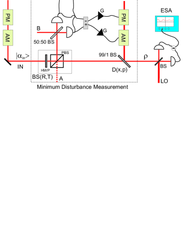
Figure 3: The Experimental Scheme. AM: Amplitude Modulator; PM: Phase Modulator; $|\alpha\rangle$: The incoming coherent state to be measured; HWP: Half Wave Plate; PBS: Polarizing Beam Splitter Cube; BS: Beam Splitter; D(x,p): Displacement operation; B: Auxiliary beam; BS(R,T): Variable beam splitter with reflectivity $R$ and transmissivity $T$ for intensity; A: Vacuum mode; G: electronic gains; $x_{\rm cl},p_{\rm cl}$: classical measurement outcomes; $\rho$: output state; LO: Local Oscillator Beam; ESA: Electronic Spectrum Analyzer.

In this scheme the input mode “in” is mixed with an auxiliary vacuum mode $A$ on an unbalanced beam splitter with amplitude reflectivity $\sqrt{R}$ and transmissivity $\sqrt{T}$ ($R+T=1$). The reflected mode “in” and the transmitted mode $A$ are described by the following quadratures

$$x_{\rm in}^{\prime} = \sqrt{R}x_{\rm in}+\sqrt{T}x_{A}^{(0)},\quad p_{\rm in}^{\prime}=\sqrt{R}p_{\rm in}+\sqrt{T}p_{A}^{(0)},$$

$$x_{A}^{\prime} = \sqrt{T}x_{\rm in}-\sqrt{R}x_{A}^{(0)},\quad p_{A}^{\prime}=\sqrt{T}p_{\rm in}-\sqrt{R}p_{A}^{(0)}.$$

The mode “in” is then superimposed with another vacuum mode $B$ on a balanced beam splitter and the quadratures $x_{1}\equiv x_{\rm in}^{\prime\prime}=(x_{\rm in}^{\prime}+x_{B}^{(0)})/\sqrt{2}$ and $p_{2}\equiv p_{A}^{\prime}=(p_{\rm in}^{\prime}-p_{B}^{(0)})/\sqrt{2}$ are measured at its outputs. After rescaling the measured quadratures $x_{1}$ and $p_{2}$ by the factor $\sqrt{2/R}$ we arrive at the variables $x_{\rm cl}$ and $p_{\rm cl}$ in the form (2), where

$$n_{\rm cl,x}=\frac{\sqrt{T}x_{A}^{(0)}+x_{B}^{(0)}}{\sqrt{R}},\quad n_{\rm cl,p}=\frac{\sqrt{T}p_{A}^{(0)}-p_{B}^{(0)}}{\sqrt{R}}.$$ (63)

The outcomes of the measurement $\bar{x}_{1}$ and $\bar{p}_{2}$ are then used to displace the mode $A$ as $x_{A}^{\prime}\rightarrow x_{\rm out}=x_{A}^{\prime}+\sqrt{2}G\bar{x}_{1}$ and $p_{A}^{\prime}\rightarrow p_{\rm out}=p_{A}^{\prime}+\sqrt{2}G\bar{p}_{2}$, where $G$ is the normalized electronic gain. The output quadratures $x_{\rm out}$ and $p_{\rm out}$ are then of the form (1), where the gain reads as

$$g=\sqrt{T}+G\sqrt{R},$$ (64)

and

$$n_{\rm out,x} = \frac{\left(G\sqrt{T}-\sqrt{R}\right)x_{A}^{(0)}+Gx_{B}^{(0)}}{g},$$

$$\quad n_{\rm out,p} = \frac{\left(G\sqrt{T}-\sqrt{R}\right)p_{A}^{(0)}-Gp_{B}^{(0)}}{g}.$$ (65)

Inserting now Eqs. (63) and (V) into the definitions (7) one finds

$$\nu_{\rm cl}=\frac{1+T}{1-T},\quad\nu_{\rm out}=\frac{\left(G\sqrt{T}-\sqrt{R}\right)^{2}+G^{2}}{g^{2}}.$$ (66)

Expressing $g^{2}\nu_{\rm out}$ using the second of equations (66), substituting in the obtained formula for $G$ employing Eq. (64) and making use of the formula $R+T=1$ and the first of equations (66) we finally confirm that the noises (66) indeed satisfy the optimal trade-off (13).

Equations (66) immediately allow us to derive the output noise $\nu_{\rm out}$ for the case with optimized gain. Making use of the first of equations (66) in the formula $g_{\rm opt}=\nu_{\rm cl}/\sqrt{\nu_{\rm cl}^{2}-1}$ one gets the optimal gain

$$g_{\rm opt}=\frac{1+T}{2\sqrt{T}}.$$ (67)

Substituting further the latter expression for $g_{\rm opt}$ into Eq. (64) one finds the electronic gain $G_{g_{\rm opt}}$ to be $G_{g_{\rm opt}}=\sqrt{1-T}/2\sqrt{T}$. Inserting now Eq. (67) and the obtained expression for $G_{g_{\rm opt}}$ into the second of equations (66) we finally arrive at the output noise in the linear optics scheme with the feed-forward in the form

$$\nu_{\rm out}=\frac{1-T}{1+T}.$$ (68)

Comparison of the formula for $\nu_{\rm out}$ just obtained with the formula for the noise $\nu_{\rm cl}$ given in Eq. (66) reveals that $\nu_{\rm cl}\nu_{\rm out}=1$ holds and therefore the third of inequalities (8) is saturated.

VI Experiment

After the theoretical part where we proved the optimality of the scheme depicted in Fig. 3 we now proceed by describing the actual experiments demonstrating minimal disturbance measurements (MDMs) on coherent states. As mentioned above, a MDM was recently performed on coherent states Andersen_06 in which the output signal had the same mean value as the input. The present work extends this previous work to a more complete experimental study of MDMs of coherent states namely to the cases where the mean value of the input state is not preserved. We systematically investigated two cases. First, we considered the non-unity gain phase-insensitive MDM where the gain was optimized according to the formula (67). In the second case we studied the non-unity gain MDM where the optical gain was fixed.

The experimental setup is depicted in Fig. 3. In both experiments we used a stable continuous wave Nd:YAG laser from Innolight oscillating at 1064 nm wavelength which could deliver up to 500 mW of power in one transversal mode. The signal beam, local oscillator (LO) beam and the auxiliary beam (B) were all obtained from this source enabling high quality mode matching between the beams and hence allowing very efficient quantum measurements. We generated the coherent states by placing concatenated electro-optical phase and amplitude modulators in the beam path. We applied a signal to the modulators at 14.3 MHz which created sidebands with respect to the laser carrier, meaning that some of the photons from the carrier were transferred to these sidebands. Hence we defined our coherent state to reside at the sideband frequency of 14.3 MHz and having a 100 kHz bandwidth. In this operating window the dark noise of the detectors was negligible and the locking loops for the amplitude and phase quadrature measurement at the homodyne detector were optimized to operate stably. In addition, the feed-forward loop was chosen to function most efficiently inside this window. After the preparation, the coherent state impinges on a beam splitter BS(R,T) with variable beam splitting ratio. The variable beam splitter is realized by placing a polarizing beam splitter behind a half wave plate in the beam path. The reflected part of the input state is mixed with an auxiliary beam of equal intensity on a 50:50 beam splitter. By directly measuring the output of the beam splitter and subsequently constructing the sum and difference photocurrents, the amplitude and phase quadratures of the reflected light are simultaneously measured leuchs99 , thus information about the input is acquired. The classical measurement outcome is amplified electronically and fed to another pair of amplitude and phase modulators which are traversed by another auxiliary beam. This beam is then coupled into the remaining part of the signal beam thus accomplihing a lossless displacement operation. The output state $\rho$ is finally analyzed by making use of a homodyne detector. A bright local oscillator beam interferes with the signal beam on a beam splitter, and the conjugate quadratures, amplitude and phase, are stably measured by locking the relative phase between the two beams employing standard electronic feedback techniques. The first and second moments of the amplitude and phase quadratures of the output state as well as the input state are thus measured using an electronic spectrum analyzer. The input state was characterized by switching off the displacement operation, measuring the resulting output state and inferring the input state by carefully characterizing all the losses including the detector and beam splitter losses. In all the measurements the central frequency was 14.3 MHz, the resolution bandwidth was 100 kHz and the video bandwidth was 30 Hz.

In the first experiment the optical gain of our measurement device depended on the transmission of the beam splitter BS(R,T) according to Eq. (67) thereby reducing the noise $\nu_{\rm out}$ to a minimum possible value. This was achieved by tuning the variable beam splitter to various transmission/reflection ratios and correspondingly adjusting the feed-forward electronic gain to obtain the desired optimal optical gain.

In order to quantify our measurement device and to verify that it indeed measures the coherent state optimally with minimal disturbance we needed to determine the added noises $\langle{n^{2}_{\rm out,x}}\rangle$, $\langle{n^{2}_{\rm out,p}}\rangle$, $\langle{n^{2}_{\rm cl,x}}\rangle$ and $\langle{n^{2}_{\rm cl,p}}\rangle$. For this purpose we measured the Signal to Noise Ratio of the input $\mathrm{SNR}_{\rm in}$ and the Signal to Noise Ratio of the output $\mathrm{SNR}_{\rm out}$ for the conjugate amplitude and phase quadratures, respectively (see e.g. cloning ). The variances of added noises in the output quadratures $\langle{n^{2}_{\rm out,x}}\rangle$ and $\langle{n^{2}_{\rm out,p}}\rangle$ then read as

$$\langle{n^{2}_{\rm out,x}}\rangle = \frac{\mathrm{SNR}_{\rm in,x}}{\mathrm{SNR}_{\rm out,x}}-1,\quad\langle{n^{2}_{\rm out,p}}\rangle=\frac{\mathrm{SNR}_{\rm in,p}}{\mathrm{SNR}_{\rm out,p}}-1.$$

The variances $\langle{n^{2}_{\rm cl,x}}\rangle$ and $\langle{n^{2}_{\rm cl,p}}\rangle$ of the noises added into the classical measurement outcomes were calculated from the measured transmittance $T$ of the variable beam splitter. By construction, the device should exhibit identical transmittance for the amplitude and phase quadratures, and this was explicitly confirmed by measurement. We thus have

$$\nu_{\mathrm{cl}}=\langle{n^{2}_{\rm cl,x}}\rangle=\langle{n^{2}_{\rm cl,p}}\rangle=\frac{1+T}{1-T}.$$ (70)

Simultaneously changing the transmittance T and the electronic gain G enabled us to adjust at will the degree of disturbance of the measured quantum state. The experimental results are summarized in Fig. 4. We get excellent agreement between theory and experiment and we conclude that the measurement apparatus operates at the fundamental limits imposed by quantum theory.

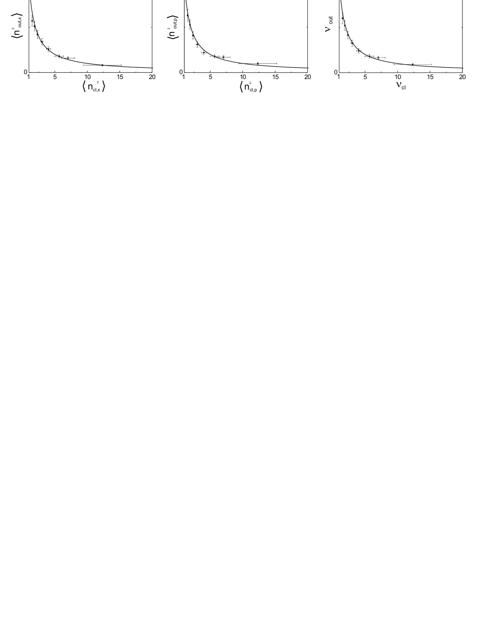
Figure 4: Experimental results for MDM with optimized gain. Variances $\langle n^{2}_{\rm out,x}\rangle$ (left figure) and $\langle n^{2}_{\rm out,p}\rangle$ (middle figure) of the added noises in the amplitude and phase quadratures are plotted against the quantity $\langle n^{2}_{\rm cl,x}\rangle$ and $\langle n^{2}_{\rm cl,p}\rangle$ characterizing the noise added into the outcomes of simultaneous measurement of amplitude and phase quadratures. We also make use of Eq.(7) to plot $\nu_{\rm out}$ against $\nu_{\rm cl}$ (right figure). The solid line represents the theoretical relation $\nu_{\rm out}=1/\nu_{\rm cl}$. The experimental data were obtained by taking into account the detection efficiency of $83\%$ at the homodyne detector. The error bars in the $x$-axis steam from the uncertainty in the measurement of the beam splitter transmission ($2\%$ deviation). The error bars in the $y$-axis are caused by 0.1 dB relative measurement accuracy of the Electronic Spectrum Analyzer and 0.1 dB deviation of the homodyning efficiency.

In our second experiment we demonstrated the MDM for a fixed optical gain. After analyzing our input state as in the previous experiment we connected the feed-forward loop and adjusted the appropriate electronic gain which guaranteed the desired fixed optical gain. This means that for a particular beam splitter transmission the feed-forward electronic gain will increase as the desired optical gain increases. If, in addition, the desired optical gain is less than the beam splitter transmission then a deamplification of the optical signal is required which was achieved by adding a $\pi$ phase shift in the electronic feed-forward loop and by making use of destructive interference which resulted in optical deamplification. This particular operation is actually suboptimal meaning that the measurement outcomes lie outside the optimality window which follows directly from the fact that in this case where $g<\sqrt{T}$, calculation of $\nu_{\rm cl}$ reveals that $\nu_{\rm cl}>(1+g^{2})/|1-g^{2}|$. Using a similar procedure as before we measured the first and second moments for the amplitude and phase quadrature of the output signal. Having measured the input and output states we then calculate all the necessary added noises by means of Eqs. (VI) and (70).

Figure 5: Experimental results for MDM with fixed gains $g^{2}=0.5$ (a), $g^{2}=0.8$ (b) and $g^{2}=1.3$ (c). Variances $\langle n^{2}_{\rm out,x}\rangle$ (left figure) and $\langle n^{2}_{\rm out,p}\rangle$ (middle figure) of the added noises in the amplitude and phase quadratures are plotted against the $\langle n^{2}_{\rm cl,x}\rangle$ and $\langle n^{2}_{\rm cl,p}\rangle$ characterizing the noise added into the outcomes of simultaneous measurement of amplitude and phase quadratures. We also make use of Eq.(7) to plot $\nu_{\rm out}$ against $\nu_{\rm cl}$ (right figure). The optimality windows (gray shaded regions) are determined by Eqs. (14) and (15). The solid line represents the theoretical trade-off (13). The experimental data were obtained by taking into account the detection efficiency of $83\%$ at the homodyne detector. The error bars in the $x$-axis stem from the uncertainty in the measurement of the beam splitter transmission ($2\%$ deviation). The error bars in the $y$-axis are caused by 0.1 dB relative measurement accuracy of the Electronic Spectrum Analyzer and 0.1 dB deviation of the homodyning efficiency.

We performed this kind of measurement for three fixed optical gains of $g^{2}=0.5,0.8,1.3$ and the results are summarized in Fig. 5. Here we have to stress again that optimal MDMs with a fixed optical gain lie only within a specific region of the $(\nu_{\rm cl},\nu_{\rm out})$-plane (gray shaded region in the figures). The boundaries of these regions depend solely on the optical gain and can be easily determined from Eqs. (14) and (15). For the optical gains considered here these optimality windows explicitly read as follows:

$$1\leq\nu_{\rm cl}\leq 3, \quad 1\leq\nu_{\rm out}\leq 3\quad\mbox{for $g^{2}=0.5$},$$

$$1\leq\nu_{\rm cl}\leq 9, \quad\frac{1}{4}\leq\nu_{\rm out}\leq\frac{9}{4}\quad\mbox{for $g^{2}=0.8$},$$

$$1\leq\nu_{\rm cl}\leq\frac{23}{3}, \quad\frac{3}{13}\leq\nu_{\rm out}\leq\frac{23}{13}\quad\mbox{for $g^{2}=1.3$}.$$

The left hand sides of these inequalities are dictated by the commutation relations (II) and cannot be overcome by any operation, i.e. the theoretical trade-off in the figures never lies below or to the left of the optimality window. However, the trade-off (13) lies to the right of the optimality window for sufficiently large noise $\nu_{\rm cl}$. In this case the operation saturating the trade-off is suboptimal and a better performance is obviously obtained by the operation corresponding to the minimum of the trade-off which also corresponds to the bottom right corner of the optimality window. Note that the only exception occurs in the unity gain regime ($g=1$) demonstrated in Andersen_06 where the optimality window is not bounded from the right, i.e.

$$1\leq\nu_{\rm cl}\leq\infty,\quad 0\leq\nu_{\rm out}\leq 2.$$ (71)

Thus, since $\nu_{\rm cl}-\sqrt{\nu_{\rm cl}^{2}-1}\leq 1$ for any $\nu_{\rm cl}\geq 1$ the optimal output noise $\nu_{\rm out}$ for $g=1$ always satisfies the second inequality in (71) and therefore in the unity gain regime the trade-off (13) never leaves the optimality window.

As can be seen in Fig. 5, the obtained experimental trade-offs are in very good agreement with the theory which shows that our measuring apparatus indeed realizes optimal non-unity gain Gaussian partial estimation of coherent states. In particular, the noises added to the phase and amplitude quadratures are practically the same, which confirms that the measurement procedure introduces isotropic phase-independent noise into the estimated state as well as the post-measurement state.

VII Discussion and conclusions

Our experimental minimal disturbance measurement with fixed non-unity gain finds a direct application in the context of optimal Gaussian individual attacks on coherent state quantum key distribution (QKD) with heterodyne detection and direct reconciliation Weedbrook_04 . The optimal trade-off demonstrated by us determines the minimum added noise in the outcomes of simultaneous measurement of complementary quadratures a potential eavesdropper can reach for a Gaussian quantum channel with a fixed gain and a fixed phase-insensitive added noise. In the QKD terminology it means that the minimal disturbance measurement provides an eavesdropper with maximum possible information that can be gained from an individual Gaussian attack in the heterodyne-based coherent state QKD protocol with direct reconciliation. Recently, the similar problem has been studied theoretically directly in the context of QKD Lodewyck_07 and another form of the above mentioned trade-off was found (Eq. (11) of Ref. Lodewyck_07 ). The proofs of optimality presented here, however, follow completely different strategies in comparison with those presented in Lodewyck_07 and more importantly we saturate the optimal trade-off between added noises experimentally.

In this article we have extended the concept of the phase-insensitive MDM for coherent states to the non-unity gain regime. We have given a complete theoretical as well as experimental study of this MDM for two different scenarios. First, we have found the non-unity gain MDM assuming fixed optical gain. In the second scenario we considered MDM with optimized gain. We have shown that both MDMs can be realized by a scheme consisting of only linear optical elements and a feed-forward and we implemented the scheme experimentally. We have experimentally reached theoretical limits in both scenarios. Our results give answer to a fundamental question of how much noise will be in the measurement outcomes from the non-destructive measurement of a coherent state provided that it is represented by a single-mode Gaussian channel with a given optical gain and isotropic added noise. Our analysis could be also extended to phase-sensitive measurements such as the quantum non-demolition measurement of a single quadrature of light.

- (1) K. Banaszek and I. Devetak, Phys. Rev. A 64, 052307 (2001).
- (2) K. Banaszek, Phys. Rev. Lett. 86, 1366 (2001).
- (3) L. Mišta, Jr., J. Fiurášek, and R. Filip, Phys. Rev. A 72, 012311 (2005).
- (4) L. Mišta, Jr. and J. Fiurášek, Phys. Rev. A 74, 022316 (2005).
- (5) M.F. Sacchi, Phys. Rev. Lett. 96 220502 (2006).
- (6) H. Barnum, eprint quant-ph/0205155 (2002).
- (7) C.A. Fuchs and A. Peres, Phys. Rev. A 53, 2038 (1996).
- (8) L. Maccone, Phys. Rev. A 73, 042307 (2006).
- (9) F. Sciarrino, M. Ricci, F. De Martini, R. Filip, and L. Mišta, Jr., Phys. Rev. Lett. 96, 020408 (2006).
- (10) U. L. Andersen, M. Sabuncu, R. Filip, and G. Leuchs, Phys. Rev. Lett. 96, 020409 (2006).
- (11) L. Mišta Jr., Phys. Rev. A, 73, 032335, (2006).
- (12) M.G. Genoni and M.G.A. Paris, Phys. Rev. A 74, 012301 (2006).
- (13) Stefano Olivares and Matteo G. A. Paris, quant-ph/0611272
- (14) N.J. Cerf, G. Leuchs and E.S. Polzik (Eds.), Quantum information with continuous variables of atoms and light, Imperial College Press, London (2007).
- (15) S. L.Braunstein and P. van Loock, Rev. Mod. Phys. 77, 513 (2005).
- (16) J.-H. Poizat, J.-F. Roch, and P. Grangier, Ann. Phys. (Paris) 19, 265 (1994).
- (17) T. C. Ralph, Phys. Rev. A 62, 062306 (2000).
- (18) C. Weedbrook, A. M. Lance, W. P. Bowen, T. Symul, T. C. Ralph, and P. K. Lam, Phys. Rev. Lett. 93, 170504 (2004); A. M. Lance, T. Symul, V. Sharma, C. Weedbrook, T. C. Ralph, and P.K. Lam Phys. Rev. Lett. 95, 180503 (2005).
- (19) S. Lorenz, N. Korolkova and G. Leuchs, Appl. Phys. B 79 (2004). S. Lorenz, J. Rigas, M. Heid, U.L. Andersen, N. Lütkenhaus, and G. Leuchs, Phys. Rev. A 74, 042326(2006).
- (20) L. Vaidman, Phys. Rev. A 49, 1473 (1994).
- (21) S. L. Braunstein and H. J. Kimble, Phys. Rev. Lett. 80, 869 (1998).
- (22) A. Furusawa, J. L. Sørensen, S. L. Braunstein, C. A. Fuchs, H. J. Kimble, and E. S. Polzik, Science 282, 706 (1998); W. P. Bowen, N. Treps, B. C. Buchler, R. Schnabel, T. C. Ralph, H.-A. Bachor, T. Symul, and P. K. Lam, Phys. Rev. A 67, 032302 (2003); T. C. Zhang, K. W. Goh, C. W. Chou, P. Lodahl, and H. J. Kimble, Phys. Rev. A 67, 033802 (2003).
- (23) W. P. Bowen, N. Treps, B. C. Buchler, R. Schnabel, T. C. Ralph, T. Symul, and P. K. Lam, IEEE J. Sel. Top. Quant. 9, 1519 (2003).
- (24) L. Vandenberghe and S. Boyd, SIAM Rev. 38, 49 (1996).
- (25) A. C. Doherty, P. A. Parillo, and F. M. Spedalieri, Phys. Rev. Lett. 88, 187904 (2002).
- (26) P. Hyllus and J. Eisert, New J. Phys. 8, 51 (2006).
- (27) K. Audenaert and B. De Moor, Phys. Rev. A 65, 030302(R) (2002).
- (28) F. Verstraete and H. Verschelde, Phys. Rev. A 66, 022307 (2002); Phys. Rev. Lett. 90, 097901 (2003).
- (29) M. Ježek, J. Řeháček, and J. Fiurášek, Phys. Rev. A 65, 060301(R) (2002).
- (30) Y. C. Eldar, A. Megretski, and G. C. Verghese, IEEE Trans. Inf. Theory 49, 1007 (2003).
- (31) J. Fiurasek and N.J. Cerf, Phys. Rev. A 75, 052335 (2007).
- (32) G. Leuchs,T.C. Ralph,C. Silberhorn, N. Korolkova, Journal of Modern Optics. 46, 1927 (1999).
- (33) U.L. Andersen, V. Josse and G. Leuchs, Phys. Rev. Lett. 94 240503 (2005).
- (34) J. Lodewyck and P. Grangier, e-print quant-ph/07041371 (2007).