Renormalized Newtonian Cosmic Evolution with Primordial Non-Gaussianity

Abstract

We study Newtonian cosmological perturbation theory from a field theoretical point of view. We derive a path integral representation for the cosmological evolution of stochastic fluctuations. Our main result is the closed form of the generating functional valid for any initial statistics. Moreover, we extend the renormalization group method proposed by Mataresse and Pietroni to the case of primordial non-Gaussian density and velocity fluctuations. As an application, we calculate the nonlinear propagator and examine how the non-Gaussianity affects the memory of cosmic fields to their initial conditions. It turns out that the non-Gaussianity affect the nonlinear propagator. In the case of positive skewness, the onset of the nonlinearity is advanced with a given comoving wavenumber. On the other hand, the negative skewness gives the opposite result.

I Introduction

The large scale structure in the universe has evolved from primordial fluctuations according to the gravitational instability. In the standard scenario of the structure formation, the primordial fluctuations are created quantum mechanically during the inflationary stage in the early universe. After exiting the horizon, the fluctuations are evolved linearly; which is well described by relativistic linear perturbation theory. Eventually the fluctuations re-enter into the horizon. After that, it is sufficient to treat the evolution of fluctuations by means of Newtonian gravity. Due to the Jeans instability, at some point, the density fluctuations become nonlinear. In this stage, usually we resort to the N-body simulations. However, since the numerical simulations are time consuming, the analytical calculation of the nonlinear evolution is still desired. The standard perturbative expansion method is developed for this purpose. In the quasi-nonlinear regime, the perturbative approach was successful Suto:1990wf ; Makino:1991rp ; Jain:1993jh ; Scoccimarro:1995if ; Sahni:1995rm ; Matsubara:2000mw ; Bernardeau:2001qr . To obtain more accurate results, however, the non-perturbative analytic method would be necessary.

Recently, Crocce and Scoccimarro have developed a new formalism to study the large scale structure Crocce:2005xy . They described the perturbative solution by Feynman diagrams and identified three fundamental objects: the initial conditions, the vertex, and the propagator. They have found that the renormalization of the propagator is the most important one. Based on this finding, they have observed that, due to the rapid fall off of the nonlinear propagator, the memory of the cosmic fields to their initial conditions will be lost soon in the nonlinear regime.

Following their work, Matarrese and Pietroni reformulated the cosmological perturbation theory from the path integral point of view and developed the renormalization group (RG) techniques in cosmology Matarrese:2007aj ; Matarrese:2007wc ( see McDonald:2006hf for a slightly different approach). Matarrese and Pietroni have applied their formalism to the baryon acoustic oscillations (BAO) which takes place around the scale $k\sim 0.1{\rm Mpc}^{-1}$ Eisenstein:2005su . On these scales, the nonlinear effects are relevant Huff:2006gs ; Jeong:2006xd . They have found that the renormalization group method is useful to predict the BAO feature. Crocce and Scoccimarro have used their graphical approach to discuss BAO and found the renormalized perturbation approach gives a good agreements with results of numerical simulations Crocce:2007dt . This result is further confirmed by Nishimichi et al. Nishimichi:2007xt .

These authors have discussed only the Gaussian initial conditions. Recently, however, it has been realized that the primordial non-Gaussianity can be produced in the inflationary scenario. If so, it is important to give a renormalization group formalism for the non-Gaussian initial conditions. Conventionary, the non-Gaussian curvature perturbation $\Phi$ is characterized by the following form

$$\Phi({\bf x})=\Phi_{g}({\bf x})+f_{NL}(\Phi_{g}^{2}({\bf x})-\langle\Phi_{g}^{2}\rangle),$$ (1)

where $\Phi_{g}$ is the Gaussian field and $f_{NL}$ is the parameter to represent a deviation from the Gaussianity. There are several possible observational tests to constrain the non-Gaussianity Koyama:1999fc ; Willick:1999ty ; Robinson:1999wh ; Matarrese:2000iz ; Scoccimarro:2000qg ; Seto:2001mg ; Scoccimarro:2003wn ; Hikage:2006fe ; Sefusatti:2006eu . The most stringent limit comes from WMAP and the result is $-58<f_{NL}<134$ Komatsu:2003fd . Planck and other tests will give a more stringent limit or detect the non-Gaussianity Bartolo:2004if .

The purpose of this paper is therefore to extend the analysis by Matarrese and Pietroni to the non-Gaussian initial conditions. Starting from the generating functional of the multi-point functions, we derive the path integral representation of the cosmic evolution of the cosmic fields. In contrast to the previous work, the non-Gaussianity is incorporated into the field theoretical scheme. In particular, we obtain the formula for the generating functional which allows us to use the Feynman diagram method to calculate various statistical quantities characterizing the large scale structure in the universe. We also derive the RG equation for the effective action. As an application, we calculate the nonlinear propagator and examine if the memory of the cosmic fields to their initial conditions has the tendency to be kept by the non-Gaussianity or not.

The organization of this paper is as follows. In section II, we review the basic equations of motion describing the evolution of the cosmic fields. In section III, we develop the general field theoretical framework so that the non-Gaussianity can be incorporated into the scheme. We have successfully calculated the generating functional which gives Feynman rules. We also develop the renormalization group method in this context. In section IV, we apply our formalism to calculate the nonlinear propagator for the non-Gaussian initial conditions and examine the effect of non-Gaussianity on the nonlinear scales. The final section is devoted to the conclusion.

II Basic equations for cosmic fields

In this section, we review the standard Newtonian cosmological perturbation theory. Here, we consider the Einstein-de Sitter universe for simplicity. Of course, it is possible to extend our analysis to other cosmological models.

First of all, let us consider the homogeneous cosmological background spacetime. Taking the conformal time and assuming the flat space, we can write down the metric

$$ds^{2}=a^{2}(\tau)\left[-d\tau^{2}+\delta_{ij}dx^{i}dx^{j}\right]\ .$$ (2)

The cosmological scale factor $a$ is determined by solving FRW equations

$${\cal H}^{2}=\frac{8\pi G}{3}a^{2}\rho_{0}\ ,\quad{\cal H}^{\prime}=-\frac{4\pi G}{3}a^{2}\rho_{0}\ ,$$ (3)

where $\rho_{0}$ is the averaged density field and we have defined ${\cal H}=da/d\tau/a=a^{\prime}/a$.

Now, let us consider the inhomogeneous distribution of the matter. The evolution of the total matter density is determined by the gravity including the effect of cosmic expansion. The actual density $\rho({\bf x},\tau)$ is deviated from the averaged density $\rho_{0}(\tau)$ Let us define the density fluctuation as

$$\delta({\bf x},\tau)=\frac{\rho({\bf x},\tau)-\rho_{0}(\tau)}{\rho_{0}(\tau)}=\int d^{3}k\delta({\bf k},\tau)e^{-i{\bf k}\cdot{\bf x}}\ .$$ (4)

It obeys the equation of continuity and the peculiar velocity ${\bf v}$ is determined by the Euler equation in the presence of gravitational potential $\phi$. The gravitational potential itself is governed by the Poisson equation. Thus, equations of motion for the cosmic fields, $\delta$, ${\bf v}$, and $\phi$, are given by

$$\frac{\partial\delta}{\partial\tau}+\nabla\cdot\left[\left(1+\delta\right){\bf v}\right]=0,$$ (5)

$$\frac{\partial{\bf v}}{\partial\tau}+{\cal H}{\bf v}+\left({\bf v}\cdot\nabla\right){\bf v}=-\nabla\phi,$$ (6)

$$\nabla^{2}\phi=\frac{3}{2}{\cal H}^{2}\delta\ .$$ (7)

On large scales, the assumption that the peculiar velocity is irrotational would be valid. Then, defining $\theta=\nabla\cdot{\bf v}$, we obtain the relation ${\bf v}({\bf k},\tau)=i{\bf k}\theta({\bf k},\tau)/k^{2}$. After eliminating the gravitational potential, we obtain equations of motion in the Fourier space

$$\frac{\partial\delta({\bf k},\tau)}{\partial\tau}+\theta({\bf k},\tau)+\int d^{3}{\bf q}d^{3}{\bf p}\delta_{D}({\bf k}-{\bf q}-{\bf p})\alpha({\bf q},{\bf p})\theta({\bf q},\tau)\delta({\bf p},\tau)=0,$$ (8)

$$\frac{\partial\theta({\bf k},\tau)}{\partial\tau}+{\cal H}\theta({\bf k},\tau)+\frac{3}{2}{\cal H}^{2}\delta({\bf k},\tau)$$

$$\qquad+\int d^{3}{\bf q}d^{3}{\bf p}\delta_{D}({\bf k}-{\bf q}-{\bf p})\beta({\bf q},{\bf p})\theta({\bf q},\tau)\theta({\bf p},\tau)=0,$$ (9)

where we have defined the Dirac delta function $\delta_{D}$ and

$$\alpha({\bf q},{\bf p})=\frac{({\bf p}+{\bf q})\cdot{\bf q}}{q^{2}}\ ,\quad\beta({\bf q},{\bf p})=\frac{({\bf p}+{\bf q})^{2}{\bf p}\cdot{\bf q}}{2p^{2}q^{2}}$$ (10)

characterize the nonlinear gravitational coupling.

It is now easy to solve the above equations perturbatively. Given the expansion

$$\delta({\bf k},\tau)=\sum_{n=1}^{\infty}\delta^{(n)}({\bf k},\tau)\ ,\quad\theta({\bf k},\tau)=\sum_{n=1}^{\infty}\theta^{(n)}({\bf k},\tau)\ ,$$ (11)

the iterative solutions can be explicitly written down as functional of the initial fields Bernardeau:2001qr . Once the probability functional for the initial fields are given, one can calculate expectation values of product of these fields. In fact, this standard formalism has been utilized to calculate the quasi-nonlinear evolution of the power spectrum, bispectrum, and other statistics such as genus statistics Sahni:1995rm ; Matsubara:2000mw ; Bernardeau:2001qr . In the nonlinear regime, however, further analytical tools are required to give more accurate results. This is crucial for the prediction of BAO feature, for example. In the next section, we introduce a useful approach to this end.

III Path Integral Formalism and Renormalization Group

Now, we proceed to formulate the cosmological perturbation theory in the field theoretical manner. Doing so, we can utilize the idea invented in the field theory. In particular, the renormalization group method turns out to be useful.

As is suggested by Crocce and Scoccimarro Crocce:2005xy , the equations of motion can be rewritten in a convenient form by defining a two-component vector

$$\varphi_{a}({\bf k},\tau)\equiv\left(\begin{array}[]{c}\varphi_{1}({\bf k},\tau)\\ \varphi_{2}({\bf k},\tau)\end{array}\right)\equiv e^{-\eta}\left(\begin{array}[]{c}\delta({\bf k},\tau)\\ -\theta({\bf k},\tau)/{\cal H}\end{array}\right),$$ (16)

where the index $a=1,2$ and $\eta=\log a(\tau)/a_{\rm in}$ denotes the e-folding number. The initial scale factor $a_{\rm in}$ can be taken arbitrarily. We also define vertex $\gamma_{abc}$ with

$$\gamma_{121}({\bf k},{\bf p},{\bf q})=\frac{1}{2}\delta_{D}({\bf k}+{\bf p}+{\bf q})\alpha({\bf p},{\bf q})=\gamma_{112}({\bf k},{\bf q},{\bf p})\ ,\quad\gamma_{222}({\bf k},{\bf p},{\bf q})=\delta_{D}({\bf k}+{\bf p}+{\bf q})\beta({\bf p},{\bf q})$$ (17)

and other components are zero. Using the above definitions, we obtain the equation

$$\left(\delta_{ab}\partial_{\eta}+\Omega_{ab}\right)\varphi_{b}({\bf k},\eta)=e^{\eta}\gamma_{abc}({\bf k},-{\bf p},-{\bf q})\varphi_{b}({\bf p},\eta)\varphi_{c}({\bf q},\eta),$$ (18)

where $\Omega_{ab}$ are components of the matrix

$$\Omega=\left(\begin{array}[]{cc}1&-1\\ -3/2&3/2\end{array}\right).$$ (21)

Here, we have used the Einstein’s sum rule

$$\varphi_{a}(-{\bf k},0)\varphi_{b}({\bf k},0)\equiv\int d^{3}k\varphi_{a}(-{\bf k},0)\varphi_{b}({\bf k},0)\ .$$ (22)

From now on, we should understand this convention is used when the same wavenumber vector appear twice in the same term.

First, we consider the linear theory. The growing and the decaying modes can be written as $u_{a}$ and $v_{a}\exp(-5\eta/2)$, respectively. Here, we have defined two basis vectors

$$u_{a}=\left(\begin{array}[]{c}1\\ 1\\ \end{array}\right)\qquad\mbox{and}\qquad v_{a}=\left(\begin{array}[]{c}1\\ -3/2\\ \end{array}\right).$$ (27)

Let us define the linear propagator as

$$\left(\delta_{ab}\partial_{\eta}+\Omega_{ab}\right)g_{bc}(\eta_{a}-\eta_{b})=\delta_{ac}\delta_{D}(\eta_{a}-\eta_{b})\ .$$ (28)

Given the growing and decaying mode functions, we can write down the causal propagator $g_{ab}$ as

$$g_{ab}(\eta_{a},\eta_{b})=\left\{u_{a}\hat{u}_{b}+v_{a}\hat{v}_{b}\exp{(-5/2(\eta_{a}-\eta_{b}))}\right\}\theta(\eta_{a}-\eta_{b}),$$ (29)

where $\hat{u}_{a}$ and $\hat{v}_{a}$ are dual vectors of $u_{a}$ and $v_{a}$,

$$\hat{u}_{a}=\frac{1}{5}(3,2)\qquad\mbox{and}\qquad\hat{v}_{a}=\frac{2}{5}(1,-1).$$ (30)

Note that we have the matrix components

$$u_{a}\hat{u}_{b}=\frac{1}{5}\left(\begin{array}[]{cc}3&2\\ 3&2\end{array}\right)\ ,\quad v_{a}\hat{v}_{b}=\frac{1}{5}\left(\begin{array}[]{cc}2&-2\\ -3&3\end{array}\right).$$ (35)

Using this linear propagator, we can formally solve the equation (18) as

$$\varphi_{a}({\bf k},\eta_{a})=g_{ab}(\eta_{a},0)\varphi_{b}({\bf k},0)+\int d\eta_{b}g_{ab}(\eta_{a},\eta_{b})e^{\eta}\gamma_{bcd}({\bf k},-{\bf p},-{\bf q})\varphi_{c}({\bf p},\eta_{b})\varphi_{d}({\bf q},\eta_{b})\ .$$ (36)

Iteration gives the perturbative solutions. There are three building blocks, the initial field $\varphi({\bf k},0)$, the linear propagator $g_{ab}$, and the vertex $\gamma_{abc}$. The initial field is usually assumed to have Gaussian statistics characterized by the linear power spectrum

$$<\varphi({\bf k},0)\varphi({\bf k}^{\prime},0)>=(2\pi)^{3}\delta_{D}({\bf k}+{\bf k}^{\prime})P_{ab}^{L}\ .$$ (37)

The nonlinear power spectrum can be calculated using the graphical method as was first demonstrated by Crocce and Scoccimarro Crocce:2005xy . In particular, the renormalization method is utilized to perform the partial sum of diagrams. It turned out the approximation motivated by the renormalization method was quite successful Afshordi:2006ch . In the next subsection, we consider more general statistics for the initial field $\varphi_{a}({\bf k},0)$.

III.1 Path Integral Representation

What we are interested in are the statistical quantities characterizing the large scale structure in the universe. The statistics of primordial cosmic fields $\varphi_{a}({\bf k},0)$ are determined by the initial probability functional $P[\varphi_{a}({\bf k},0)]$. To calculate desired quantities, we need to solve the nonlinear evolution equations and obtain the solution as a function of the initial fields. Namely, we have the statistics and the dynamics to be considered. More precisely, we want to calculate

$$\left<\exp i\int d\eta J_{a}(-{\bf k},\eta)\varphi_{a}({\bf k},\eta;\varphi({\bf k},0))\right>$$

$$\qquad=\int d\varphi_{a}({\bf k},0)P[\varphi_{a}({\bf k},0)]\exp i\int d\eta J_{a}(-{\bf k},\eta)\varphi_{a}({\bf k},\eta;\varphi_{a}({\bf k},0)),$$ (38)

where $P[\varphi_{a}({\bf k},0)]$ is the general probability functional for the initial field $\varphi_{a}({\bf k},0)$ and $\varphi_{a}({\bf k},\eta;\varphi_{a}({\bf k},0))$ is the solution of Eq.(18) with the initial condition $\varphi_{a}({\bf k},0)$. This is a generating functional for multi-point correlation functions. Here, we shall combine the statistics and the dynamics in a unified framework. This can be achieved by the field theoretical path integral method. It is the path integral representation of the problem which can be used to perform the non-perturbative approximation.

To derive the path integral representation for the cosmic fields starting from the expression (38), we introduce an auxiliary field $\varphi_{a}({\bf k},\eta)$ as

$$\int d\varphi_{a}({\bf k},0)\int D\varphi_{a}({\bf k},\eta)P[\varphi_{a}({\bf k},0)]\delta_{D}(\varphi_{a}({\bf k},\eta)-\varphi_{a}({\bf k},\eta;\varphi({\bf k},0)))\exp i\int d\eta J_{a}(-{\bf k},\eta)\varphi_{a}({\bf k},\eta)\ ,$$ (39)

where we used the Dirac delta function $\delta_{D}$. To separate the dynamics from the statistics, we use the operator ${\bf L}$ defined by

$${\bf L}\varphi_{a}=\left(\delta_{ab}\partial_{\eta}+\Omega_{ab}\right)\varphi_{b}({\bf k},\eta)-e^{\eta}\gamma_{abc}({\bf k},-{\bf p},-{\bf q})\varphi_{b}({\bf p},\eta)\varphi_{c}({\bf q},\eta)\ .$$ (40)

Then, we get

$$\int d\varphi_{a}({\bf k},0)\int D\varphi_{a}({\bf k},\eta)P[\varphi_{a}({\bf k},0)]\delta_{D}({\bf L}\varphi_{a}({\bf k},\eta)-\varphi_{a}({\bf k},0)\delta_{D}(\eta))\exp i\int d\eta J_{a}(-{\bf k},\eta)\varphi_{a}({\bf k},\eta),$$ (41)

where we have used the fact $\det{\bf L}=1$ valid for the causal boundary conditions Valageas:2006bi . Here, it is convenient to introduce another auxiliary field $\chi_{a}$ to exponentiate the Dirac delta function. This procedure is crucial to integrate out the initial field $\varphi_{a}({\bf k},0)$. The result becomes

$$\int d\varphi_{a}({\bf k},0)\int D\varphi_{a}({\bf k},\eta)D\chi_{a}({\bf k},\eta)P[\varphi_{a}({\bf k},0)]$$ (42)

$$\quad\times\exp\left[i\int d\eta\chi_{a}(-{\bf k},\eta)L\varphi_{a}({\bf k},\eta)-i\chi_{a}(-{\bf k},0)\varphi_{a}({\bf k},0)+i\int d\eta J_{a}(-{\bf k},\eta)\varphi_{a}({\bf k},\eta)\right]$$

$$= \int D\varphi_{a}({\bf k},\eta)D\chi_{a}({\bf k},\eta)e^{C\left[\chi_{a}({\bf k},0)\right]}\exp\left[i\int d\eta\chi_{a}(-{\bf k},\eta){\bf L}\varphi_{a}({\bf k},\eta)+i\int d\eta J_{a}(-{\bf k},\eta)\varphi_{a}({\bf k},\eta)\right],$$

where we have defined the cumulant functional $C[\chi_{a}]$ by

$$e^{C\left[\chi_{a}({\bf k},0)\right]}=\int d\varphi_{a}({\bf k},0)P[\varphi_{a}({\bf k},0)]e^{-i\chi_{a}(-{\bf k},0)\varphi_{a}({\bf k},0)}.$$ (43)

The field $\chi_{a}({\bf k},0)$ is defined as the boundary value of the field $\chi_{a}({\bf k},\eta)$. The cumulant functional completely characterize the initial statistics. It is possible to expand the cumulant as

$$C[\chi_{a}({\bf k},0)]=(2\pi)^{3}\left(-\frac{1}{2}\chi_{a}(-{\bf k},0)P_{ab}\chi_{b}({\bf k},0)+\frac{i}{6}B_{abc}\left({\bf k}_{1},{\bf k}_{2},{\bf k}_{3}\right)\chi_{a}(-{\bf k}_{1},0)\chi_{b}(-{\bf k}_{2},0)\chi_{c}(-{\bf k}_{3},0)+\cdots\right)\ .$$ (44)

The first term is the power spectrum for the initial field. In the Gaussian case, only this term exists. In general, subsequent terms follow. The second term is called the bispectrum

In the above action, the auxiliary field $\chi_{a}$ is introduced as a field. Hence, it is natural to add the source for this field. Thus, we have the final path integral expression for the cosmological fluctuations with the general statistics:

$$Z[J_{a},K_{b}] = \int D\varphi_{a}({\bf k},\eta)D\chi_{a}({\bf k},\eta)e^{C[\chi_{a}({\bf k},0)]}\exp\left[i\int d\eta\chi_{a}(-{\bf k},\eta){\bf L}\varphi_{a}({\bf k},\eta)\right.$$ (45)

$$\left.\qquad+i\int d\eta J_{a}(-{\bf k},\eta)\varphi_{a}({\bf k},\eta)+i\int d\eta K_{a}(-{\bf k},\eta)\chi_{a}({\bf k},\eta)\right].$$

From the field theoretical point of view, $C[\chi_{a}({\bf k},0)]$ can be regarded as the boundary action on the initial hypersurface $\eta=0$. In this sense, the field $\chi_{a}({\bf k},0)$ is associated with the initial conditions.

III.2 Generating functional

Thanks to the auxiliary field $\chi_{a}$, we can perform the path integral completly. First of all, let us extract the nonlinear interaction part

$$Z[J_{a},K_{b}] = \exp iS_{int}[-i\frac{\delta}{\delta J_{a}},-i\frac{\delta}{\delta K_{b}}]\int D\varphi_{a}({\bf k},\eta)D\chi_{a}({\bf k},\eta)e^{C[\chi_{a}({\bf k},0)]}$$ (46)

$$\times\exp\left[i\int d\eta\chi_{a}(-{\bf k},\eta){\bf L}_{lin}\varphi_{a}({\bf k},\eta)+i\int d\eta J_{a}(-{\bf k},\eta)\varphi_{a}({\bf k},\eta)+i\int d\eta K_{a}(-{\bf k},\eta)\chi_{a}({\bf k},\eta)\right]\ ,$$

where ${\bf L}_{lin}$ is the linear part of ${\bf L}$ and $S_{int}$ denotes the interaction part of the action. As the field $\varphi_{a}$ is linear in the action, it is easy to integarte out it as

$$\exp iS_{int}[-i\frac{\delta}{\delta J_{a}},-i\frac{\delta}{\delta K_{b}}]\int D\chi_{a}({\bf k},\eta)e^{C[\chi_{a}({\bf k},0)]}\delta_{D}(\chi_{a}{\bf L}_{lin}+J_{a})\exp\left[i\int d\eta K_{a}({\bf k},\eta)\chi_{a}({\bf k},\eta)\right]\ ,$$ (47)

where $\chi_{a}{\bf L}_{lin}\equiv\chi_{b}(\eta_{b})(-\overleftarrow{\partial}_{\eta_{b}}\delta_{ba}+\Omega_{ba})$. The constraint imposed by the Dirac delta function can be solved by using the equation

$$g_{ab}(\eta_{a},\eta_{b})(-\overleftarrow{\partial}_{\eta_{b}}\delta_{bc}+\Omega_{bc})=\delta_{ac}\delta(\eta_{a}-\eta_{b})$$ (48)

as

$$\chi_{a}({\bf k},\eta_{b})=-\int d\eta J_{a}({\bf k},\eta_{a})g_{ab}(\eta_{a},\eta_{b})\ .$$ (49)

Now, it is straightforward to integrate out the field $\chi_{a}$. The final result is given by

$$Z[J_{a},K_{b}] = \exp iS_{int}[-i\frac{\delta}{\delta J_{a}},-i\frac{\delta}{\delta K_{b}}]\exp\left[C[-\int d\eta J_{a}({\bf k},\eta)g_{ab}(\eta,0)]\right.$$ (50)

$$\qquad\qquad\qquad\qquad\qquad\qquad\qquad\left.-i\int d\eta J_{a}(-{\bf k},\eta_{a})g_{ab}(\eta_{a},\eta_{b})K_{b}({\bf k},\eta_{b})\right].$$

This leads to Feynman rules for calculating various quantities. Thus, we have shown that the graphical method is applicable to the evolution problem of cosmological fluctuations with the general non-Gaussian statistics.

It is useful to see a more concrete expression for our path integral representation. In the case of the Gaussian statistics, the cumulant is determined solely by the power spectrum. Therefore, we have a simple expression

$$Z[J_{a},K_{b}]=\exp\left[-i\int d\eta e^{\eta}\gamma_{abc}({\bf k},{\bf p},{\bf q})\left(-i\frac{\delta}{\delta K_{a}({\bf k})}\right)\left(-i\frac{\delta}{\delta J_{b}({\bf p})}\right)\left(-i\frac{\delta}{\delta J_{c}({\bf q})}\right)\right]Z_{0}[J_{a},K_{b}],$$ (51)

where

$$Z_{0}[J_{a},K_{b}] = \exp\left[-\frac{(2\pi)^{3}}{2}\int d\eta_{a}d\eta_{b}J_{a}(-{\bf k},\eta_{a})P_{ab}(\eta_{a},\eta_{b})J_{b}({\bf k},\eta_{b})\right.$$ (52)

$$\left.\qquad-i\int d\eta_{a}d\eta_{b}J_{a}(-{\bf k},\eta_{a})g_{ab}(\eta_{a},\eta_{b})K_{b}({\bf k},\eta_{b})\right].$$

This result coincides with the expression obtained by Matarrese and Pietroni. In the case of the non-Gaussian statistics, we have infinite series of the irredecible correlation functions. In this non-Gaussian cases, the extra contributions read

$$Z_{0}[J_{a},K_{b}] = \exp\left[(2\pi)^{3}\left(-\frac{1}{2}\int d\eta_{a}d\eta_{b}J_{a}(-{\bf k},\eta_{a})P_{ab}^{L}(\eta_{a},\eta_{b})J_{b}({\bf k},\eta_{b})\right.\right.$$ (53)

$$\qquad\left.\left.-\frac{i}{6}\int d\eta_{a}d\eta_{b}d\eta_{c}J_{a}(-{\bf k},\eta_{a})J_{b}(-{\bf k},\eta_{b})J_{c}(-{\bf k},\eta_{c})B_{abc}^{L}\left({\bf k}_{1},{\bf k}_{2},{\bf k}_{3}\right)+\cdots\right.\right)$$

$$\qquad\left.-i\int d\eta_{a}d\eta_{b}J_{a}(-{\bf k},\eta_{a})g_{ab}(\eta_{a},\eta_{b})K_{b}({\bf k},\eta_{b})\right],$$

where we have defined the propagated initial correlation functions

$$P^{L}_{ab}(\eta_{a},\eta_{b})\equiv g_{ac}(\eta_{a},0)g_{bd}(\eta_{b},0)P_{cd},$$ (54)

$$B^{L}_{abc}\left({\bf k}_{1},{\bf k}_{2},{\bf k}_{3},\eta_{a},\eta_{b},\eta_{c}\right)\equiv g_{ad}(\eta_{a},0)g_{be}(\eta_{b},0)g_{cf}(\eta_{c},0)B_{def}\left({\bf k}_{1},{\bf k}_{2},{\bf k}_{3}\right)\ .$$ (55)

The formula (51) gives Feynman rules. In this paper, we will be concentrated on the effect of the initial bispectrum $B_{abc}$.

In the quantum field theory, the generator of the connected Green functions can be written as

$$W[J_{a},K_{b}]=-i\log Z[J_{a},K_{b}]\ .$$ (56)

The expectation values $\phi_{a}$ and $\chi_{a}$ can be defined as

$$\varphi_{a}=\frac{\delta W}{\delta J_{a}},\qquad\chi_{a}=\frac{\delta W}{\delta K_{a}}.$$ (57)

Motivated from the linear expression

$$(2\pi)^{3}P_{ab}^{L}=-i\frac{\delta^{2}W_{0}}{\delta J_{a}\delta J_{b}}\ ,g_{ab}=-\frac{\delta^{2}W_{0}}{\delta J_{a}\delta K_{b}}\ ,(2\pi)^{3}B_{abc}^{L}=\frac{\delta^{3}W_{0}}{\delta J_{a}\delta J_{b}\delta J_{c}}\ ,$$ (58)

we define

$$(2\pi)^{3}P_{ab}=-i\frac{\delta^{2}W}{\delta J_{a}\delta J_{b}}\ ,G_{ab}=-\frac{\delta^{2}W}{\delta J_{a}\delta K_{b}}\ ,(2\pi)^{3}B_{abc}=\frac{\delta^{3}W}{\delta J_{a}\delta J_{b}\delta J_{c}}\ .$$ (59)

Carrying out the Legendre transformation of $W$, we can define the effective action

$$\Gamma[\varphi_{a},\chi_{a}]=W[J_{a}[\varphi_{a},\chi_{a}],K_{a}[\varphi_{a},\chi_{a}]]-\int d\eta d^{3}{\bf k}(J_{a}[\varphi_{a},\chi_{a}]\varphi_{a}+K_{b}[\varphi_{a},\chi_{a}]\chi_{b}).$$ (60)

where

$$J_{a}[\varphi_{a},\chi_{a}]=-\frac{\delta\Gamma}{\delta\phi_{a}}\ ,\quad K_{a}[\varphi_{a},\chi_{a}]=-\frac{\delta\Gamma}{\delta\chi_{a}}\ .$$ (61)

III.3 Renormalization Group

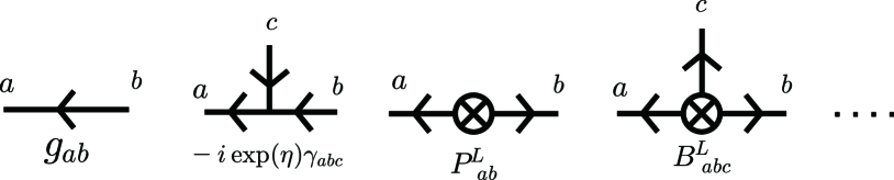
Figure 1: Feymann diagrams; an arrow represents the direction of the time.

The idea of the renormalization group introduced by Matarrese and Pietroni is as follows. First, we introduce a filter function with the UV cutoff $\lambda$ in the $P^{0}_{ab}$ and $B^{0}_{abc}$. This defines a fictious theory where the linear perturbation theory works well. We denote various quantities in the cutoff theory with the suffix $\lambda$, for example like as $P_{ab,\lambda}$. When this cutoff scale $\lambda$ goes to infinity, the original theory is recovered. As $\lambda$ becomes large, nonlinear effects are incorporated gradually. This process can be expressed by the renormalization group equation.

The RG equation for the effective action can be deduced as follows. Taking the derivative of the generating functional $Z_{\lambda}$ with respect to $\lambda$, we obtain

$$\partial_{\lambda}Z_{\lambda} = \frac{(2\pi)^{3}}{2}\int d\eta_{a}d\eta_{b}\partial_{\lambda}P_{ab,\lambda}(p)\delta(\eta_{a})\delta(\eta_{b})\frac{\delta^{2}Z_{\lambda}}{\delta K_{a}(-{\bf p},\eta)\delta K_{b}({\bf p},\eta)}$$ (62)

$$\quad+\frac{(2\pi)^{3}}{6}\int d\eta_{a}d\eta_{b}\eta_{c}\partial_{\lambda}B_{abc,\lambda}({\bf p}_{1},{\bf p}_{2},{\bf p}_{3})\delta(\eta_{a})\delta(\eta_{b})\delta(\eta_{c})\frac{\delta^{3}Z_{\lambda}}{\delta K_{a}({\bf p}_{1},\eta)\delta K_{b}({\bf p}_{2},\eta)\delta K_{c}({\bf p}_{3},\eta)}$$

$$\qquad\qquad\qquad\qquad\qquad\qquad\qquad\qquad\qquad\qquad+\ \cdots,$$

where we have replaced the auxiliary fields $\chi_{a}$ by the functional derivative with repect to $K_{a}$. The above equation can be translated to the equation for the generating functional of the connected Green functions. Using the relation (56), we obtain

$$\partial_{\lambda}W_{\lambda} = \frac{(2\pi)^{3}}{2}\int d\eta_{a}d\eta_{b}\partial_{\lambda}P_{ab,\lambda}\delta(\eta_{a})\delta(\eta_{b})\left(\frac{\delta^{2}W_{\lambda}}{\delta K_{a}(-{\bf p},\eta)\delta K_{b}({\bf p},\eta)}+i\frac{\delta W}{\delta K_{a}(-{\bf p},\eta)}\frac{\delta W}{\delta K_{b}({\bf p},\eta)}\right)$$ (63)

$$\quad+\frac{(2\pi)^{3}}{6}\int d\eta_{a}d\eta_{b}d\eta_{c}\partial_{\lambda}B_{abc,\lambda}({\bf p}_{1},{\bf p}_{2},{\bf p}_{3})\delta(\eta_{a})\delta(\eta_{b})\delta(\eta_{c})$$

$$\quad\times\left(\frac{\delta^{3}W}{\delta K_{a}({\bf p}_{1},\eta)\delta K_{b}({\bf p}_{2},\eta)\delta K_{c}({\bf p}_{3},\eta)}+i\left(\frac{\delta W}{\delta K_{a}({\bf p}_{1},\eta)}\frac{\delta^{2}W}{\delta K_{b}({\bf p}_{2},\eta)\delta K_{c}({\bf p}_{3},\eta)}+(\mbox{cyc}.[a,b,c])\right)\right.$$

$$\qquad\left.-\frac{\delta W}{\delta K_{a}({\bf p}_{1},\eta)}\frac{\delta W}{\delta K_{b}({\bf p}_{2},\eta)}\frac{\delta W}{\delta K_{c}({\bf p}_{3},\eta)}\right)+\ \cdots.$$

Now, we can write down the RG equation for the effective action. Using the definition (60), we get

$$\partial_{\lambda}\Gamma_{\lambda}[\varphi_{a},\chi_{b}]$$

$$\qquad=\partial_{\lambda}W_{\lambda}[J_{\lambda,a}[\varphi_{a},\chi_{b}],K_{\lambda,a}[\varphi_{a},\chi_{b}]]-(\partial_{\lambda}J_{\lambda,a}[\varphi_{a},\chi_{a}]\varphi_{a}+\partial_{\lambda}K_{\lambda,b}[\varphi_{a},\chi_{a}]\chi_{b})$$

$$\qquad=\biggl{\{}\frac{(2\pi)^{3}}{2}\int d\eta_{a}d\eta_{b}\partial_{\lambda}P_{ab,\lambda}\delta(\eta_{a})\delta(\eta_{b})\left(\frac{\delta^{2}W_{\lambda}}{\delta K_{a}(-{\bf p},\eta)\delta K_{b}({\bf p},\eta)}+i\frac{\delta W}{\delta K_{a}(-{\bf p},\eta)}\frac{\delta W}{\delta K_{b}({\bf p},\eta)}\right)$$

$$\qquad\qquad\quad+\frac{(2\pi)^{3}}{6}\int d\eta_{a}d\eta_{b}d\eta_{c}\partial_{\lambda}B_{abc,\lambda}({\bf p}_{1},{\bf p}_{2},{\bf p}_{3})\delta(\eta_{a})\delta(\eta_{b})\delta(\eta_{c})$$

$$\qquad\qquad\times\left(\frac{\delta^{3}W}{\delta K_{a}({\bf p}_{1},\eta)\delta K_{b}({\bf p}_{2},\eta)\delta K_{c}({\bf p}_{3},\eta)}+i\left(\frac{\delta W}{\delta K_{a}({\bf p}_{1},\eta)}\frac{\delta^{2}W}{\delta K_{b}({\bf p}_{2},\eta)\delta K_{c}({\bf p}_{3},\eta)}+(\mbox{cyc}.[a,b,c])\right)\right.$$

$$\quad\qquad\qquad\left.-\frac{\delta W}{\delta K_{a}({\bf p}_{1},\eta)}\frac{\delta W}{\delta K_{b}({\bf p}_{2},\eta)}\frac{\delta W}{\delta K_{c}({\bf p}_{3},\eta)}\right)+\ \cdots\biggr{\}}\Bigg{|}_{J_{a}=\frac{\delta\Gamma}{\delta\varphi_{a}},K_{a}=\frac{\delta\Gamma}{\delta\chi_{a}}}$$

$$\qquad\qquad\qquad\qquad+\frac{\delta W}{\delta J_{\lambda_{a}}}\partial_{\lambda}J_{\lambda,a}+\frac{\delta W}{\delta K_{\lambda_{a}}}\partial_{\lambda}K_{\lambda,a}-(\partial_{\lambda}J_{\lambda,a}[\varphi_{a},\chi_{a}]\varphi_{a}+\partial_{\lambda}K_{\lambda,b}[\varphi_{a},\chi_{a}]\chi_{b}).$$ (64)

The last line vanishes due to the definition of the expectation values. It is convenient to separate out the contribution of the tree part from the effective action. Let us define the tree part

$$\Gamma_{0,\lambda}\equiv\int d\eta_{a}d\eta_{b}\left\{\frac{i(2\pi)^{3}}{2}\chi_{a}(-{\bf p},\eta)P_{ab,\lambda}(q)\delta(\eta_{a})\delta(\eta_{b})\chi_{b}({\bf p},\eta)+\chi_{a}(-{\bf p},\eta)g^{-1}_{ab}\varphi_{b}({\bf p},\eta)\right\}$$

$$\qquad\qquad\qquad+\frac{(2\pi)^{3}}{6}\int d\eta_{a}d\eta_{b}d\eta_{c}B_{abc,\lambda}({\bf p}_{1},{\bf p}_{2},{\bf p}_{3})\delta(\eta_{a})\delta(\eta_{b})\delta(\eta_{c})\chi_{a}(-{\bf p}_{1},\eta)\chi_{b}(-{\bf p}_{2},\eta)\chi_{c}(-{\bf p}_{3},\eta)$$ (65)

and the interaction part

$$\Gamma_{int,\lambda}\equiv\Gamma_{\lambda}-\Gamma_{0,\lambda}\ .$$ (66)

Then, Eq.(64) can be written as

$$\partial_{\lambda}\Gamma_{int,\lambda}[\varphi_{a},\chi_{b}]$$

$$\qquad=\biggl{\{}\frac{(2\pi)^{3}}{2}\int d\eta_{a}d\eta_{b}\partial_{\lambda}P_{ab,\lambda}\delta(\eta_{a})\delta(\eta_{b})\frac{\delta^{2}W_{\lambda}}{\delta K_{a}(-{\bf p},\eta)\delta K_{b}({\bf p},\eta)}$$

$$\qquad+\frac{(2\pi)^{3}}{6}\int d\eta_{a}d\eta_{b}d\eta_{c}\partial_{\lambda}B_{abc,\lambda}({\bf p}_{1},{\bf p}_{2},{\bf p}_{3})\delta(\eta_{a})\delta(\eta_{b})\delta(\eta_{c})$$

$$\qquad\times\left(\frac{\delta^{3}W}{\delta K_{a}({\bf p}_{1},\eta)\delta K_{b}({\bf p}_{2},\eta)\delta K_{c}({\bf p}_{3},\eta)}+i\frac{\delta W}{\delta K_{a}({\bf p}_{1},\eta)}\frac{\delta^{2}W}{\delta K_{b}({\bf p}_{2},\eta)\delta K_{c}({\bf p}_{3},\eta)}+(a\leftrightarrow b\leftrightarrow c)\right)$$

$$\qquad\qquad\qquad\qquad\qquad\qquad\qquad\qquad\qquad\qquad\qquad\qquad+\ \cdots\biggr{\}}\Bigg{|}_{J_{a}=\frac{\delta\Gamma}{\delta\varphi_{a}},K_{a}=\frac{\delta\Gamma}{\delta\chi_{a}}}$$ (67)

This is the RG equation for general Green functions. In the next section, we will apply our formalism to the calculation of the nonlinear propagator.

IV Nonlinear propagator in the presence of non-Gaussianity

Nonlinear interaction causes a deviation from the linear propagator $g_{ab}$. This effect is interpreted as a propagator renormalization by Crocce and Scoccimarro Crocce:2005xz . Physicaly, it is interpreted as a measure of the memory of initial conditions. The nonlinear propagator is defined by

$$G_{ab}(k,\eta)=\frac{<\varphi_{a}({\bf k},\eta)\varphi_{b}(-{\bf k},0)>}{<\varphi_{a}({\bf k},0)\varphi_{b}(-{\bf k},0)>}\ .$$ (68)

If the linear approximation is good, the above expression should give the linear propagator $g_{ab}(\eta)$.

We shall calculate the nonlinear propagator by employing the renormalization group equation. Doubly differentiating Eq.(63) with respect to $K_{a}$ and $J_{a}$, we can get the RG equation for the propagator as

$$\partial_{\lambda}\frac{\delta^{2}W_{\lambda}}{\delta J_{a}(-{\bf k},\eta_{a})\delta K_{b}({\bf k^{\prime}},\eta_{a})}=-\delta({\bf k}-{\bf k^{\prime}})\partial_{\lambda}G_{ab,\lambda}(k;\eta_{a}\eta_{b})$$

$$\qquad=\biggl{\{}\frac{(2\pi)^{3}}{2}\int d\eta_{c}d\eta_{d}\partial_{\lambda}P_{cd,\lambda}\delta(\eta_{c})\delta(\eta_{d})\frac{\delta^{4}W_{\lambda}}{\delta J_{a}(-{\bf k},\eta_{a})\delta K_{b}({\bf k}^{\prime},\eta_{a})\delta K_{c}(-{\bf p},\eta_{a})\delta K_{d}({\bf p},\eta_{a})}$$

$$\qquad\qquad\quad+\frac{(2\pi)^{3}}{6}\int d\eta_{c}d\eta_{d}d\eta_{e}\partial_{\lambda}B_{cde,\lambda}({\bf p}_{1},{\bf p}_{2},{\bf p}_{3})\delta(\eta_{c})\delta(\eta_{d})\delta(\eta_{e})$$

$$\qquad\qquad\quad\times\frac{\delta^{5}W_{\lambda}}{\delta J_{a}(-{\bf k},\eta_{a})\delta K_{b}({\bf k}^{\prime},\eta_{a})\delta K_{c}(-{\bf p}_{1},\eta_{a})\delta K_{d}(-{\bf p}_{2},\eta_{a})\delta K_{e}(-{\bf p}_{3},\eta_{a})}$$

$$\qquad\qquad\qquad\qquad\qquad\qquad\qquad\qquad\qquad\qquad\qquad\qquad+\ \cdots\biggr{\}}\Bigg{|}_{J_{a}=0,K_{a}=0}.$$ (69)

In the above, we have used the fact 

$$\frac{\delta^{n}W[J_{a},K_{b}]}{\delta K_{a_{1}}(k_{1},\eta_{1})\cdots\delta K_{a_{n}}(k_{n},\eta_{n})}\big{|}_{J_{a}=0,K_{a}=0}=0\ ,\quad{\rm for\ any}\ n.$$ (70)

Now, we shall rewrite connected correlation functions by the irreducible correlation functions

$$\delta_{D}(k_{1}+\cdots+k_{n})\Gamma^{(n)}_{\varphi_{a_{1}}\chi_{a_{2}}\cdots\chi_{a_{n}}}=\frac{\delta^{n}\Gamma[\varphi_{a},\chi_{b}]}{\delta\chi_{a_{1}}(k_{1},\eta_{1})\cdots\delta\varphi_{a_{n}}(k_{n},\eta_{n})}\big{|}_{\varphi_{a}=0,\chi_{b}=0}\ .$$ (71)

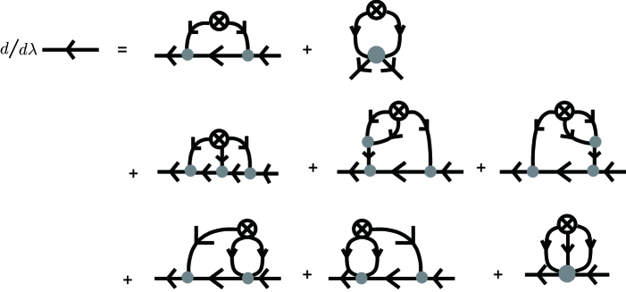
Figure 2: RG equation diagram for the propagator.

For example, the four-point function can be written as

$$\frac{\delta^{4}W_{\lambda}}{\delta J_{a}\delta K_{b}\delta K_{c}\delta K_{d}}$$

$$=\int ds_{1}\cdots ds_{4}G_{ae,\lambda}(k_{1};\eta_{a},s_{1})G_{fb,\lambda}(k_{2};s_{2},\eta_{b})G_{gc,\lambda}(k_{3};s_{3},\eta_{c})G_{hd,\lambda}(k_{4};s_{4},\eta_{d})$$

$$\qquad\times\bigl{\{}-\int ds_{5}ds_{6}G_{ij,\lambda}(k_{1}-k_{2};s_{5},s_{6})$$

$$\qquad\qquad\qquad\times\Gamma^{(3)}_{\chi_{e}\varphi_{f}\varphi_{i}}(k_{1},s_{1};k_{2},s_{2};k_{1}-k_{2},s_{5})\Gamma^{(3)}_{\chi_{j}\varphi_{j}\varphi_{h}}(k_{1}-k_{2},s_{6};k_{3},s_{3};k_{4},s_{4})$$

$$\qquad\qquad+\Gamma^{(4)}_{\chi_{e}\varphi_{f}\varphi_{g}\varphi_{h}}(k_{1},s_{1};k_{2},s_{2};k_{3},s_{3};k_{4},s_{4})\bigr{\}}\delta(k_{1}-k_{2}-k_{3}-k_{4}).$$ (72)

In Fig.2, we have drawn the Feynman diagrams for the RG equation. The four-point function in the RG equation gives the first and second diagrams in Fig.2. Other diagrams in Fig.2 come from the five-point function

$$\frac{\delta^{5}W_{\lambda}}{\delta J_{a}\delta K_{b}\delta K_{c}\delta K_{d}\delta K_{e}}$$

$$=\int ds_{1}\cdots ds_{4}G_{af,\lambda}(k_{1};\eta_{a},s_{1})G_{gb,\lambda}(k_{2};s_{2},\eta_{b})G_{hc,\lambda}(k_{3};s_{3},\eta_{c})G_{id,\lambda}(k_{4};s_{4},\eta_{d})G_{je,\lambda}(k_{5};s_{5},\eta_{e})$$

$$\qquad\times\bigl{\{}\int ds_{6}ds_{7}ds_{8}ds_{9}G_{kl,\lambda}(k_{1}-k_{2};s_{6},s_{7})G_{mn,\lambda}(k_{5}+k_{4};s_{8},s_{9})\Gamma^{(3)}_{\chi_{f}\varphi_{g}\varphi_{k}}(k_{1},s_{1};k_{2},s_{2};k_{1}-k_{2},s_{6})$$

$$\qquad\qquad\qquad\times\Gamma^{(3)}_{\chi_{l}\varphi_{h}\varphi_{m}}(k_{1}-k_{2},s_{7};k_{3},s_{3};k_{5}+k_{4},s_{8})\Gamma^{(3)}_{\chi_{n}\varphi_{i}\varphi_{j}}(k_{5}+k_{4},s_{8};k_{4},s_{4};k_{5},s_{5})$$

$$\qquad\qquad\qquad\qquad\qquad\qquad\qquad\qquad\qquad\qquad\qquad\qquad\qquad\qquad+\cdots\bigr{\}}\delta(k_{1}-k_{2}-k_{3}-k_{4}-k_{5})\ ,$$ (73)

where we have explicitly displayed only the relevant one.

We can now calculate the RG equation. On the nonlinear scale, modes enter into the damping phase. Therefore, the nonlinear effect allows us to consider only the low wavenumber mode for the internal lines. Hence, we can take the large $k$ limit, where $k$ is the wavenumber of the renomalized propagator. In this paper, we approximate a solution by taking into account only the running of the 2-point function. We also ignore the propagation of the decaying mode. Thus, the coupling constant $\gamma_{abc}$ always appears in the following form:

$$\gamma({\bf k},{\bf p},{\bf q}) \equiv \hat{u}_{a}\gamma_{abc}({\bf k},{\bf p},{\bf q})u_{b}u_{c}$$ (74)

$$= \frac{1}{10p^{2}q^{2}}(6p^{2}q^{2}+5(p^{2}+q^{2}){\bf p}\cdot{\bf q}+4({\bf p}\cdot{\bf q})^{2})\ .$$

In the limit $p\gg q$, we obtain

$$\gamma({\bf k},{\bf p},{\bf q})\xrightarrow[p\gg q]{}\frac{{\bf p}\cdot{\bf q}}{2q^{2}}\ .$$ (75)

In our approximation, the diagrams we need to consider are the first, third, fourth and fifth ones in Fig.2. It is known that the fourth and fifth ones are higher order contributions than the third one Crocce:2005xz . The third one directly interacts with the initial conditions, so that all informations of the intial conditions transmit. From Eq.(74), we see the direct interaction linearly grows with the wavenumber ${\bf p}$. On the contrary, there are interactions outside the main path in the fourth and fifth diagrams. There, we can not take the limit $k\gg q$ and, hence, we cannot expect the linear growth. Thus, we can ignore them. As an additional approximation, we replace the propagator in the right hand side of the RG equation in Fig.2 with its linear expression.

Using the above aproximations, we can get the RG eqation for the propagator,

$$\partial_{\lambda}G_{ab,\lambda}(k;\eta_{a},\eta_{b})$$

$$=g_{ab}(\eta_{a},\eta_{b})\biggl{\{}2^{2}(2\pi)^{3}\int^{\eta_{a}}_{\eta_{b}}\!\!\!\!ds_{2}\int^{s_{2}}_{\eta_{b}}\!\!\!\!ds_{1}\exp(s_{1}+s_{2})$$

$$\qquad\qquad\qquad\qquad\times\int d^{3}{\bf q}\partial_{\lambda}P_{cd,\lambda}(q)\hat{u}_{c}\hat{u}_{d}\gamma({\bf k},{\bf q},{\bf k}-{\bf q})\gamma({\bf k}-{\bf q},-{\bf q},{\bf k})$$

$$\qquad\qquad\qquad\qquad-2^{3}(2\pi)^{3}\int^{\eta_{a}}_{\eta_{b}}\!\!\!\!ds_{3}\int^{s_{3}}_{\eta_{b}}\!\!\!\!ds_{2}\int^{s_{2}}_{\eta_{b}}\!\!\!\!ds_{1}\exp(s_{1}+s_{2}+s_{3})$$

$$\qquad\qquad\qquad\qquad\qquad\times\int d^{3}{\bf q_{1}}d^{3}{\bf q_{2}}d^{3}{\bf q_{3}}\partial_{\lambda}B_{cde,\lambda}({\bf q_{1}},{\bf q_{2}},{\bf q_{3}})\hat{u}_{c}\hat{u}_{d}\hat{u}_{e}$$

$$\qquad\qquad\qquad\qquad\qquad\quad\times\gamma({\bf k},{\bf q_{1}},{\bf k}-{\bf q_{1}})\gamma({\bf k}-{\bf q_{1}},{\bf k}+{\bf q_{3}},{\bf q_{2}})\gamma({\bf k}+{\bf q_{3}},{\bf q_{3}},{\bf k})\biggr{\}}$$

$$=g_{ab}(\eta_{a},\eta_{b})\biggl{\{}2\left(\exp(\eta_{a})-\exp(\eta_{b})\right)^{2}\partial_{\lambda}F_{P,\lambda}[k]-8\left(\exp(\eta_{a})-\exp(\eta_{b})\right)^{3}\partial_{\lambda}F_{B,\lambda}[k]\biggr{\}}\ ,$$ (76)

where we have defined

$$F_{P,\lambda}[k] \equiv (2\pi)^{3}\int d^{3}{\bf q}P_{cd,\lambda}(q)\hat{u}_{c}\hat{u}_{d}\gamma({\bf k},{\bf q},{\bf k}-{\bf q})\gamma({\bf k}-{\bf q},-{\bf q},{\bf k})$$ (77)

$$= (2\pi)^{3}\frac{\pi}{50}\int dqP_{cd,\lambda}(q)\hat{u}_{c}\hat{u}_{d}\biggl{(}3\frac{k^{4}}{q^{2}}-\frac{121}{6}k^{2}+9q^{2}-\frac{9}{2}\frac{q^{4}}{k^{2}}$$

$$\qquad\qquad\qquad+\left(-\frac{3}{2}\frac{k^{5}}{q^{3}}+\frac{9}{4}\frac{k^{3}}{q}+\frac{9}{4}kq-\frac{21}{4}\frac{q^{3}}{k}+\frac{9}{4}\frac{q^{5}}{k^{3}}\right)\log\left|\frac{k+q}{k-q}\right|\biggr{)}$$

and

$$F_{B,\lambda}[k] \equiv (2\pi)^{3}\int d^{3}{\bf q_{1}}d^{3}{\bf q_{2}}d^{3}{\bf q_{3}}B_{cde,\lambda}({\bf q_{1}},{\bf q_{2}},{\bf q_{3}})\hat{u}_{c}\hat{u}_{d}\hat{u}_{e}$$ (78)

$$\qquad\qquad\quad\times\gamma({\bf k},{\bf q_{1}},{\bf k}-{\bf q_{1}})\gamma({\bf k}-{\bf q_{1}},{\bf k}+{\bf q_{3}},{\bf q_{2}})\gamma({\bf k}+{\bf q_{3}},{\bf q_{3}},{\bf k}).$$

Here, we promote the linear propagator to the full nonlinear one following Mataresse and Pietroni Matarrese:2007wc . Solving the differential equation (76) with the initial condition $G_{ab,\lambda=0}=g_{ab}$ and taking the limit $\lambda$ goes to infinity, we obtain

$$G_{ab}(k;\eta_{a},\eta_{b})=g_{ab}(k;\eta_{a},\eta_{b})$$

$$\qquad\times\exp\Bigl{\{}2\left(\exp(\eta_{a})-\exp(\eta_{b})\right)^{2}F_{P}[k]-8\left(\exp(\eta_{a})-\exp(\eta_{b})\right)^{3}F_{B}[k]\Bigr{\}}$$ (79)

As a concrete example, we consider the model

$$\varphi_{0}({\bf x})=\varphi_{g}({\bf x})+\xi_{NL}(\varphi_{g}^{2}({\bf x})-\langle\varphi_{g}^{2}\rangle),$$ (80)

where $\varphi_{g}({\bf x})$ is a Gaussian field. It should be noted that this $\xi_{NL}$ is different from $f_{NL}$, because we are considering $\varphi_{a}$ instead of the curvature perturbation $\Phi$. Then the initial bispectrum $B_{abc}$ is written as

$$B_{abc}({\bf q_{a}},{\bf q_{b}},{\bf q_{c}})=2\xi_{NL}\delta({\bf q_{a}}+{\bf q_{b}}+{\bf q_{c}})(P(q_{a})P(q_{b})+P(q_{b})P(q_{c})+P(q_{c})P(q_{a})),$$ (81)

where $P(q)=P_{cd}(q)\hat{u}_{c}\hat{u}_{d}$. In the $k\gg p$ limit, we can deduce

$$F_{P}[k]\xrightarrow[k\gg q]{}-(2\pi)^{3}\frac{\pi k^{2}}{3}\int dqP_{cd}(q)\ ,$$ (82)

and

$$F_{B}[k]\xrightarrow[k\gg q]{}(2\pi)^{3}\frac{7}{80}\int d^{3}q_{1}d^{3}q_{2}d^{3}q_{3}$$

$$\qquad\qquad\qquad\qquad\times\left(\frac{({\bf k}\cdot{\bf q_{1}})({\bf k}\cdot{\bf q_{2}})}{q_{1}^{2}q_{2}^{2}}+\frac{({\bf k}\cdot{\bf q_{2}})({\bf k}\cdot{\bf q_{3}})}{q_{2}^{2}q_{3}^{2}}+\frac{({\bf k}\cdot{\bf q_{3}})({\bf k}\cdot{\bf q_{1}})}{q_{3}^{2}q_{1}^{2}}\right)B({\bf q}_{1},{\bf q}_{2},{\bf q}_{3})\ ,$$ (83)

where we have defined $B(q)=B_{cde}(q)\hat{u}_{c}\hat{u}_{d}\hat{u}_{e}$.

From the shape of the CDM spectrum, we can estimate the scale where the running of the propagator is important. The nonlinear effect works when the argument of exponential in Eq.(79) becomes ${\cal O}(1)$. The threshold for the power spectrum ($F_{P}a_{0}^{2}$) becomes $k\sim 0.1(1+z)\mbox{Mpc}^{-1}$. On the other hand, the threshold for the bispectrum ($F_{B}a_{0}^{2}$) is given by $k\sim 0.03\xi_{NL}^{-{1\over 2}}(1+z)^{3/2}\mbox{Mpc}^{-1}$. This means that, if the statistics is positively skewed and $\xi_{NL}>O(1)$, the effect of the initial bispectrum is a dominant one at present in the non-linear propagator. On the other hand, the negatively skewed non-Gaussianity delays the time each comoving mode enters the nonlinear regime. The above arguments imply that the non-Gaussianiy significantly affects the running of the propagator.

The propagator can be regarded as the measure of the memory of initial conditions. Only in the case the memory is left in the data, we can detect the primordial non-Gaussianity. According to the behavior of the nonlinear propagator, the modes in the range $k>0.1(1+z)\mbox{Mpc}^{-1}$ or $k>0.03\xi_{NL}^{-{1\over 2}}(1+z)^{3/2}\mbox{Mpc}^{-1}$ seems to have already lost the memory to the initial conditions. This means that, at the time $z\sim 1$, we can not observe the primordial non-Gaussianity around the scale $k=1\mbox{Mpc}^{-1}$. In order to investigate the primordial non-Gausianity at the comoving scale $1\mbox{Mpc}$, we have to look at the Universe at $z>10$. One possibility is the observation of $21\mbox{cm}$ line. As to this, many observational projects, such as the Low Frequency Array (LOFAR), the Square Kilometer Array (SKA), the Mileura Widefield Array (MWA) and the $21\mbox{cm}$ array (21CMA), are ongoing or being planed Furlanetto:2006jb .

V Conclusion

We have studied the Newtonian cosmological perturbation theory from the field theoretical point of view. We have extended the renomalization group method proposed by Mataresse and Pietroni to the case of a primordial non-Gaussian density fluctuations. In particular, we have obtained the generating functional for the cosmic evolution of fluctuations with non-Gaussian statistics. As an application, we have calculated the nonlinear propagator and examined how the non-Gaussianity affects the memory of cosmic fields to their initial conditions. It turned out that the initial non-Gaussianity affects on the running of the propagator. For the positively skewed case, the nonlinearity starts at ealier stage. In the opposite case, the nonlinearity is postpond compared with the Gaussian case.

Assuming the ${\cal O}(1)$ positively skewed non-Gaussianity, we can conclude that the nonlinear propagator damps in the range $k>0.1(1+z)\mbox{Mpc}^{-1}$ or $k>0.03\xi_{NL}^{-{1\over 2}}(1+z)^{3/2}\mbox{Mpc}^{-1}$. Hence, if we want to investigate the initial non-gaussianity at the scale $k>1\mbox{Mpc}^{-1}$, the observation at $z>10$ is required. One interesting possibility is to observe fluctuations of $21\mbox{cm}$ absorption line in the cosmic maicrowave background radiation. In the negatively skewed case, the effect is opposite. Therefore, the time entering the nonlinear scale is postponed for the mode with a fixed comoving wavenumber.

As an application of our formalism, we can estimate the effect of the primordial non-Gaussianity on the BAO. More intriguingly, we can calculate the bispectrum of cosmic fields which provide a more clear test of non-Gaussianity. It is also intriguing to calculate BAO feature in the bispectrum. Again, the bispectrum of 21 cm line fluctuations is an interesting target.

Recent observational progress allows us to know the large scale structure at high redshift. It should be emphasized that the field theoretical approach gives a simple way to calculate correlation functions with different times. Therefore, the field theoretical method in cosmology deserves further investigations.

References

• (1) V. Sahni and P. Coles, Phys. Rept.  262, 1 (1995) [arXiv:astro-ph/9505005].
• (2) F. Bernardeau, S. Colombi, E. Gaztanaga and R. Scoccimarro, Phys. Rept.  367, 1 (2002) [arXiv:astro-ph/0112551].
• (3) Y. Suto and M. Sasaki, Phys. Rev. Lett.  66, 264 (1991).
• (4) N. Makino, M. Sasaki and Y. Suto, Phys. Rev.  D 46, 585 (1992).
• (5) B. Jain and E. Bertschinger, Astrophys. J.  431, 495 (1994) [arXiv:astro-ph/9311070].
• (6) R. Scoccimarro and J. Frieman, Astrophys. J. Suppl.  105, 37 (1996) [arXiv:astro-ph/9509047].
• (7) T. Matsubara, arXiv:astro-ph/0006269.
• (8) M. Crocce and R. Scoccimarro, Phys. Rev.  D 73, 063519 (2006) [arXiv:astro-ph/0509418].
• (9) P. McDonald, Phys. Rev.  D 75, 043514 (2007) [arXiv:astro-ph/0606028].
• (10) N. Afshordi, Phys. Rev.  D 75, 021302 (2007) [arXiv:astro-ph/0610336].
• (11) S. Matarrese and M. Pietroni, arXiv:astro-ph/0702653.
• (12) S. Matarrese and M. Pietroni, arXiv:astro-ph/0703563.
• (13) D. J. Eisenstein et al. [SDSS Collaboration], Astrophys. J.  633, 560 (2005) [arXiv:astro-ph/0501171].
• (14) E. Huff, A. E. Schulz, M. White, D. J. Schlegel and M. S. Warren, Astropart. Phys.  26, 351 (2007) [arXiv:astro-ph/0607061].
• (15) D. Jeong and E. Komatsu, Astrophys. J.  651, 619 (2006) [arXiv:astro-ph/0604075].
• (16) M. Crocce and R. Scoccimarro, arXiv:0704.2783 [astro-ph].
• (17) T. Nishimichi et al., arXiv:0705.1589 [astro-ph].
• (18) M. Crocce and R. Scoccimarro, Phys. Rev.  D 73, 063520 (2006) [arXiv:astro-ph/0509419].
• (19) P. Valageas, arXiv:astro-ph/0611849.
• (20) E. Komatsu et al. [WMAP Collaboration], Astrophys. J. Suppl.  148, 119 (2003) [arXiv:astro-ph/0302223].
• (21) N. Bartolo, E. Komatsu, S. Matarrese and A. Riotto, Phys. Rept.  402, 103 (2004) [arXiv:astro-ph/0406398].
• (22) K. Koyama, J. Soda and A. Taruya, Mon. Not. Roy. Astron. Soc.  310, 1111 (1999) [arXiv:astro-ph/9903027].
• (23) J. A. Willick, arXiv:astro-ph/9904367.
• (24) J. Robinson, E. Gawiser and J. Silk, Astrophys. J.  532, 1 (2000) [arXiv:astro-ph/9906156].
• (25) S. Matarrese, L. Verde and R. Jimenez, Astrophys. J.  541, 10 (2000) [arXiv:astro-ph/0001366].
• (26) R. Scoccimarro, arXiv:astro-ph/0002037.
• (27) N. Seto, arXiv:astro-ph/0102195.
• (28) R. Scoccimarro, E. Sefusatti and M. Zaldarriaga, Phys. Rev.  D 69, 103513 (2004) [arXiv:astro-ph/0312286].
• (29) C. Hikage, E. Komatsu and T. Matsubara, Astrophys. J.  653, 11 (2006) [arXiv:astro-ph/0607284].
• (30) E. Sefusatti, C. Vale, K. Kadota and J. Frieman, arXiv:astro-ph/0609124.
• (31) S. Furlanetto, S. P. Oh and F. Briggs, Phys. Rept.  433, 181 (2006) [arXiv:astro-ph/0608032].