On Colorings of Squares of Outerplanar Graphs

Abstract

We study vertex colorings of the square $G^{2}$ of an outerplanar graph $G$. We find the optimal bound of the inductiveness, chromatic number and the clique number of $G^{2}$ as a function of the maximum degree $\Delta$ of $G$ for all $\Delta\in\mbox{$\mathbb{N}$}$. As a bonus, we obtain the optimal bound of the choosability (or the list-chromatic number) of $G^{2}$ when $\Delta\geq 7$. In the case of chordal outerplanar graphs, we classify exactly which graphs have parameters exceeding the absolute minimum.

2000 MSC: 05C05, 05C12, 05C15.

Keywords: outerplanar, chordal, weak dual, power of a graph, greedy coloring, chromatic number, clique number, inductiveness.

1 Introduction

The square of a graph $G$ is the graph $G^{2}$ on the same vertex set with edges between pair of vertices of distance one or two in $G$. Coloring squares of graphs has been studied, e.g., in relation to frequency allocation. This models the case when nodes represent both senders and receivers, and two senders with a common neighbor will interfere if using the same frequency.

The problem of coloring squares of graphs has particularly seen much attention on planar graphs. A conjecture of Wegner [12] dating from 1977 (see [8]), states that the square of every planar graph $G$ of maximum degree $\Delta\geq 8$ has a chromatic number which does not exceed $3\Delta/2+1$. The conjecture matches the maximum clique number of these graphs. Currently the best upper bound known is $1.66\Delta+78$ by Molloy and Salavatipour [11].

An earlier paper of the current authors [1] gave a bound of $\lceil 1.8\Delta\rceil$ for the chromatic number of squares of planar graph with large maximum degree $\Delta\geq 749$. This is based on bounding the inductiveness of the graph, which is the maximum over all subgraphs $H$ of the minimum degree of $H$. It was also shown there that this was the best possible bound on the inductiveness. Borodin et al [4] showed that this bound holds for all $\Delta\geq 48$. Inductiveness has the additional advantage of also bounding the list-chromatic number.

Inductiveness leads to a natural greedy algorithm (henceforth called Greedy): Select vertex $u\in V(G)$ of minimum degree, sometimes called a simplicial vertex of $G$, recursively color $G\setminus u$, and finally color $u$ with the smallest available color. Alternatively, $k$-inductiveness leads to an inductive ordering $u_{1},u_{2},\ldots,u_{n}$ of the vertices such that any vertex $u_{i}$ has at most $k$ neighbors among $\{u_{i+1},\ldots,u_{n}\}$. Then, if we color the vertices first-fit in the reverse order $u_{n},u_{n-1},\ldots,u_{1}$ (i.e. assigning each vertex the smallest color not used among its previously colored neighbors), the number of colors used is at most $k+1$. Implemented efficiently, the algorithm runs in time linear in the size of the graph [7]. The algorithm has also the special advantage that it requires only the square graph $G^{2}$ and does not require information about the underlying graph $G$.

The purpose of this article is to further contribute to the study of various vertex colorings of squares of planar graphs, by examining an important subclass of them, the class of outerplanar graphs. Observe that the neighborhood of a vertex with $\Delta$ neighbors induces a clique in the square graph. Thus, the chromatic number, and in fact the clique number, of any graph of maximum degree $\Delta$ is necessarily a function of $\Delta$ and always at least $\Delta+1$.

Our results.

We derive tight bounds on chromatic number, as well as the inductiveness and the clique number of the square of an outerplanar graph $G$ as a function of the maximum degree $\Delta$ of $G$. One of the main results, given in Section 3, is that when $\Delta\geq 7$, the inductiveness of $G^{2}$ is exactly $\Delta$. It follows that the clique and chromatic numbers are exactly $\Delta+1$ and that Greedy yields an optimal coloring. As a bonus we obtain in this case that the choosability (see Definition 3.11) is the optimal $\Delta+1$. We can then treat the low-degree cases separately to derive a linear-time algorithm independent of $\Delta$. We examine in detail the low-degree cases, $\Delta<7$, and derive best possible upper bounds on the maximum clique and chromatic numbers, as well as inductiveness of squares of outerplanar graphs. These bounds are illustrated in Table LABEL:tab:Delta. We treat the special case of chordal outerplanar graphs separately, and further classify all chordal outerplanar graphs $G$ for which the inductiveness of $G^{2}$ exceeds $\Delta$ or the clique or chromatic number of $G^{2}$ exceed $\Delta+1$.

	Chordal			General
$\Delta$	$\omega$	ind	$\chi$	$\omega$	ind	$\chi$
2	$\Delta+1$	$\Delta$	$\Delta+1$	$\Delta+3$	$\Delta+2$	$\Delta+3$
3	$\Delta+1$	$\Delta$	$\Delta+1$	$\Delta+2$	$\Delta+1$	$\Delta+2$
4	$\Delta+2$	$\Delta+1$	$\Delta+2$	$\Delta+2$	$\Delta+2$	$\Delta+2$
5	$\Delta+1$	$\Delta+1$	$\Delta+1$	$\Delta+1$	$\Delta+1$	$\Delta+2$
6	$\Delta+1$	$\Delta+1$	$\Delta+1$	$\Delta+1$	$\Delta+1$	$\Delta+1$
7+	$\Delta+1$	$\Delta$	$\Delta+1$	$\Delta+1$	$\Delta$	$\Delta+1$

Table 1: Optimal upper bounds for the clique number, inductiveness, and chromatic number of the square of a chordal / non-chordal outerplanar graph $G$.

Related results.

It is straightforward to show that the inductiveness of a square graph of an outerplanar graph of degree $\Delta$ is at most $2\Delta$ (see [1]), and this is attained by an inductive ordering of $G$. Calamoneri and Petreschi [5] gave a linear time algorithm to distance-2 color outerplanar graphs, as well as for related problems. They showed that it uses an optimal $\Delta+1$ colors whenever $\Delta\geq 7$, and at most $\Delta+2$ colors for $\Delta\geq 4$. In comparison, we give tight upper and lower bounds for all values of $\Delta$, give a thorough treatment of the subclass of chordal graphs, and analyze a generic parameter, inductiveness, that gives as a bonus similar bounds for the list chromatic number.

Zhou, Kanari and Nishizeki [14] gave a polynomial time algorithm to find an optimal coloring of any power of a partial $k$-tree $G$, given $G$. Since outerplanar graphs are partial 2-trees, this solves the coloring problem we consider. For squares of outerplanar graphs, their algorithm has complexity $O(n(\Delta+1)^{2^{37}}+n^{3})$, which is impractical for any values of $\Delta$ and $n$. When $\Delta$ is constant, one can use the observation of Krumke, Marathe and Ravi [9] that squares of outerplanar graphs have treewidth at most $k\leq 3\Delta-1$. Thus, one can use efficient ($2^{O(k)}n$ time) algorithms for coloring partial $k$-trees, obtaining a linear-time algorithm when $\Delta$ is constant.

Organization.

The rest of the paper is organized as follows: In Section 2 we introduce our notation and definitions, and show how the problems regarding the clique number and chromatic number reduce to the case of biconnected outerplanar graphs. Inductiveness is treated in Section 3. We then treat the chordal case in Section 4. Many examples here show that the lower bounds derived in other sections (i.e. Sections 3 and 5) are optimal. The clique number is derived in Section 5. The last Section 6 derives optimal bounds on chromatic number in each of the smaller cases of $\Delta\in\{2,3,4,5,6\}$. The main result there is the optimal bound for the chromatic number of $G^{2}$ in the hardest case when $\Delta=6$.

2 Definitions

In this section we give some basic definitions and prove results that will be used later for our results in the following sections.

Graph notation.

The set $\{1,2,3,\ldots\}$ of natural numbers will be denoted by $\mathbb{N}$. Unless otherwise stated, a graph $G$ will always be a simple graph $G=(V,E)$ where $V=V(G)$ is the set of vertices or nodes, and $E=E(G)$ the set of edges of $G$. The edge between the vertices $u$ and $v$ will be denoted by $uv$ (here $uv$ and $vu$ will mean the same undirected edge). By coloring we will always mean vertex coloring. We denote by $\chi(G)$ the chromatic number of $G$ and by $\omega(G)$ the clique number of $G$. The degree of a vertex $u$ in graph $G$ is denoted by $d_{G}(u)$. We let $\delta(G)$ and $\Delta(G)$ denote the minimum and maximum degree of a vertex in $G$ respectively. When there is no danger of ambiguity, we simply write $\Delta$ instead of $\Delta(G)$. We denote by $N_{G}(u)$ the open neighborhood of $u$ in $G$, that is the set of all neighbors of $u$ in $G$, and by $N_{G}[u]$ the closed neighborhood of $u$ in $G$, that additionally includes $u$.

The square graph $G^{2}$ of a graph $G$ is a graph on the same vertex set as $G$ in which additionally to the edges of $G$, every two vertices with a common neighbor in $G$ are also connected with an edge. Clearly this is the same as the graph on $V(G)$ in which each pair of vertices of distance 2 or less in $G$ are connected by an edge in $G^{2}$.

By a $k$-vertex we will mean a vertex of degree at most 2 in $G$ and distance-2 degree at most $k$. ‘

Tree terminology.

The diameter of $T$ is the number of edges in the longest simple path in $T$ and will be denoted by $\mbox{\rm diam}(T)$. For a tree $T$ with $\mbox{\rm diam}(T)\geq 1$ we can form the pruned tree $\mbox{\rm pr}(T)$ by removing all the leaves of $T$. A center of $T$ is a vertex of distance at most $\lceil\mbox{\rm diam}(T)/2\rceil$ from all other vertices of $T$. A center of $T$ is either unique or one of two unique adjacent vertices. When $T$ is rooted at $r\in V(T)$, the $k$-th ancestor, if it exists, of a vertex $u$ is the vertex on the unique path from $u$ to $r$ of distance $k$ from $u$. An ancestor of $u$ is a $k$-th ancestor of $u$ for some $k\geq 0$. Note that $u$ is viewed as an ancestor of itself. The parent (grandparent) of a vertex is then the $1$-st ($2$-nd) ancestor of the vertex. The sibling of a vertex is another child of its parent, and a cousin is child of a sibling of its parent. The height of a rooted tree is the length of the longest path from the root to a leaf. The height of a vertex $u$ in a rooted tree $T$ is the height of the rooted subtree of $T$ induced by all vertices with $u$ as an ancestor. A tree is said to be full if it contains no degree-two vertices.

Note that in a rooted tree $T$, vertices of height zero are the leaves (provided that the root is not a leaf). Vertices of height one are the parents of leaves, that is, the leaves of the pruned tree $\mbox{\rm pr}(T)$ and so on. In general, for $k\geq 0$ let $\mbox{\rm pr}^{k}(T)$ be given recursively by $\mbox{\rm pr}^{0}(T)=T$ and $\mbox{\rm pr}^{k}(T)=\mbox{\rm pr}(\mbox{\rm pr}^{k-1}(T))$. Clearly $V(T)\supset V(\mbox{\rm pr}(T))\supset\cdots\supset V(\mbox{\rm pr}^{k}(T))\supset\cdots$ is a strict inclusion. With this in mind we have an alternative “root-free” description of the height of vertices in a tree.

Observation 2.1

Let $T$ be a tree and $0\leq k\leq\lfloor\mbox{\rm diam}(T)/2\rfloor$. The vertices of height $k$ in $T$ are precisely the leaves of $\mbox{\rm pr}^{k}(T)$.

Inductiveness.

The inductiveness or the degeneracy of a graph $G$, denoted by $\mbox{\rm ind}(G)$, is the natural number defined by

$$\mbox{\rm ind}(G)=\max_{H\subseteq G}\left\{\delta(H)\right\},$$

where $H$ runs through all the induced subgraphs of $G$. If $k\geq\mbox{\rm ind}(G)$ then we say that $G$ is $k$-inductive.

In a graph $G$ of maximum degree at most $\Delta$, note that for any $u\in V(G)$, the vertex set $N_{G}[u]$ will induce a clique in $G^{2}$, and hence $\omega(G^{2}),\chi(G^{2})\geq\Delta+1$. Since $\mbox{\rm ind}(G^{2})+1\geq\chi(G^{2})$, the upper bound of $\mbox{\rm ind}(G)$ is necessarily an increasing function $f(\Delta)$ of $\Delta\in\mbox{$\mathbb{N}$}$. In general, the inductiveness of a graph $G$ yields an ordering $\{u_{1},u_{2},\ldots,u_{n}\}$ of the vertex set $V(G)$ of $G$, such that each vertex $u_{i}$ has at most $\mbox{\rm ind}(G)$ neighbors among the previous vertices $u_{1},\ldots,u_{i-1}$ that is to say $|N_{G}(u_{i})\cap\{u_{1},\ldots,u_{i-1}\}|\leq\mbox{\rm ind}(G)$. This gives us an efficient way to color every graph $G$ by at most $\mbox{\rm ind}(G)+1$ colors in a greedy fashion.

Biconnectivity.

The blocks of a graph $G$ are the maximal biconnected subgraphs of $G$. A cutvertex is a vertex shared by two or more blocks. A leaf block is a block with only one cutvertex (or none, if the graph is already biconnected).

We show here that we can assume, without loss of generality, that $G$ is biconnected when considering the chromatic number or the clique number of $G^{2}$: Let $G$ be a graph and $\mathcal{B}$ the set of its biconnected blocks. In the same way that $\omega(G)=\max_{B\in\mathcal{B}}\{\omega(B)\}$ and $\chi(G)=\max_{B\in\mathcal{B}}\{\chi(B)\}$, we have the following.

Lemma 2.2

For a graph $G$ with a maximum degree $\Delta$ and set $\mathcal{B}$ of biconnected blocks we have

$$\omega(G^{2}) = \max\{\max_{B\in\mathcal{B}}\{\omega(B^{2})\},\Delta+1\},$$

$$\chi(G^{2}) = \max\{\max_{B\in\mathcal{B}}\{\chi(B^{2})\},\Delta+1\}.$$

Further, optimal $\chi(B^{2})$-colorings of the squares of all the blocks $B^{2}$ can be modified to a $\chi(G^{2})$-coloring of $G^{2}$ in a greedy fashion.

• First note that a clique of $G^{2}$ with vertices contained in more than one block of $G$ must contain the cutvertex of two blocks. Therefore the clique must be induced by the closed neighborhood of this cutvertex, and hence of size at most $\Delta+1$. This proves the first formula for $\omega(G^{2})$.

  For the chromatic number of $G^{2}$, we proceed by induction on $b=|\mathcal{B}|$. The case $b=1$ is a tautology, so assume $G$ has $b\geq 2$ blocks and that the lemma is true for $b-1$. Let $B$ be a leaf block and let $G^{\prime}=\cup_{B^{\prime}\in\mathcal{B}\setminus\{B\}}B^{\prime}$, with $w=V(B)\cap V(G^{\prime})$ as a cutvertex. If $\Delta^{\prime}$ is the maximum degree of $G^{\prime}$, then by induction hypothesis $\chi(G^{\prime 2})=\max\{\max_{B^{\prime}\in\mathcal{B}\setminus\{B\}}\{\chi(B^{\prime 2})\},\Delta^{\prime}+1\}$. Assume we have a $\chi(G^{\prime 2})$-coloring of $G^{\prime 2}$ and a $\chi(B^{2})$-coloring of $B^{2}$, the latter given by a map $c_{B}:V(B)\rightarrow\{1,\ldots,\chi(B^{2})\}$. Since $w$ is a cutvertex we have a partition $N_{G}[w]=\{w\}\cup N_{B}\cup N_{G^{\prime}}$, where $N_{B}=N_{G}(w)\cap V(B)$ and $N_{G^{\prime}}=N_{G}(w)\cap V(G^{\prime})$. In the given coloring $c_{B}$ all the vertices in $N_{B}$ have received distinct colors, since they all have $w$ as a common neighbor in $B$. Since $|N_{G}[w]|\leq\Delta+1$ there is a permutation $\sigma$ of $\{1,\ldots,\max\{\chi(B^{2}),\Delta+1\}\}$ such that $\sigma\circ\mathbf{i}\circ c_{B}$ yields a new $\chi(B^{2})$-coloring of $B^{2}$ such that all vertices in $N_{G}[w]$ receive distinct colors (here $\mathbf{i}$ is the inclusion map of $\{1,\ldots,\chi(B^{2})\}$ in $\{1,\ldots,\max\{\chi(B^{2}),\Delta+1\}\}$.) This together with the given $\chi(G^{\prime 2})$-coloring of $G^{\prime 2}$ provides a vertex coloring of $G^{2}$ using at most $\max\{\max\{\chi(B^{2}),\Delta+1\},\chi(G^{\prime 2})\}\leq\max\{\max_{B\in\mathcal{B}}\{\chi(B^{2})\},\Delta+1\}$, which completes our proof.     $\sqcap$$\sqcup$

Note that Lemma 2.2 provides a way to extend distance-2 colorings of the blocks of $G$ to a distance-2 coloring of the whole of $G$. Thus, by Lemma 2.2 we can assume our graphs are biconnected, both when considering clique and chromatic numbers of $G^{2}$.

For the inductiveness of $G^{2}$, such an extension property as Lemma 2.2, to express $\mbox{\rm ind}(G^{2})$ directly in terms of $\Delta$ and the inductiveness of the blocks of $G$, is not as straightforward although it can be done. This is mainly because the simplicial vertex of a biconnected block could be a cut-vertex of the graph. We will consider this better in Section 3.

Duals of outerplanar graphs.

For our arguments to come we need a few properties about outerplanar graphs, the first of which is an easy exercise (See [13]).

Claim 2.3

Every biconnected outerplanar graph has at least two vertices of degree 2.

To analyze the inductiveness of an outerplanar graph $G$, it is useful to consider the weak dual of $G$, denoted by $T^{*}(G)$ and defined in the following:

Lemma 2.4

Let $G$ be an outerplanar graph with an embedding in the plane. Let $G^{*}$ be its geometrical dual, and let $u^{*}_{\infty}\in V(G^{*})$ be the vertex corresponding to the infinite face of $G$. Then the weak dual graph $T^{*}(G)=G^{*}-u^{*}_{\infty}$ is a forest which satisfies the following:

1. $T^{*}(G)$ is tree iff $G$ is biconnected.

2. $T^{*}(G)$ has maximum degree at most three, if $G$ is chordal.

Note that for a biconnected chordal graph $G$, there is a one-to-one correspondence $u\leftrightarrow u^{*}$ between the degree-2 vertices $u$ of $G$, and the leaves $u^{*}$ of $T^{*}(G)$.

• (Lemma 2.4) This follows easily by Claim 2.3 and induction on $n=|V(G)|$.     $\sqcap$$\sqcup$

Note that any biconnected chordal outerplanar graph on $n$ vertices can be constructed in the following way: Start with two vertices $v$ and $w$ and connect them with an edge. For $i=1$ to $n-2$, inductively connect a vertex $u_{i}$ to two endvertices of an edge which bounds the infinite face. Hence, after the $i$-th step, the vertex $u_{i}$ is of degree 2. Simultaneously we construct the weak dual tree $T^{*}(G)$ on the vertices $u_{1}^{*},\ldots,u_{n-2}^{*}$, by adding $u_{i}^{*}$ as a leaf to the vertex in $\{u_{1}^{*},\ldots,u_{i-1}^{*}\}$ corresponding to the face containing the two neighbors of $u_{i}$ after the $i$-th step. Hence, we have the following.

Observation 2.5

For a biconnected chordal outerplanar graph $G$, there are two vertices $v,w\in V(G)$ such that there is a bijection $V(G)\setminus\{v,w\}\rightarrow V(T^{*}(G))$, given by $u\mapsto u^{*}$, such that degree-2 vertices of $G$ correspond to leaves of $T^{*}(G)$. Further, successfully removing degree-2 vertices from $G$ will result in removing leaves from $T^{*}(G)$ in such a way that the mentioned correspondence will still hold between degree-2 vertices of the altered graph $G$ and the leaves of the altered tree.

By Lemma 2.4, $T^{*}(G)$ for a chordal graph $G$ is a tree of maximum degree 3, and hence each of its leaves has at most one sibling.

Note, however, that if $G$ is not chordal then the assignment $u\mapsto u^{*}$ is only surjective and not bijective. Both in the chordal and non-chordal case we will call the vertex $u^{*}$ the dual vertex of $u$. For the non-chordal case, such a construction can be done in a similar fashion, except that we inductively add a path of length $\geq 2$ instead of length exactly 2

Faces and dual leafs.

For an outerplanar plane graph $G$ two faces of $G$ are said to be adjoint (shortened as adj.) if they share a common vertex. A $k$-face is a face $f$ with $k$ vertices and $k$ edges. This will be denoted by $|f|=k$.

For a bounded face $f$ of $G$ the corresponding dual vertex of $T^{*}(G)$ will be denoted by $f^{*}$. Note for a chordal $G$ and if $f$ has two bounding edges bounding the infinite face then $f^{*}=u^{*}$, the dual vertex of $f$ from above. We will, however, speak interchangeably of a face $f$ and its corresponding dual vertex $f^{*}$ (or $u^{*}$ from above in the chordal case) from $T^{*}(G)$, when there is no danger of ambiguity, and we will apply standard forest/tree vocabulary to faces from the tree terminology given previously when each component from $T^{*}(G)$ is rooted at a center. A sib of a face $f$ is a sibling in $T^{*}(G)$ that is adjoint to $f$.

A face $f$ is $i$-strongly simplicial, or $i$-ss for short, if either $f$ is isolated (that is $G$ consists of $f$ alone), or $f$ is a leaf in $T^{*}(G)$ satisfying one of the following: (i) $i=0$, or (ii) the parent face of $f$ in $T^{*}(G)$ is $(i-1)$-ss in $\mbox{\rm pr}(T^{*}(G))$. Thus, e.g. all leafs are $0$-ss, while those leafs whose siblings have no children are also 1-ss.

3 Inductiveness

In this section we will derive optimal bounds on inductiveness. The following is the main result of this section.

Theorem 3.1

For an outerplanar graph $G$ of maximum degree $\Delta\geq 5$, we have $\mbox{\rm ind}(G^{2})\leq\Delta+1$. If further, $\Delta\geq 7$, then $\mbox{\rm ind}(G^{2})=\Delta$.

To bound the inductiveness, it is sufficient to show that there always exists a vertex that has both small degree and small distance-2 degree. Recall that a $k$-vertex is a vertex of degree at most 2 in $G$ and distance-2 degree at most $k$.

Lemma 3.2

Suppose any outerplanar graph of maximum degree $\Delta$ contains a $k$-vertex. Then, any outerplanar graph $G$ of maximum degree $\Delta$ satisfies $\mbox{\rm ind}(G^{2})\leq k$.

• We show this by induction on $|V(G)|$. Let $G$ be an outerplanar graph with a $k$-vertex $u$. We choose one incident edge $uv$ and form the contraction $G/uv$; this is the simple graph obtained from $G$ by contracting the edge $uv$ into a single vertex $v^{\prime}$ and keeping all edges that were incident on either $u$ or $v$ (deleting multiple copies). Formally, $G/uv$ has the vertex set $V(G/uv)=(V(G)\setminus\{u,v\})\cup\{v^{\prime}\}$ and edge set $E(G/uv)=E(G[V\setminus\{u,v\}])\cup\{v^{\prime}w:uw\in E(G)\mbox{ or }vw\in E(G)\}$. The set of distance-2 neighbors of $v^{\prime}$ in $G/uv$ properly contains the set of distance-2 neighbors of $v$ in $G$. Hence, a $k$-inductive ordering of $(G/uv)^{2}$ also gives a $k$-inductive ordering of $G^{2}$ excluding $u$ and where $v$ is replaced with $v^{\prime}$. Further, since $u$ was of degree at most 2, the degree of $v^{\prime}$ is at most that of $v$, and hence the maximum degree of $G/uv$ is at most that of $G$. By induction, there is such a $k$-inductive ordering of $(G/uv)^{2}$. By prepending $u$ to that ordering, replacing $v^{\prime}$ by $v$, we obtain a $k$-inductive ordering of $G^{2}$.     $\sqcap$$\sqcup$

Recall that a leaf block $B$ of $G$ contains just one cutvertex. Call a block $B$ simple if $\mbox{\rm diam}(T^{*}(B))\leq 2$, that is, $T^{*}(B)$ is empty, a single vertex, a single edge, or a star on three or more vertices.

Lemma 3.3

Any simple leaf block contains a $(\Delta+1)$-vertex of $G$ if $\Delta\geq 5$ and a $\Delta$-vertex if $\Delta\geq 6$.

• If $B$ is a single edge, then the leaf node is a $\Delta$-vertex. If $B$ is a 3-cycle, then either of the non-cut-vertices are $\Delta$-vertices. When $B$ is a $k$-cycle, for $k\geq 4$, then any node on the cycle that is not adjacent to the cut vertex is a $4$-vertex.

  Assume now that $T^{*}(B)$ is a single edge or a star on $\geq 3$ vertices. Clearly we have $\Delta(B)\leq 4$. If $B$ contains a degree-2 vertex $v$ of distance 2 or more from the cutvertex, then $v$ is a 6-vertex. So $v$ is a $(\Delta+1)$-vertex if $\Delta\geq 5$ and $\Delta$-vertex if $\Delta\geq 6$. If all the degree-2 vertices of $B$ are adjacent to the cutvertex of $G$, then $B$ is a diagonalized $C_{k}$ where $k\in\{4,5\}$. In this case both the degree-2 vertices of $B$ are $\Delta$-vertices of $G$. Hence we have the lemma.     $\sqcap$$\sqcup$

By Lemma 3.3 we will focus on non-simple leaf blocks for the rest of this section.

We start our search for a $k$-vertex at a face that has some nice properties. Recall the definition of a $i$-ss face. Notice that a face is $1$-ss iff its parent in $T^{*}(G)$ has no grandchildren, while it is $2$-ss if it either has no grandparent in $T^{*}(G)$, or if its grandparent is not the 3-rd ancestor of another face. Note that if $B$ is not simple, then for any rooting of $T^{*}(B)$ there are always faces with parents and grandparents.

Lemma 3.4

Let $B$ be a non-simple leaf block of $G$ and let $i$ be a non-negative integer. Then, $B$ contains an $i$-ss face $f$, its parent $f^{\prime}$, its grandparent $f^{\prime\prime}$ and an edge $e$ on the boundary of $f^{\prime\prime}$, such that $e$ separates $f^{\prime\prime}$ and all its descendants (its children and grandchildren) from the rest of $G$.

• If $G=B$ is biconnected let $r$ be any face. Otherwise, if $G\neq B$, let $r$ be any face that contains the cutvertex on its boundary and an edge bounding the infinite face. Let $T^{*}(B)$ be rooted at $r$ and let $f$ be a face of maximum distance from $r$ in $T^{*}(B)$. It is not hard to see that the center(s) of $T^{*}(B)$ is(are) on the path from $f$ to $r$, and hence $f$ is an endvertex of a maximum length path of $T^{*}(B)$. By definition of $i$-ss, $f$ is therefore $i$-ss for any $i\geq 0$. Also, $f$ has a parent $f^{\prime}$ and a grandparent $f^{\prime\prime}$.

  If $f$ has a great-grandparent $f^{\prime\prime\prime}$, then we let $e$ be the edge that separates $f^{\prime\prime}$ from $f^{\prime\prime\prime}$ in $T^{*}(B)$. This edge separates $f^{\prime\prime}$ and all its descendants from the rest of $B$, including $r$ and thus necessarily also from the rest of $G$.

  If $f$ has no great-grandparent, then $r=f^{\prime\prime}$ and we let $e$ be an edge incident on the cutvertex and the infinite face.     $\sqcap$$\sqcup$

Claim 3.5

Assume that we have faces $f$, $f^{\prime}$ and $f^{\prime\prime}$ in a block $B$ of $G$ as promised by Lemma 3.4.

1. If $ab$ is the edge separating $f^{\prime}$ from $f^{\prime\prime}$, then either $a$ or $b$ has degree at most 6 in $G$.

2. If $cd$ is the edge separating $f$ from $f^{\prime}$, then either $c$ or $d$ has degree at most 4 in $G$.

• Note that the cutvertex is either neither of the endvertices of the edge $e$ that separates $f^{\prime\prime}$ and all its descendants from the rest of $G$, or one of them.

  The first statement is true since $f$ is 2-ss in the block $B$, and the second statement is true since $f$ is 1-ss in $B$.     $\sqcap$$\sqcup$

Reducible configurations.

A configuration is an induced plane subgraph with certain vertices specially marked as having no neighbors outside the subgraph. A configuration is $k$-reducible for an integer $k$, if there exists a $k$-vertex for it. When $k$ is understood, we shall simply speak of a reducible configuration.

We will give an exhaustive decision tree, or a flowchart, that leads to a reducible configuration: A $(\Delta+1)$-reducible one when $\Delta\geq 5$ in Figure 1(a), and $\Delta$-reducible when $\Delta\geq 7$ in Figure 1(b). Each of the boxes of the branches corresponds to one of the reducible configurations of Figures 2-4, to be described shortly.

We shall assume that we are given $f$, $f^{\prime}$, and $ab$ as promised by Lemma 3.4. In the flowchart we use the following notation: Recall that the cardinality of a face $f$, denoted $|f|$, is its number of vertices. $f$ is incident on $ab$ if it contains one of its vertices. We shall assume that if $f$ is incident on one of the vertices of $ab$, then that vertex will be named $b$. When traversing the flowchart (either one in Figure 1), we shall assume that all sibs of a face are tested for a Y branch before proceeding to the corresponding N branch.

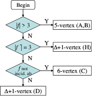
(a) $(\Delta+1)$-inductiveness, $\Delta\geq 5$

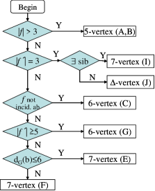
(b) $\Delta$-inductiveness, $\Delta\geq 7$

Figure 1: Reduction flowcharts

Each of the subfigures (A)-(J) in Figures 2-4 gives a configuration with a $k$-vertex marked as $u$. Each of them expresses more generally a collection of configurations, allowing for optional vertices as well as symmetric translations. Edges that lie on the infinite face are shown in bold, while internal edges are thin. Optional vertices and edges are shown with dotted edges. Vertices shown in white have possible additional edges, while all neighbors of dark vertices (in blue) are shown in the figure. We mark an $i$-ss face $f$ in the figure, along with its parent $f^{\prime}$.

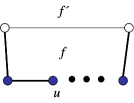
A $|f|\geq 5\Rightarrow$ 4-vertex

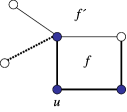
B $|f|=4\Rightarrow$ 5-vertex

Figure 2: Configurations for the case $|f|\geq 4$

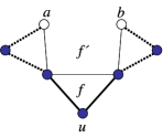
C $|f|=3$, $|f^{\prime}|\geq 4$, $f$ not incid. on $ab$ $\Rightarrow$ 6-vertex

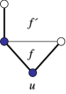
D $|f|=3$, sib missing $\Rightarrow$ $(\Delta+1)$-vertex

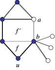
E $|f|=3$, $|f^{\prime}|=4$, all children of $f^{\prime}$ incid. on $ab$, $d_{G}(b)\leq 6$ $\Rightarrow$ $7$-vertex

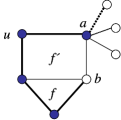
F $|f|=3$, $|f^{\prime}|=4$, no sib, $d_{G}(a)\leq 5$ $\Rightarrow$ $7$-vertex

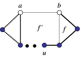
G $|f|=3$, $|f^{\prime}|\geq 5$, all children of $f^{\prime}$ incid. on $ab$ $\Rightarrow$ $6$-vertex

Figure 3: Configurations for the case $|f|=3$ and $|f^{\prime}|\geq 4$

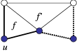
H $|f|=|f^{\prime}|=3\Rightarrow(\Delta+1)$-vertex

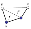
I $|f|=|f^{\prime}|=3$, $\nexists\mbox{sib}\Rightarrow\Delta$-vertex

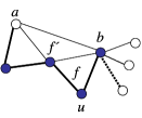
J $|f|=|f^{\prime}|=3,\mbox{$\exists$ sib}\Rightarrow 7$-vertex

Figure 4: Configurations for the case $|f|=|f^{\prime}|=3$

A set of configurations is unavoidable for a class of graphs if every graph in the class contains at least one configuration from the set. Our main technique, that bears a slight resemblance to the four color theorem [3], is to give an unavoidable set of reducible configurations.

For reductions (B), (C), (D), (G), (H), and (I) to apply, $f$ must be 1-ss, while for (E), (F), or (J) to apply, $f$ must be 2-ss.

Lemma 3.6

$\{A,B,C,D,H\}$ from Figures 2-4 is an unavoidable set of $(\Delta+1)$-configurations, for the class of outerplanar graphs of maximum degree $\Delta\geq 5$ with no simple leaf blocks.

• We basically go through the flowchart in Figure 1(a). Assume $f$, $f^{\prime}$, and $ab$ as promised by Lemma 3.4. If $|f|\geq 4$, then we have either case (A) or (B). Assume then that $|f|=3$ and consider its parent face $f^{\prime}$. If $|f^{\prime}|=3$, then we have case (H); otherwise, assume $|f^{\prime}|\geq 4$. If $f$ (or one of its sibs) is not incident on $ab$, then case (C) holds. Otherwise, $f$ is missing a sib on at least one side, so some edge of $f^{\prime}$ borders the infinite face, in which case (D) holds. In each case we obtain a $(\Delta+1)$-vertex and hence we have the lemma.     $\sqcap$$\sqcup$

From the above proof and Figure 1(a) we obtain the following.

Corollary 3.7

In each of the configurations from the unavoidable set $\{A,B,C,D,H\}$ in Lemma 3.6, our $(\Delta+1)$-vertex is on the boundary of the 1-ss face $f$.

We have similarly the following for $\Delta\geq 7$.

Lemma 3.8

$\{A,B,C,E,F,G,I,J\}$ from Figures 2-4 is an unavoidable set of $\Delta$-configurations, for the class of outerplanar graphs of maximum degree $\Delta\geq 7$ with no simple leaf blocks.

• We traverse the flowchart in Figure 1(b). Assume $f$, $f^{\prime}$, and $ab$ as promised by Lemma 3.4. If $|f|\geq 3$, then we have either of cases (A) and (B). Hence, we assume from now that $|f|=3$.

  Consider the case $|f^{\prime}|=3$. If $f$ has no sibling, then the case (I) applies and we have a $\Delta$-vertex. Otherwise, $f$ has a sibling, which we can (by the above) assume is also a 3-face. Since both $f$ and its sibling are 2-ss, then one of them is bounded by three vertices of degree 2, 4 and at most 6 in $G$. W.l.o.g. we may assume $f$ to be this very face, in which case (J) applies and we have a $7$-vertex.

  Consider now the case $|f^{\prime}|\geq 4$. If $f$ is not incident on $ab$, then the case (C) applies and we have a $6$-vertex. Otherwise, assume $f$ (and all of its possible sibs) is incident on $ab$, in particular on $b$. If $|f^{\prime}|\geq 5$, then $f^{\prime}$ has a 6-vertex as indicated in case (G); otherwise, assume $|f^{\prime}|=4$. Note that we are under the assumption that $f$ has no adjoint sibling (since in that case we would have (C)).

  By Claim 3.5 we have that since $f$ is a 2-ss face, then $a$ and $b$ cannot both be of degree $\Delta\geq 7$. Namely, only one of them can be incident on faces that descend from $f^{\prime}$ or its parent $f^{\prime\prime}$ (if it exists). The other has 3 edges incident on $f^{\prime}$ and $f$ together, and at most 3 edges incident on a sib of $f^{\prime}$ and its possible child.

  If $b$ (which is incident on $f$) has degree $6$ or less, then we have case (E), so $f$ contains a 7-vertex. Otherwise, $a$ has degree $6$ or less. We may for symmetric reasons assume that $f$ is the only child of $f^{\prime}$ (as otherwise, the other child would work in the case (E) instead of $f$). Then, in fact, $a$ must have degree 5 or less, because it has only 2 edges incident on $f^{\prime}$ and its children. Then, the parent $f^{\prime}$ contains a 7-vertex as indicated in case (F), since the neighbors of the unique degree-2 vertex on $f^{\prime}$ have degree 3 and 5. This shows that in each case there is a $\Delta$-vertex in $G$ and we have the lemma.     $\sqcap$$\sqcup$

Unlike the previous case of $\Delta=5$, it is not always the case that the face $f$ contains a $\Delta$-vertex when $\Delta\geq 7$. By Lemmas 3.6 and 3.8 we have proved Theorem 3.1 in the cases when $\Delta(G)\geq 5$.

We complete the proof by finishing the low-degree cases.

Cases with $\Delta\leq 4$.

For $\Delta=2$ we have $\mbox{\rm ind}(G^{2})\leq\Delta+2$. In fact we have

$$\mbox{\rm ind}(G^{2}) = \left\{\begin{array}[]{ll}2&\mbox{ for }G=P_{k},\ \ k\geq 3,\mbox{ and }G=C_{3},\\ 3&\mbox{ for }G=C_{4},\\ 4&\mbox{ for }G=C_{k},\ \ k\geq 5.\end{array}\right.$$

For $\Delta\in\{3,4\}$ we have the following.

Lemma 3.9

For a outerplanar graph $G$ with $\Delta=k\in\{3,4\}$, we have $\mbox{\rm ind}(G^{2})\leq 2k-2$.

• By Lemma 3.2, it suffices to show that $G$ contains a $(2\Delta-2)$-vertex. If $G$ contains a degree-1 vertex, then it is a $\Delta$-vertex. Otherwise, let $f$ be a leaf face in the dual tree $T^{*}(G)$. If $|f|\geq 5$, then $f$ has a 4-vertex, while if $|f|=4$ then either of the degree-2 vertices of $f$ are $\Delta+1$-vertices. Finally, if $|f|=3$, then the two neighbors of the degree-2 vertex $u$ have at most $\Delta-2$ additional neighbors each. Hence, $u$ is a $2\Delta-2$ vertex.     $\sqcap$$\sqcup$

3.1 Choosability and algorithmic concerns.

As mentioned in Section 2, the bound on the inductiveness of Theorem 3.1 implies that Greedy finds an optimal coloring of squares of outerplanar graphs of degree $\Delta\geq 7$. When $\Delta\leq 6$, we can also obtain an efficient time algorithm from the observation of Krumke, Marathe and Ravi [9] that squares of outerplanar graphs have treewidth at most $3\Delta-1$. This allows for the use of $2^{O(k)}n$-time algorithm for coloring graphs of treewidth $k$.

Theorem 3.10

There is a linear time algorithm to color squares of outerplanar graphs.

List coloring.

Our approach for coloring $G^{2}$ for an outerplanar graph $G$ also yields results regarding the list coloring, a. k. a. choosability, of $G^{2}$ as well.

Definition 3.11

A graph $G$ is $k$-choosable if for every collection of lists $\{S_{v}:v\in V(G)\}$ of colors where $|S_{v}|=k$ for each $v\in V(G)$, there is a coloring $c:V(G)\rightarrow\bigcup_{v\in V(G)}S_{v}$, such that $c(v)\in S_{v}$ for each $v\in V(G)$. The minimum such $k$ is called the choosability or the list-chromatic number of $G$, and is denoted by $\mbox{\rm ch}(G)$.

Note that if a graph is $k$-choosable, then it is $k$-colorable. Also, by an easy induction, we see that if a graph is $k$-inductive then it is $(k+1)$-choosable. For any graph $G$ we therefore have $\chi(G)\leq\mbox{\rm ch}(G)\leq\mbox{\rm ind}(G)+1$.

We thus obtain the following bound on choosability.

Corollary 3.12

For any outerplanar graph $G$ with maximum degree $\Delta\geq 7$, we have $\mbox{\rm ch}(G^{2})=\Delta+1$ and this is optimal.

4 Chordal outerplanar graphs

Before we consider in detail the clique number and the chromatic number for $G^{2}$ for an outerplanar graph in general, we will deal with the chordal case first. This is because many chordal examples will provide the matching lower bounds for the inductiveness, clique number and the chromatic number as well. Here in the chordal case we are able to present some structural results of $G$ in addition to tight bounds of the three coloring parameters.

Conventions: (i) Let $G$ be a given biconnected outerplanar on $n$ vertices of maximum degree $\Delta$, with a fixed planar embedding. The graph obtain from $G$ by connecting an additional vertex to each pair of endvertices of an edge bounding the infinite face, will be denoted by $\widehat{G}$. Clearly $\widehat{G}$ will be an outerplanar graph on $2n$ vertices of maximum degree $\Delta+2$. (ii) By the rigid $n$-ladder or just the rigid ladder $RL_{n}$ on $n=2k$ vertices we will mean the graph given by

$$V(RL_{n}) = \{u_{1},\ldots,u_{k}\}\cup\{v_{1},\ldots,v_{k}\},$$

$$E(RL_{n}) = \{\{u_{i},v_{i}\},\{u_{i},u_{i+1}\},\{u_{i},v_{i+1}\},\{v_{i},v_{i+1}\}:$$

$$i\in\{1,\ldots,n-1\}\}\cup\{\{u_{k},v_{k}\}\}.$$

For odd $n$, the graph $RL_{n}$ will mean $RL_{n+1}-u_{(n+1)/2}$. (iii) Let $F_{4}=\widehat{K_{3}}$, $F_{5}=\widehat{RL_{4}}$, and $F_{6}=\widehat{\widehat{K_{3}}}$, see Figure 5.

i $F_{4}=\widehat{K_{3}}$

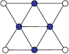
ii $F_{5}=\widehat{RL_{4}}$

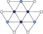
iii $F_{6}=\widehat{\widehat{K_{3}}}$

Figure 5: Chordal outerplanar graphs of degree $\Delta=4,5,6$, with $\mbox{\rm ind}=\Delta+1$.

Recall that when discussing the clique number or the chromatic number, we can by Lemma 2.2 assume $G$ to be biconnected. One of the main results of this section is the following theorem.

Theorem 4.1

For a chordal outerplanar graph $G$,

$$\omega(G^{2})=\chi(G^{2})=\left\{\begin{array}[]{cl}\Delta+2&\mbox{ if $\Delta=4$ and $F_{4}\subseteq G$,}\\ \Delta+1&\mbox{ in all other cases.}\end{array}\right.$$

We also derive a similar characterization of their inductiveness.

First note that the case $\Delta=2$ is trivial, since there is only one biconnected chordal outerplanar graph, namely $G=K_{3}$.

The case $\Delta\leq 3$ is easy, since there are only three biconnected chordal outerplanar graphs with $\Delta\leq 3$: $RL_{2}=P_{2}$ the 2-path, $RL_{3}=C_{3}=K_{3}$ the 3-cycle, and $RL_{4}$ is the 4-cycle with one diagonal. From this we deduce the following tree-like structure of $G$ in this case.

Lemma 4.2

Let $G$ be a chordal outerplanar graph of maximum degree $\Delta\leq 3$. Then the blocks of $G$ are among $\{RL_{2},RL_{3},RL_{4}\}$, where any two blocks from $\{RL_{3},RL_{4}\}$ are separated by at least one $RL_{2}$ block.

Considering the leaf blocks of $G$, we obtain from the structure given in Lemma 4.2 the following.

Theorem 4.3

For a chordal outerplanar graph $G$ with $\Delta\in\{2,3\}$, we have

$$\omega(G^{2})=\chi(G^{2})=\mbox{\rm ind}(G^{2})+1=\Delta+1.$$

The case $\Delta=4$ is more interesting, since it is the first case involving a “forbidden subgraph” condition for both the clique and the chromatic number of $G^{2}$. By considering the removal of a degree-2 vertex from $G$, we obtain the following by induction on $n=|V(G)|$.

Lemma 4.4

A graph $G$ is a biconnected chordal outerplanar graph with $\Delta=4$ if, and only if, $G\in\{F_{4}\}\cup\{RL_{n}:n\geq 5\}$.

• Clearly each graph in $\{F_{4}\}\cup\{RL_{n}:n\geq 5\}$ is biconnected and outerplanar. Conversely, let $G$ be a biconnected outerplanar graph on $n\geq 5$ vertices with maximum degree four. By removing a vertex $u$ of degree 2 from $G$, we obtain a biconnected outerplanar graph $G-u$ with $\Delta(G-u)\in\{3,4\}$, and hence equal to $RL_{4}$ or, by induction, from the set $\{F_{4}\}\cup\{RL_{n}:n\geq 5\}$. Since $G$ is of maximum degree $\Delta=4$ it is impossible that $G-u=F_{4}$. For the same reason if $G-u=RL_{4}$, then $G=RL_{5}$. Also, $G-u=RL_{5}$ only when $G\in\{RL_{6},F_{4}\}$, and lastly if $G-u=RL_{n}$ for some $n\geq 6$, then $G=RL_{n+1}$ must hold, thereby proving the lemma.     $\sqcap$$\sqcup$

Note that for $G=F_{4}$ we have $G^{2}=K_{6}$. Hence, in this case $\omega(G^{2})=\chi(G^{2})=6=\Delta+2$, while $\mbox{\rm ind}(G^{2})=5$.

Observe that $\mbox{\rm ind}(RL_{n}^{2})=4$, for any $n\geq 5$, since removing the last vertex in the square graph leaves the graph $RL^{2}_{n-1}$. Thus, $\omega(RL_{n}^{2})=\chi(RL_{n}^{2})=5$. By Lemmas 2.2 and 4.4 we have the following.

Theorem 4.5

For a chordal outerplanar graph $G$ with $\Delta=4$, we have

$$\omega(G^{2})=\chi(G^{2})=\mbox{\rm ind}(G^{2})+1=\left\{\begin{array}[]{cl}6&\mbox{ if }F_{4}\subseteq G,\\ 5&\mbox{ otherwise.}\end{array}\right.$$

So far we have characterized chordal outerplanar graphs in terms of the clique number, chromatic number and inductiveness of their squares when $\Delta\in\{2,3,4\}$. Before we continue with the analysis of the chordal cases of $\Delta\in\{5,6\}$, we need the following definition and a lemma.

Definition 4.6

Let $G$ be a graph. Call a subgraph $H\subseteq G$ on $h$ vertices an $h$-separator, or just a separator if it induces a clique in $G^{2}$ whose removal breaks $G^{2}$ into disconnected components.

The following lemma shows that it suffices to bound the clique number and chromatic number for graphs without separators.

Lemma 4.7

Let $G$ be a graph and $H$ a separator of $G$ with $G=G^{\prime}\cup G^{\prime\prime}$ and $H=G^{\prime}\cap G^{\prime\prime}$. Then we have

$$\omega(G^{2}) = \max\{\omega({G^{\prime}}^{2}),\omega({G^{\prime\prime}}^{2})\},$$

$$\chi(G^{2}) = \max\{\chi({G^{\prime}}^{2}),\chi({G^{\prime\prime}}^{2})\}.$$

• Since $G^{2}={G^{\prime}}^{2}\cup{G^{\prime\prime}}^{2}$ and ${G^{\prime}}^{2}\cap{G^{\prime\prime}}^{2}=H^{2}$, which is a clique, we have the stated clique number for $G^{2}$. Further, any optimal coloring of either ${G^{\prime}}^{2}$ or ${G^{\prime\prime}}^{2}$ can be extended to an optimal coloring of $G^{2}$ by a suitable permutation of the colors. Hence we have the lemma.     $\sqcap$$\sqcup$

Recall that a tree is full if there are no vertices of degree 2.

Lemma 4.8

Let $G$ be a biconnected chordal outerplanar graph with a full weak dual $T^{*}(G)$.

1. If $\Delta=5$, then $G=F_{5}$.

2. If $\Delta=6$, then $G\in\{F_{6}\}\cup\{\widehat{RL_{n}}:n\geq 5\}$.

• Since $G$ is chordal it is uniquely determined by a plane embedding of its full weak dual $T^{*}(G)$. If $\Delta\in\{5,6\}$, then $T^{*}(G)$ contains a path of length $\Delta-2$ and since $T^{*}(G)$ is full each internal vertex of this path must have degree of three. Therefore $T^{*}(G)$ has at least $2(\Delta-2)$ vertices and so $G$ has $n\geq 2(\Delta-1)$ vertices. The unique full tree on $2(\Delta-2)$ vertices is the weak dual of $G=\widehat{RL_{\Delta-1}}$ on $2(\Delta-1)$ vertices and with maximum degree $\Delta$. Proceeding by induction, assume $G$ has $n\geq 2(\Delta-1)$ vertices has a full weak dual $T^{*}(G)$ on $n-2\geq 2(\Delta-2)$ vertices. Removing two siblings from $T^{*}(G)$ whose parent is a leaf in the pruned tree $\mbox{\rm pr}(T^{*}(G))$ corresponds to removing two degree-2 vertices $u$ and $v$ from $G$ of distance 2 from each other in $G$, and obtaining $G^{\prime\prime}=G-\{u,v\}$. Now $\mbox{\rm pr}(T^{*}(G))=T^{*}(G^{\prime\prime})$ is full and has $n-4\geq 2(\Delta-3)\geq 4$ vertices, since its maximum degree is three.

  If $T^{*}(G^{\prime\prime})$ has four vertices, then it is the unique 4-star and $G^{\prime\prime}=F_{4}$. Hence $G=F_{5}$ and $\Delta=5$ here. Note that the number of vertices in any full tree with maximum degree of three is always even. Hence, there are no full trees on five or seven vertices.

  If $T^{*}(G^{\prime\prime})$ has six vertices, then $T^{*}(G^{\prime\prime})$ is unique and $G^{\prime\prime}=F_{5}$. Hence $G=\widehat{RL_{5}}$ in this case and $\Delta=6$.

  Otherwise $T^{*}(G^{\prime\prime})$ must have at least eight vertices and hence $G^{\prime\prime}$ has at least ten vertices. By induction hypothesis we have $G^{\prime\prime}\in\{F_{6}\}\cup\{\widehat{RL_{n}}:n\geq 5\}$. To have $G^{\prime\prime}=F_{6}$ is impossible, since that would create $G$ with $\Delta=8$. So $G^{\prime\prime}=\widehat{RL_{n}}$ for some $n\geq 5$. If $G^{\prime\prime}=\widehat{RL_{5}}$ then either $G=F_{6}$ or $G=\widehat{RL_{6}}$. Otherwise $G=\widehat{RL_{n-1}}$, which completes the proof.     $\sqcap$$\sqcup$

Theorem 4.9

Let $G$ be a biconnected chordal outerplanar graph with $\Delta\in\{5,6\}$. If $T^{*}(G)$ is not full, then either $G^{2}$ is a clique or $G$ has an $h$-separator where $h\in\{4,5,6,7\}$.

• Note that since $G$ is chordal, then every face corresponding to a vertex in $T^{*}(G)$ is bounded by a triangle. So for a given $T^{*}(G)$, the structure of $G$ is determined except for the degree-2 vertices of $G$. By assumption $T^{*}(G)$ has a degree-2 vertex. We consider the following three cases.

  If $T^{*}(G)$ has no vertex of degree 3, then $T^{*}(G)$ is a simple path. In this case it is easy to see that $G^{2}$ has a path decomposition consisting of cliques, where each clique is induced by a closed neighborhood of a vertex of $G$, necessarily of of size 5, 6 or 7. In particular, $G^{2}$ is by [6, Prop. 12.3.8] a chordal graph and is therefore a clique or has a 4-separator.

  Consider next the case where $T^{*}(G)$ has a degree-2 vertex $u^{*}$ that lies on a path connecting two degree-3 vertices of $T^{*}(G)$. If $e$ is the unique edge in $G$ bounding the triangular face $f$ corresponding to $u^{*}$ and the infinite face, then let $w\in V(G)$ be the vertex opposite the edge $e$ in the triangle $f$. Since $e$ and two other edges $e^{\prime}$ and $e^{\prime\prime}$ incident to $w$ in $G$ all bound the infinite face of $G$, we see that the closed neighborhood of $N_{G}[w]$ is an $h$-separator of $G$, where $h=d_{G}(w)+1\in\{5,6,7\}$.

  Lastly, consider the case where every degree-2 vertex of $T^{*}(G)$ lies on a path connecting a degree-3 vertex and a leaf of $T^{*}(G)$. In this case $T^{*}(G)$ must contain a degree-2 vertex $v^{*}$ that has a leaf $u^{*}$ as a neighbor. Let $u,v,w\in V(G)$ be the vertices bounding the triangular face $f$ corresponding to the leaf $u^{*}$, where $u$ has degree 2 in $G$ and $v$ has degree 2 in $G-u$. Note that $v^{*}$ is a leaf in $\mbox{\rm pr}(T^{*}(G))$. In this case $V=N_{G}[w]\setminus\{u\}$ induces a clique in $G^{2}$ which separates $u$ from the rest of the graph $G^{2}$. Since $T^{*}(G)$ has a vertex of degree 3, then $G^{2}-V$ has at least two components where one component consists of the singleton $u$. Hence, $V$ induces an $h$-separator of size $h=|V|=d_{G}(w)\in\{4,5,6\}$. This completes our proof.     $\sqcap$$\sqcup$

Note that $F_{5}^{2}$ is $K_{8}$ with two perpendicular diagonals removed when the vertices are located on a regular 8-gon. Therefore these two pairs of opposite nonadjacent vertices can be colored by the same color in $F_{5}^{2}$, and hence $\chi(F_{5}^{2})=\Delta+1=6$.

We note further that $F_{6}$ is biconnected chordal outerplanar graph with $\Delta=6$. Also, the subgraph $\widehat{K_{3}}$ in $F_{6}$ induces a clique in $F_{6}^{2}$, and hence each vertex there must have a unique color, say cyclically with colors $1,2,3,4,5,6$ starting with a degree-2 vertex of $\widehat{K_{3}}$. Of the remaining six vertices of $F_{6}$, color three of them with a new color 7, all of distance three apart, and the remaining three with the colors 1, 3 and 5. Hence $\chi(F_{6}^{2})=\Delta+1=7$.

To color ${\widehat{RL_{n}}}^{2}$ we can start by coloring the degree-2 vertices of $\widehat{RL_{n}}$ alternatively with colors 1 and 2 cyclically. The rest of the vertices, that constitute $RL_{n}$, we can then color with the remaining five available colors, since we have already that $\mbox{\rm ind}(RL_{n}^{2})=4$. Hence we have $\chi(RL_{n}^{2})=\Delta(RL_{n})+1=7$.

With the above in mind together with Lemmas 2.2, 4.7, and 4.8 and Theorems 3.1 and 4.9 we obtain in particular the following.

Corollary 4.10

For a chordal outerplanar graph $G$ with $\Delta\in\{5,6\}$ we have

$$\omega(G^{2})=\chi(G^{2})=\Delta+1.$$

Corollary 4.10 together with Theorems 4.3 and 4.5 complete the proof of Theorem 4.1 as well as the entries in Table LABEL:tab:Delta in the chordal case for $\Delta\in\{2,3,4,5,6\}$.

Observation 4.11

For each $\Delta\in\{4,5,6\}$, there are infinitely many biconnected chordal outerplanar graphs $G$ of maximum degree $\Delta$ with $\mbox{\rm ind}(G^{2})=\Delta+1$.

• It suffices to show that for each $\Delta\in\{4,5,6\}$ there are infinitely many biconnected outerplanar graphs $G$ whose squares are of minimum degree $\Delta+1$. Refer to Figure 5 for the appearance of the graphs.

  For $\Delta=4$, consider $F_{4}=\widehat{K_{3}}$, whose square is $K_{6}$ and hence has a minimum degree $\Delta+1$. By fusing together edges whose endvertices have degrees two and four, in two or more copies of $F_{4}$, we can construct an infinite family of such biconnected outerplanar graphs $G$ with $\Delta=4$ with $\mbox{\rm ind}(G^{2})=5$.

  For $\Delta=5$, consider $F_{5}$, whose square is $K_{8}$ with two perpendicular diagonals removed when the vertices are located on a regular 8-gon. Also in this case we can fuse together two edges with endvertices of degree 2 and 5, of two or more copies of $F_{5}$, and obtain an infinite family of such biconnected outerplanar graphs $G$ with $\Delta=5$ with $\mbox{\rm ind}(G^{2})=6$.

  Finally, for $\Delta=6$, consider $F_{6}$. In this case we have $\mbox{\rm ind}(F_{6}^{2})=7$, and also here we can fuse edges with endvertices of degree 2 and 4, of two or more copies of $F_{6}$, to form an infinite family of biconnected outerplanar graphs $G$ of maximum degree $\Delta=6$ and with $\mbox{\rm ind}(G^{2})=7$. This completes the proof.     $\sqcap$$\sqcup$

Remark: We note that $F_{4}^{2}=K_{6}$ is chordal, but neither $F_{5}^{2}$ nor $F_{6}^{2}$ are chordal, showing that the square of a chordal graph does not need to be chordal. This is consistent with the characterization of those chordal graphs whose squares are chordal given in [10].

Theorem 4.12

For a chordal outerplanar graph $G$, we have $\mbox{\rm ind}(G^{2})=\Delta$ or $\Delta+1$. Necessary and sufficient conditions that $\mbox{\rm ind}(G^{2})=\Delta+1$, are one of the following:

1. $\Delta=4$ and $F_{4}\subseteq G$,

2. $\Delta=5$ and $F_{5}\subseteq G$, or

3. $\Delta=6$ and one of $\{F_{6}\}\cup\{RL_{n}\}$, $n\geq 4$, is a subgraph of $G$.

5 Clique number

In this section we deal with the clique number of $G^{2}$. This parameter is the easiest to deal with. Nonetheless the exact computation of the clique number will rely on some results in previous Sections 3 and 4. Recall that by Lemma 2.2 we can assume $G$ to be biconnected. Further, $G$ is here not necessarily chordal.

Lemma 5.1

For an outerplanar graph $G$ we have $\omega(G^{2})\leq\Delta+2$, unless $G=C_{5}$. If $\Delta\geq 5$, then $\omega(G^{2})=\Delta+1$. For $\Delta\geq 6$ we further have that any clique with $\Delta+1$ vertices is the closed neighborhood of some vertex.

• Consider an induced subgraph $H_{k}$ of $G$ with $k+1$ vertices: a vertex $u$ and its neighbors $u_{1},u_{2},\ldots,u_{k}$ in a clockwise order in the plane embedding of $G$. Then only adjacent pairs $u_{i}$ and $u_{i+1}$, for $i=1,\ldots,k-1$, may be connected by an edge. Consider now a vertex $w$ that is not a neighbor of $u$. Then, $w$ can be adjacent to at most two neighbors of $u$ and only consecutive ones, by the outerplanarity property. If $k\geq 5$, then $w$ cannot be adjacent to both one of $u_{1}$ and $u_{2}$ and to one of $u_{k-1}$ and $u_{k}$. Thus, it must be of distance at least 3 from either $u_{1}$ or $u_{k}$. Hence, $H_{k}\cup\{w\}$ is not a clique in $G^{2}$. This shows that if a clique in $G^{2}$ contains a closed neighborhood of a vertex of degree $k\geq 5$, then the clique consists precisely of those $k+1$ vertices.

  Consider now the case $k=4$ and we have two vertices $w_{1}$ and $w_{2}$ that are non-neighbors of $u$. In order to be of distance at most 2 from both $u_{1}$ and $u_{4}$, a vertex must be adjacent to $u_{2}$ and $u_{3}$. But, in an outerplanar graph, not both $w_{1}$ and $w_{2}$ can be so. Hence, $H_{4}\cup\{w_{1},w_{2}\}$ does not form a clique. This shows that if a clique in $G^{2}$ contains a closed neighborhood of a vertex of degree $k=4$, then the clique consists of at most $k+2$ vertices, the vertices of the closed neighborhood plus a possibly additional vertex.

  Suppose now an induced subgraph $H$ of maximum degree 3 induces a 6-clique in $G$. Recall that by Lemma 2.2 we assume $H$ to be biconnected and therefore induced by a cycle. There can be at most two chords in $H$ and they must be disjoint since $\Delta(H)=3$. Then there are two vertices in $H$ of degree 2 that are of distance 3 in $H$. Further, since all vertices of $H$ lie on the outer face, there can be no vertex outside $H$ connecting them.

  From the above paragraphs we conclude that if a clique of $G^{2}$ contains $\Delta+1\geq 7$ vertices, it must be a closed neighborhood of a vertex of degree $\Delta$. Hence, the lemma.     $\sqcap$$\sqcup$

We conclude this section by quickly discussing matching lower bounds for $\omega(G^{2})$. Note, that we are here still under the assumption that $G$ is biconnected.

If $\Delta=2$, then $G=C_{k}$ is a cycle on $k\geq 3$ vertices and we clearly have

$$\omega(G^{2}) = \left\{\begin{array}[]{ll}\Delta+3&\mbox{ if }G=C_{5},\\ \Delta+2&\mbox{ if }G=C_{4},\\ \Delta+1&\mbox{ otherwise.}\\ \end{array}\right.$$

For $\Delta=3$ the upper bound of $\Delta+2$ is matched if $G$ is the graph obtained by adding one chord to the 5-cycle $C_{5}$.

For $\Delta\in\{4,5\}$ the matching upper bound of both $\Delta+2$ when $\Delta=4$ and $\Delta+1$ when $\Delta=5$ is obtain when $G=F_{4}$ shown in Figure 5.

If $\Delta\geq 6$, then by the above Lemma 5.1, the matching upper bound of $\Delta+1$ is obtained by a closed neighborhood of any vertex of degree $\Delta$.

Together with what was obtained in the previous Section 4, we therefore have all the entries for $\omega(G^{2})$ for an outerplanar graph $G$ (chordal or not) displayed in Table LABEL:tab:Delta.

6 The chromatic number

Recall that for an outerplanar graph $G$ with $\Delta\geq 7$ we have by Theorem 3.1 that $\mbox{\rm ind}(G^{2})\leq\Delta$ and hence $\chi(G^{2})\leq\Delta+1$ which is optimal. (In fact, Lemmas 2.2 and 3.8 also imply this.) Hence, we will assume throughout this section that $\Delta\leq 6$.

6.1 Cases with $\Delta\in\{2,3,5\}$

If $\Delta=2$, then we have an upper bound $\chi(G^{2})\leq\mbox{\rm ind}(G^{2})+1\leq\Delta+3$ and a matching lower bound is obtained when $G=C_{5}$. In fact, if $G$ is $P_{k}$ (resp. $C_{k}$) the path (resp. cycle) on $k$ vertices, then $\Delta=2$ and it can be verified that for $k\geq 2$ we have that

$$\chi(G^{2}) = \left\{\begin{array}[]{ll}3&\mbox{ if }G=P_{k}\cup C_{3k},\\ 4&\mbox{ if }G=(C_{3k+1}\cup C_{3k+2})\setminus C_{5},\\ 5&\mbox{ if }G=C_{5}.\end{array}\right.$$

Further, Greedy obtains an optimal coloring even when inductiveness is not a tight bound on the chromatic number, that is on $C_{n}$ for $n\geq 6$.

For $\Delta=3$ and $\Delta=5$, we have an upper bound of $\chi(G^{2})\leq\mbox{\rm ind}(G^{2})+1=\Delta+2$. If $G$ is the graph obtained by adding a chord to the 5-cycle $C_{5}$, then $G^{2}$ is a clique and hence the lower bound for $\chi(G^{2})=\Delta+2$ is obtained for $\Delta=3$.

Consider now the case $\Delta=5$. Let $G_{10}$ be the graph on ten vertices given in (i) in Figure ii.

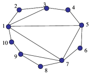
i $G_{10}$, $\chi(G^{2}_{10})=7=\Delta+2$

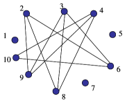
ii $\overline{G^{2}_{10}}$, the complement of the square of $G_{10}$

Figure 6: An example of a graph with $\Delta=5$ and $\chi=7=\Delta+2$

To see that $G_{10}^{2}$ requires $7$ colors, it is easiest to try to cover with cliques the complement graph $\overline{G_{10}^{2}}$, shown in (ii) in Figure ii. Each of the vertices $u_{1}$, $u_{5}$ and $u_{7}$ require their own clique, while for the remaining 7 vertices, there is no 3-clique. Hence, 7 cliques are required to cover $\overline{G_{10}^{2}}$. That is, 7 colors are required to color $G_{10}^{2}$. We note that $G_{10}$ has four edges with endvertices of degree 2 and 3 respectively. By fusing together two copies of $G_{10}$ along these edges in such a way that a degree-2 vertex in one copy is identified with a degree-3 vertex in another copy, we can make an infinite family of outerplanar graphs with $\Delta=5$, such that their square has chromatic number of $7$. We summarize in the following.

Theorem 6.1

There are infinitely many biconnected outerplanar graphs $G$ with maximum degree $\Delta=5$ such that $\chi(G^{2})=7$.

6.2 Cases with $\Delta=4$

Although it is impossible to obtain the tight bound of $\chi(G^{2})$ in the case when $\Delta=4$ via the inductiveness of $G^{2}$, our approach here will in similar fashion be inductive: We show how we can extend an optimal coloring of the square of a subgraph $G^{\prime}$ of $G$ to that of $G$.

Lemma 6.2

If $G$ is an outerplanar graph with maximum degree $\Delta=4$, then $\chi(G^{2})\leq 6$.

• By Lemma 2.2 we may assume $G$ to be biconnected. Since $\Delta=4$, then $\mbox{\rm pr}(T^{*}(G))$ is a proper tree and hence each 0-ss face $f$ has a parent $f^{\prime}$. If we can find a $k$-vertex in $G$, for $k\leq 5$, then a 6-coloring of $G$ follows by induction on $|V(G)|$. Observe that if $|f|\geq 4$, then each degree-2 vertex of $f$ is a 5-vertex. If $|f|=3$ and $|f^{\prime}|=3$, then the unique degree-2 vertex on $f$ is a 5-vertex. Additionally, if $|f|=3$ and $f^{\prime}$ has a face bounding the infinite face, then one 0-ss child of $f^{\prime}$ has a 5-vertex. Hence, we can assume that each 0-ss face is a 3-face whose parent $f^{\prime}$ satisfies $|f^{\prime}|\geq 4$ and has no edge bounding the infinite face.

  This implies one of the following two possibilities: (i) $f^{\prime}$ has a grandparent $f^{\prime\prime}$, or (ii) every edge of $f^{\prime}$ also bounds a child of $f^{\prime}$. In this case we can simply choose one designated child to play the role of the grandparent $f^{\prime\prime}$.

  Let $v_{1},\ldots,v_{k}$ be the vertices of $f^{\prime}$ where $k\geq 4$, and $v_{1}v_{k}$ be the edge bordering $f^{\prime\prime}$. Let $u_{1},\ldots,u_{k-1}$ be the vertices such that $v_{i}u_{i}v_{i+1}$ is a 0-ss child of $f^{\prime}$, for $i=1,\ldots,k-1$. Finally, since $\Delta=4$, $v_{1}$ and $v_{k}$ have at most one additional neighbor each; denote them by $x$ and $y$, respectively, which are not necessarily distinct.

  Let $G^{\prime}$ be the graph obtained after eliminating the face $f^{\prime}$ and its children (i.e., removing vertices $v_{2},\ldots,v_{k-1}$, $u_{1},\ldots,u_{k-1}$ and incident edges from $G$.) We show that a 6-coloring of ${G^{\prime}}^{2}$ can be extended to a 6-coloring of $G^{2}$. Since, this is the lone remaining case for $\Delta=4$, this yields the lemma.

  First case $k\in\{4,5\}$: For $k=4$ we first color $u_{1}$ and $u_{3}$ with a same color that is unused at $v_{1},v_{4},x,y$. Then color the vertices $v_{2},v_{3},u_{2}$ in a greedy fashion in this order, using at most 6 colors.

  For $k=5$ we first color $u_{1}$ and $v_{4}$ with a same color that is unused at $v_{1},v_{5},x,y$. Then color $v_{2}$ and $u_{4}$ with a same color that is unused at $v_{1},v_{5},x,y,u_{1}$ and $v_{4}$ (at most five colors used on these six vertices). Finally color $v_{3},u_{2},u_{3}$ in a greedy fashion in this order, using at most 6 colors.

  Second case $k\geq 6$: Note that in a coloring of $G^{2}$ in the previous case, $v_{1},u_{1},v_{2},u_{2},v_{3}$ all receive distinct colors since they induce a clique in $G^{2}$. Assume these colors are $1,2,3,4,5$ in this order respectively. Such a coloring can now be extended to a case of $k\geq 6$ by coloring $v_{1},u_{1},v_{2},u_{2},v_{3},u_{3},v_{4},u_{4},v_{5},u_{5},v_{6}$ using the colors $1,\ldots,6,1,\ldots 5$ in this order respectively. Since each case of $k\geq 6$ can be obtained by repeated use of such an extension, we have the lemma.     $\sqcap$$\sqcup$

6.3 Cases with $\Delta=6$

We now delve into the case where $G$ is an outerplanar graph with $\Delta=6$, and we will show that $\chi(G^{2})=\Delta+1=7$ always holds here. By Lemma 2.2 we shall assume $G$ to be biconnected and hence, by Lemma 2.4, its weak dual $T^{*}(G)$ to be a connected tree. As in Section 3, we will reduce our considerations to some key cases regarding the weak dual $T^{*}(G)$ of $G$. We will assume, unless otherwise stated, that $G$ is a biconnected outerplanar plane graph with $\Delta=6$ with $T^{*}(G)$ as a connected tree.

Assuming $\chi(G^{2})>7$, and that $G$ is minimal with this property (that is, any other graph with $\Delta=6$ has its square $7$-colorable), we note that we can assume that we do not have configurations (A) and (B) shown in Figure 2 nor configuration (C) in Figure 3, (since in those cases we would have a $6$-vertex, contradicting our assumption on $G$.). In other words, we may assume that (i) each face $f$ with $f^{*}$ a leaf in $T^{*}(G)$ is bounded by three or four edges, (ii) each 1-ss face $f$ is bounded by exactly three vertices, and (iii) each 1-ss face $f$ has at most on sibling in $T^{*}(G)$. We say that $G$ is 3-restricted if it satisfies all these assumptions (i), (ii) and (iii). In addition we have the following for the parent $f^{\prime}$ of $f$ in $T^{*}(G)$.

Lemma 6.3

If $G$ is 3-restricted, $f$ a 1-ss face and $|f^{\prime}|\geq 5$, then either $f$ or $f^{\prime}$ contains a $6$-vertex.

• Note that $f^{\prime}$ (that is to say ${f^{\prime}}^{*}$) is a leaf in the pruned tree $\mbox{\rm pr}(T^{*}(G))$. Let $f^{\prime}$ be bounded by the vertices $v_{0},\ldots,v_{\alpha}$ with $\alpha\geq 4$ and where $v_{0}v_{\alpha}$ it the edge in $G$ that boarders the grandparent $f^{\prime\prime}$ (that is to say, is dual to the edge in $T^{*}(G)$ incident to $f^{\prime}$). If $v_{i}$ and $v_{i+1}$ are on the boundary of either $f$ or its unique sibling $g$ (in the case that $f$ has a sibling $g$) for some $i\in\{1,\ldots,\alpha-2\}$, then the degree-two vertex on either $f$ or $g$ has degree at most five in $G^{2}$. Otherwise, all the $\alpha-2\geq 2$ edges $v_{1}v_{2},\ldots,v_{\alpha-2}v_{\alpha-1}$ bound the infinite face of $G$, in which case the $\alpha-3\geq 1$ vertices, $v_{2},\ldots,v_{\alpha-2}$, all are degree-two vertices with at most six neighbors in $G^{2}$. This completes the proof.     $\sqcap$$\sqcup$

Consider further the case for a 3-restricted $G$ where $f$ is a 1-ss face of $G$, the face $f^{\prime}$ is bounded by four vertices $v_{0},v_{1},v_{2},v_{3}$ and $f$ is bounded by $u,v_{1},v_{2}$ in such a way that the edges $v_{0}v_{1}$, $v_{1}v_{2}$ and $v_{2}v_{3}$ all bound the infinite face of $G-u$. In this case both $v_{1}$ and $v_{2}$ have degree three in $G$ and hence the degree-two vertex $u$ has four neighbors in $G^{2}$. To avoid any vertices of degree $\leq 6$ in $G^{2}$, we can therefore assume that if, for any 1-ss face $f$ with $f^{\prime}$ bounded by the four vertices $v_{0},v_{1},v_{2},v_{3}$, then the edge $v_{1}v_{2}$ must bound the infinite face of $G$.

To make further restrictions, assume that $G$ is a biconnected outerplanar graph that is induced by the cycle $C_{n}$ on the vertices $\{u_{1},\ldots,u_{n}\}$ in clockwise order. If $d_{G}(u_{3})=4$ and $u_{3}$ is adjacent to both $u_{1}$ and $u_{5}$ in $G$, then for any coloring of the square $G^{2}$ the vertices $u_{1},\ldots,u_{5}$ must all receive distinct colors, say $1,\ldots,5$ respectively, since $N_{G}[u_{3}]=\{u_{1},\ldots,u_{5}\}$ induces a clique in $G^{2}$. Consider the outerplanar graph $G^{\prime}$ obtained by first removing both the edges $u_{3}u_{4}$ and $u_{3}u_{5}$ and then connecting a new vertex $u_{3}^{\prime}$ to each of the vertices $u_{3},u_{4}$ and $u_{5}$. In this way $G$ becomes the contraction of $G^{\prime}$, namely $G={G^{\prime}}/u_{3}u_{3}^{\prime}$. Note that if $G$ has a maximum degree of $\Delta=6$, then so does $G^{\prime}$. In addition, given the mentioned coloring of $G^{2}$ where $u_{i}$ has color $i$ for $1\leq i\leq 5$, then we can obtain a coloring of ${G^{\prime}}^{2}$ by retaining the colors of $u_{i}$ from $G^{2}$ for all $i\not\in\{2,3,4\}$, and then assigning colors $3,2,4,3$ to the vertices $u_{2},u_{3},u_{3}^{\prime},u_{4}$ respectively.

Definition 6.4

A biconnected outerplanar graph $G$ with maximum degree $\Delta=6$ and a minimum number of vertices satisfying $\chi(G^{2})=8$ is called a minimal criminal.

Clearly each minimal criminal must be 3-restricted. What our discussion preceding the above definition means, in particular, is the following additional property of a potential minimal criminal $G$.

Theorem 6.5

If $G$ is a minimal criminal, then $G$ has no degree-two vertices with $\leq 6$ neighbors in $G^{2}$. Further, let $f$ be a 1-ss face of $G$.

1. If $f$ has no sibling, then $f^{\prime}$ is bounded by four vertices. Further, all the faces $f$, $f^{\prime}$ and $f^{\prime\prime}$ have exactly on vertex in common on their boundaries.

2. If $f$ has one sibling $g^{*}$, then $f^{\prime}$ is bounded by three vertices. Hence, all the faces $f$, $g$ and $f^{\prime}$ are bounded by exactly three vertices and edges.

• If $f$ has no sibling and $f^{\prime}$ is bounded by three vertices and edges, then the degree-two vertex $u$ bounding $f$ has $\leq 6$ neighbors in $G^{2}$. Then by minimality of $|V(G)|$, the square of $G-u$ can be colored by at most seven colors, and hence so can $G^{2}$, since there is at least on color left for $u$ among the seven colors available. If further $f^{\prime}$ is bounded by four vertices and the faces $f$, $f^{\prime}$ and $f^{\prime\prime}$ have no common vertex on their boundaries, then as previously noted, $u$ has exactly four neighbors in $G^{2}$ since both neighbors of $u$ have degree three in $G$.

  If $f$ has one sibling $g$, and $f^{\prime}$ is bounded by four vertices $v_{0},v_{1},v_{2},v_{3}$, then the edge $v_{1}v_{2}$ bounds neither $f$ nor $g$ (since otherwise either $f$ or $g$ has a degree-two vertex on its boundary with at most five neighbors in $G^{2}$) and therefore (assuming $f$ is to the left of $g$ in the plane embedding of $G$) we have that $v_{0}v_{1}$ bounds $f$, the edge $v_{2}v_{3}$ bounds $g$ and $v_{1}v_{2}$ bounds the infinite face of $G$. Again, by minimality of $n$ we have that the the square of the contracted graph $G/v_{1}v_{2}$ has a legitimate 7-coloring. By our above discussion preceding Definition 6.4, this coloring can then be extended to a 7-coloring of $G^{2}$, thereby contradicting the criminality of $G$. This complete the proof.     $\sqcap$$\sqcup$

What Theorem 6.5 implies, in particular, is that in a 3-restricted minimal criminal $G$, each configuration $C(f,f^{\prime})$ of $f$ and its parent $f^{\prime}$, where $f$ is 1-ss, is itself induced by a 5-cycle on the vertices $v_{1},v_{2},v_{3},v_{4},v_{5}$ in a clockwise order, and is of one of the following three types (note that if $f$ has a sibling $g$, then it is unique and we assume $g$ to be the right of $f$ in the planar embedding of $T^{*}(G)$ when viewed from $f^{\prime}$):

(a)

$C(f,f^{\prime})$ is the 5-cycle on $\{v_{1},v_{2},v_{3},v_{4},v_{5}\}$ in which $v_{3}$ is connected to $v_{1}$. Here $f$ is bounded by $\{v_{1},v_{2},v_{3}\}$ and $f^{\prime}$ is bounded by $\{v_{1},v_{3},v_{4},v_{5}\}$.

(b)

$C(f,f^{\prime})$ is the 5-cycle on $\{v_{1},v_{2},v_{3},v_{4},v_{5}\}$ in which $v_{3}$ is connected to $v_{5}$. Here $f$ is bounded by $\{v_{3},v_{4},v_{5}\}$ and $f^{\prime}$ is bounded by $\{v_{1},v_{2},v_{3},v_{5}\}$.

(c)

$C(f,f^{\prime})$ is the 5-cycle on $\{v_{1},v_{2},v_{3},v_{4},v_{5}\}$ in which $v_{3}$ is connected to both $v_{1}$ and $v_{5}$. Here $f$ is bounded by $\{v_{1},v_{2},v_{3}\}$, the face $g$ is bounded by $\{v_{3},v_{4},v_{5}\}$ and $f^{\prime}$ is bounded by $\{v_{1},v_{3},v_{5}\}$.

Here, for all the three types of configurations, it is assumed that the edge $v_{1}v_{5}$ bounds the face $f^{\prime\prime}$ as well as $f^{\prime}$.

Remarks: Note that as plane configurations (a) and (b) are mirror images of each other. Also, note that in all configurations, all the edges $v_{i}v_{i+1}$ where $1\leq i\leq 4$ of the 5-cycle that induces $C(f,f^{\prime})$, except one edge $v_{1}v_{5}$, bound the infinite face of $G$.

Convention: Let $G$ be a 3-restricted biconnected outerplanar graph with $\Delta=6$ such that for each 1-ss face $f$ of $G$ the configuration of $f$ and its parent $f^{\prime}$ is of type (a), (b) or (c) from above. Call such a $G$ fully restricted. Hence, a minimal criminal is always fully restricted.

Let $G$ be a biconnected outerplanar graph induced by the cycle $C_{n}$ on the vertices $\{u_{1},\ldots,u_{n}\}$ in clockwise order. Assume that $d_{G}(u_{4})=6$ and that $u_{4}$ is adjacent to $u_{1},u_{2},u_{3},u_{5},u_{6}$ and $u_{7}$. From $G$ we construct four other outerplanar graphs $\tilde{G}$, $G^{\prime}$, $G^{\prime\prime}$ and $G^{\prime\prime\prime}$ in the following way:

1. Let $\tilde{G}$ be obtained by replacing the edge $u_{1}u_{2}$ by the 2-path $(u_{1},x,u_{2})$.

2. Let $G^{\prime}$ be obtained from $G$ by replacing the edges $u_{1}u_{2}$ and $u_{6}u_{7}$ by the 2-paths $(u_{1},x,u_{2})$ and $(u_{6},y,u_{7})$ respectively.

3. Let $G^{\prime\prime}$ be obtained from $G$ by replacing the edge $u_{1}u_{2}$ by the 2-path $(u_{1},x,u_{2})$ and connecting the additional vertex $y$ to both $u_{6}$ and $u_{7}$.

4. Let $G^{\prime\prime\prime}$ be obtained from $G$ by connecting the additional vertex $x$ to both $u_{1}$ and $u_{2}$ and the additional vertex $y$ to $u_{6}$ and $u_{7}$.

Note that $G$ is a contraction of each of the graphs $\tilde{G}$, $G^{\prime}$, $G^{\prime\prime}$ and $G^{\prime\prime\prime}$, namely

$$\tilde{G}/u_{1}x=({G^{\prime}}/u_{1}x)/u_{6}y=({G^{\prime\prime}}/u_{1}x)/u_{6}y=({G^{\prime\prime\prime}}/u_{1}x)/u_{6}y=G.$$

Lemma 6.6

A 7-coloring of $G^{2}$ can be extended to a 7-coloring of ${\tilde{G}}^{2}$.

• Since $N_{G}[u_{4}]=\{u_{1},u_{2},u_{3},u_{4},u_{5},u_{6},u_{7}\}$ induces a clique in $G^{2}$, we may assume $u_{i}$ to have color $i$ for $1\leq i\leq 7$ in the 7-coloring of $G^{2}$. To obtain a 7-coloring of ${\tilde{G}}^{2}$ we retain the colors of $u_{i}$ from $G^{2}$ for all $i\not\in\{2,3,5\}$ and then assign colors $2,3,5,2$ to vertices $x,u_{2},u_{3},u_{5}$ respectively (note that we do not need to know the colors of all the neighbors of neither $u_{1}$ nor $u_{7}$ in the given 7-coloring of $G^{2}$).     $\sqcap$$\sqcup$

Convention: Let $G$ be a biconnected outerplanar graph $G$ with $\Delta=6$. Let $u$ be a degree-two vertex of $G$ that bounds a leaf-face $f$ of $T^{*}(G)$. If $(G-u)^{2}$ is provided with a 7-coloring, call $u$ c-simplicial if all the neighbors of $u$ in $G^{2}$ have collectively $\leq 6$ colors.

Note that $\tilde{G}$ from above cannot be a minimal criminal, since $u_{5}$ is c-simplicial; if we have a 7-coloring of $(\tilde{G}-u_{5})^{2}$ then we can extend it to a 7-coloring of ${\tilde{G}}^{2}$.

Our next theorem will provide our main tool for this section.

Theorem 6.7

If $G$ and the constructed graphs $G^{\prime}$, $G^{\prime\prime}$ and $G^{\prime\prime\prime}$ are as defined above, then none of the graphs $G^{\prime}$, $G^{\prime\prime}$ or $G^{\prime\prime\prime}$ are minimal criminals.

• If $G^{\prime}$ is a minimal criminal, then by definition $G^{2}$ has a legitimate 7-coloring. Again, we may assume $u_{i}$ to have color $i$ for $1\leq i\leq 7$. By retaining the colors of $u_{i}$ from $G^{2}$ for $i\not\in\{2,3,5,6\}$ and then assigning colors $2,3,6,2,5,6$ to the vertices $x,u_{2},u_{3},u_{5},u_{6},y$ respectively, we obtain a legitimate 7-coloring of ${G^{\prime}}^{2}$. Hence, $G^{\prime}$ cannot be a minimal criminal.

  If $G^{\prime\prime}$ is a minimal criminal, then $G^{2}$ has a legitimate 7-coloring. We can assume $u_{i}$ to have color $i$ for $1\leq i\leq 7$. By Lemma 6.6 we obtain a 7 coloring of ${\tilde{G}}^{2}$, as given in its proof. If $y$ is c-simplicial (w.r.t. this mentioned 7-coloring of $G^{2}$) then we can obtain a 7-coloring of ${G^{\prime\prime}}^{2}$. Therefore $y$ cannot be c-simplicial in this case. This means the neighbors of $u_{7}$ among $V(G)\setminus\{u_{2},\ldots,u_{6}\}$ have the colors $1,3$ and $5$ precisely, since $d_{G}(u_{7})=5$ and $d_{G^{\prime\prime}}(u_{7})=6$. In this case assign the colors $2,5,6,3,2,6$ to the vertices $x,u_{2},u_{3},u_{5},u_{6},y$. This is a legitimate 7-coloring of ${G^{\prime\prime}}^{2}$ and hence $G^{\prime\prime}$ cannot be a minimal criminal.

  If $G^{\prime\prime\prime}$ is a minimal criminal, then then $G^{2}=(G^{\prime\prime}-xy)^{2}$ has a legitimate 7-coloring. We can assume $u_{i}$ to have color $i$ for $1\leq i\leq 7$. If both $x$ and $y$ are c-simplicial, then we can extend the given coloring of $G^{2}$ to that of ${G^{\prime\prime\prime}}^{2}$, since $x$ and $y$ are of distance 3 or more from each other in $G^{\prime\prime\prime}$. If neither $x$ nor $y$ are c-simplicial, then we must have that the neighbors of $u_{1}$ among $V(G)\setminus\{u_{2},\ldots,u_{6}\}$ have the colors $5,6$ and $7$ precisely, and the neighbors of $u_{7}$ among $V(G)\setminus\{u_{2},\ldots,u_{6}\}$ have the colors $1,2$ and $3$ precisely. In this case we assign the colors colors $2,3,6,2,5,6$ to the vertices $x,u_{2},u_{3},u_{5},u_{6},y$ respectively (as in the case with $G^{\prime}$) and obtain a legitimate 7-coloring of ${G^{\prime\prime\prime}}^{2}$. We consider lastly the case where one of $x$ and $y$ is c-simplicial and the other is not. By symmetry, it suffices to consider the case where $x$ is c-simplicial and $y$ is not. The fact that $x$ is c-simplicial means that it can be assigned a color that must be from $\{5,6,7\}$ and thereby obtain a 7-coloring of $G^{\prime\prime\prime}-y$. Since $y$ is not c-simplicial means that the neighbors of $u_{7}$ among $V(G)\setminus\{u_{2},\ldots,u_{6}\}$ have the colors $1,2$ and $3$ precisely. We now consider the following three cases:

  $x$ has color $5$: In this case assign the colors $2,5,3,2,6,5$ to the vertices $x,u_{2},u_{3},u_{5},u_{6},y$, thereby obtaining a legitimate 7-coloring of ${G^{\prime\prime\prime}}^{2}$.

  $x$ has color $6$: In this case assign the colors $2,6,3,2,5,6$ to the vertices $x,u_{2},u_{3},u_{5},u_{6},y$, thereby obtaining a legitimate 7-coloring of ${G^{\prime\prime\prime}}^{2}$.

  $x$ has color $7$: Here $u_{1}$ and $u_{7}$ cannot be connected since both $x$ and $u_{7}$ have color $7$. In this case assign the colors $7,2,5,3,6,5$ to the vertices $x,u_{2},u_{3},u_{5},u_{6},y$, thereby obtaining a legitimate 7-coloring of ${G^{\prime\prime\prime}}^{2}$.

  This shows that $G^{\prime\prime\prime}$ cannot be a minimal criminal. This completes our proof.     $\sqcap$$\sqcup$

Remark: To test the legitimacy of the extended colorings we note first of all that the vertices $u_{1}$, $u_{4}$ and $u_{7}$ always keep their color from the one provided by $G^{2}$. In addition, the colors of the neighbors of $u_{1}$ among $\{u_{1},\ldots,u_{7}\}$ are the same, unless $x$ is not c-simplicial, which gives concrete information about the colors of the other neighbors of $u_{1}$. Similarly the colors of the neighbors of $u_{7}$ among $\{u_{1},\ldots,u_{7}\}$ are the same, unless (as for $x$) $y$ is not c-simplicial, which again gives concrete information about the colors of the remaining neighbors of $u_{7}$.

We are now ready for the proof of the following main result of this section.

Theorem 6.8

There is no minimal criminal; every biconnected outerplanar graph $G$ with $\Delta=6$ has $\chi(G^{2})=\Delta+1=7$.

• We will show that a minimal criminal must have the form of one of the graphs $G^{\prime}$, $G^{\prime\prime}$ or $G^{\prime\prime\prime}$, thereby obtaining a contradiction by Theorem 6.7.

  Assume $G$ is a minimal criminal, which must therefore be fully restricted. Since $\Delta=6$, each 1-ss face $f$ of $G$ has a parent $f^{\prime}$ and a grandparent $f^{\prime\prime}$ in $T^{*}(G)$. Hence, $f^{\prime\prime}$ (that is ${f^{\prime\prime}}^{*}$) is a leaf in $\mbox{\rm pr}^{2}(T^{*}(G))$ (or a single vertex). Since $G$ is fully restricted, the configuration $C(f,f^{\prime})$ in $G$ is induced by a 5-cycle on vertices $\{v_{1},v_{2},v_{3},v_{4},v_{5}\}$ in clockwise order and is of type (a), (b) or (c) mentioned earlier. Assume $f^{\prime\prime}$ is bounded by $u_{1},\ldots,u_{m}$ where $m\geq 3$. If $f^{\prime\prime}$ (that is ${f^{\prime\prime}}^{*}$) is not a single vertex but a leaf in $\mbox{\rm pr}^{2}(T^{*}(G))$, then let the edge $u_{m}u_{1}$ of $G$ be the dual edge of the unique edge with ${f^{\prime\prime}}^{*}$ as and endvertex in $\mbox{\rm pr}^{2}(T^{*}(G))$. In any case (whether ${f^{\prime\prime}}^{*}$ is a leaf or a single vertex in $\mbox{\rm pr}^{2}(T^{*}(G))$) at least one of the edges $u_{1}u_{2},\ldots,u_{m-1}u_{m}$ must be identified with an edge $v_{1}v_{5}$ of a configuration $C(f,f^{\prime})$ of type (a), (b) or (c).

  If there is an edge $u_{i}u_{i+1}$ bounding $f^{\prime\prime}$ and a configuration $C(f,f^{\prime})$ in such a way that the edge $v_{1}v_{5}$ is identified with $u_{i}u_{i+1}$ (i.e. $v_{1}=u_{i}$ and $v_{5}=u_{i+1}$) and such that either $d_{G}(v_{1})\leq 5$ or $d_{G}(v_{5})\leq 5$, then either the degree-two vertices $v_{1}$ or $v_{5}$ has $\leq 6$ neighbors in $G^{2}$ respectively. this means that a 7-coloring of either $G/v_{1}v_{2}$ or $G/v_{4}v_{5}$ can be used to extend to a 7-coloring of $G$. Therefore $G$ cannot be a minimal criminal in this case.

  We note that in order for $d_{G}(v_{1})=d_{G}(v_{5})=6$ for all configurations $C(f,f^{\prime})$, then every edge $u_{i}u_{i+1}$ for $1\leq i\leq m$ must be identified with an edge $v_{1}v_{5}$ of a configuration $C(f,f^{\prime})$. That is to say, none of the edges $u_{i}u_{i+1}$ can bound the infinite face of $G$. Since $m\geq 3$ we must, in particular, have that the edges $u_{1}u_{2}$ and $u_{2}u_{3}$ must be identified with edges $v_{1}v_{5}$ of configurations $C(f,f^{\prime})$ each of type (a), (b) or (c). If $d_{G}(u_{2})\leq 5$, then (as mentioned in previous paragraph) both configurations, to the left and right of $u_{2}$ in the plane embedding of $G$, contain a degree-two vertex with $\leq 6$ neighbors in $G^{2}$. In order for $d_{G}(u_{2})=6$ then the $C(f,f^{\prime})$ configuration to the left of $u_{2}$ in $G$, must be of type (b) or (c) and the configuration $C(f,f^{\prime})$ to the right of $u_{2}$ must be of type (a) or (c). We now finally discuss these cases separately. Here “Case (x,y)” will mean that configuration $C(f,f^{\prime})$ of type (x) is to the left of $u_{2}$ and configuration $C(f,f^{\prime})$ of type (y) is to the right of $u_{2}$.

  Case (b,a): Here $G$ is of type $G^{\prime}$ as stated in Theorem 6.7 (with $u_{2}$ in the role of $u_{4}$ mentioned there), and therefore cannot be a minimal criminal.

  Case (b,c): Here $G$ is of type $G^{\prime\prime}$ as stated in Theorem 6.7, and therefore cannot be a minimal criminal.

  Case (c,a): Here $G$ is a mirror image of a type $G^{\prime\prime}$ (previous case) as stated in Theorem 6.7, and therefore cannot be a minimal criminal.

  Case (c,c): Here $G$ is of type $G^{\prime\prime\prime}$ as stated in Theorem 6.7, and therefore cannot be a minimal criminal.

  This concludes the proof, that there is no minimal criminal, and hence the square of each biconnected outerplanar graph with $\Delta=6$ is 7-colorable.     $\sqcap$$\sqcup$

By Theorem 6.8 and Lemma 2.2 we have the following corollary.

Corollary 6.9

For every outerplanar graph $G$ with $\Delta=6$ we have $\chi(G^{2})=7$.

6.4 Greedy is not exact

We have observed that Greedy yields an optimal for coloring squares of outerplanar graphs whenever $\Delta\geq 7$ or $\Delta=2$. On many of the examples that we have constructed it also gives optimal colorings. It is therefore a natural question to ask whether it always obtains an optimal coloring. If not, one may ask for the case of chordal graphs, where we have seen that Greedy is also optimal for $\Delta=3$ and $\Delta=4$. Further evidence may be gathered by observing that it yields optimal colorings of $F_{4}$, $F_{5}$ and $RL_{n}$, since their squares are chordal.

We answer these questions in the negative by showing that the chordal graph $F_{6}$ is a counterexample.

Theorem 6.10

Greedy does not always output an optimal coloring of $F^{2}_{6}$.

• Suppose that the vertices of (iii) in Figure 5 are ordered so that first come the white vertices in the order shown on the figure (either from left-to-right or in a circular order). Then, Greedy will first color the white vertices with the first two colors. Now, the remaining six vertices must receive different colors, and none of them can use the first two colors, resulting in an 8-coloring.     $\sqcap$$\sqcup$

Acknowledgments

The authors are grateful to Steve Hedetniemi for his interest in this problem and for suggesting the writing of this article.

References

- [1] G. Agnarsson, M. M. Halldórsson. Coloring Powers of Planar Graphs. SIAM Journal of Discrete Mathematics, 16, No. 4, 651 – 662, (2003).
- [2] G. Agnarsson, M. M. Halldórsson. On Colorings of Squares of Outerplanar Graphs. Proceedings of the Fifteenth Annual ACM-SIAM Symposium On Discrete Algorithms (SODA 2004), New Orleans, 237 – 246, (2004).
- [3] K. Appel, W. Haken. Every Planar Graph is Four Colorable. Contemporary Mathematics 98, AMS, Providence, (1989).
- [4] O. Borodin, H. J. Broersmo, A. Glebov, and J. van den Heuvel. Stars and bunches in planar graphs. Part II: General planar graphs and colorings. CDAM Research Report Series 2002-05, (2002).
- [5] T. Calamoneri and R. Petreschi. -labeling subclasses of planar graphs. Journal of Parallel and Distributed Computing, 64(3):414–426, (2004).
- [6] R. Diestel. Graph Theory. Graduate Texts in Mathematics, GTM – 173, Springer Verlag, (1997).
- [7] M. M. Halldórsson and J. Radhakrishnan. Greed is good: Approximating independent sets in sparse and bounded-degree graphs. Algorithmica, 18: 145 – 163, (1997).
- [8] T. R. Jensen and B. Toft. Graph Coloring Problems. Wiley Interscience, (1995). http://www.imada.sdu.dk/Research/Graphcol/.
- [9] S. O. Krumke, M. V. Marathe, and S. S. Ravi. Approximation algorithms for channel assignment in radio networks. In Dial M for Mobility, 2nd International Workshop on Discrete Algorithms and Methods for Mobile Computing and Communications, Dallas, Texas, (1998).
- [10] R. Laskar and D. Shier. On Powers and Centers of Chordal Graphs. Discrete Applied Mathematics, 6: 139 – 147, (1983).
- [11] M. Molloy and M. R. Salavatipour. A bound on the chromatic number of the square of a planar graph. J. Combinatorial Theory (Series B), 94(2):189–213, (2005).
- [12] G. Wegner. Graphs with given diameter and a coloring problem. Technical report, University of Dortmund, (1977).
- [13] D. B. West. Introduction to Graph Theory. Prentice-Hall Inc., 2nd ed., (2001).
- [14] X. Zhou, Y. Kanari, and T. Nishizeki. Generalized vertex-colorings of partial -trees. IEICE Trans. Fundamentals, E83-A: 671 – 678, (2000).