Grassmann Integral Representation
for Spanning Hyperforests

Abstract

Given a hypergraph $G$, we introduce a Grassmann algebra over the vertex set, and show that a class of Grassmann integrals permits an expansion in terms of spanning hyperforests. Special cases provide the generating functions for rooted and unrooted spanning (hyper)forests and spanning (hyper)trees. All these results are generalizations of Kirchhoff’s matrix-tree theorem. Furthermore, we show that the class of integrals describing unrooted spanning (hyper)forests is induced by a theory with an underlying $\mathop{\rm OSP}\nolimits(1|2)$ supersymmetry.

PACS: 05.50.+q, 02.10.Ox, 11.10.Hi, 11.10.Kk

Keywords: Graph, hypergraph, forest, hyperforest, matrix-tree theorem, Grassmann algebra, Grassmann integral, $\sigma$-model, supersymmetry.

1 Introduction

Kirchhoff’s matrix-tree theorem [1, 2, 3] and its generalizations [4, 5, 6], which express the generating polynomials of spanning trees and rooted spanning forests in a graph as determinants associated to the graph’s Laplacian matrix, play a central role in electrical circuit theory [7, 8] and in certain exactly-soluble models in statistical mechanics [9, 10].

Like all determinants, those arising in Kirchhoff’s theorem can be rewritten as Gaussian integrals over fermionic (Grassmann) variables. Indeed, the use of Grassmann–Berezin calculus [11] has provided an interesting short-cut toward the classical matrix-tree result as well as generalizations thereof [6, 12]. For instance, Abdesselam [6] has obtained in a simple way the recent pfaffian-tree theorem [13, 14, 15] and has generalized it to a hyperpfaffian-cactus theorem.

In a recent letter [12] we proved a far-reaching generalization of Kirchhoff’s theorem, in which a large class of combinatorial objects are represented by suitable non-Gaussian Grassmann integrals. In particular, we showed how the generating function of spanning forests in a graph, which arises as the $q\to 0$ limit of the partition function of the $q$-state Potts model [16, 17, 18, 19], can be represented as a Grassmann integral involving a quadratic (Gaussian) term together with a special nearest-neighbor four-fermion interaction. Furthermore, this fermionic model possesses an $\mathop{\rm OSP}\nolimits(1|2)$ supersymmetry.

This fermionic formulation is also well-suited to the use of standard field-theoretic machinery. For example, in [12] we obtained the renormalization-group flow near the spanning-tree (free-field) fixed point for the spanning-forest model on the square lattice, and in [20] this was extended to the triangular lattice.

In the present paper we would like to extend the fermionic representation of spanning forests from graphs to hypergraphs. Hypergraphs are a generalization of graphs in which the edges (now called hyperedges) can connect more than two vertices [21, 22, 23]. In physics, hypergraphs arise quite naturally whenever one studies a $k$-body interaction with $k>2$. We shall show here how the generating function of spanning hyperforests in a hypergraph, which arises as the $q\to 0$ limit of the partition function of the $q$-state Potts model on the hypergraph [24], can be represented as a Grassmann integral involving a quadratic term together with special multi-fermion interactions associated to the hyperedges. Once again, this fermionic model possesses an $\mathop{\rm OSP}\nolimits(1|2)$ supersymmetry. This extension from graphs to hypergraphs is thus not only natural, but actually sheds light on the underlying supersymmetry.

Let us begin by recalling briefly the combinatorial identities proven in [12], which come in several levels of generality. Let $G=(V,E)$ be a finite undirected graph with vertex set $V$ and edge set $E$. To each edge $e$ we associate a weight $w_{e}$, which can be a real or complex number or, more generally, a formal algebraic variable; we then define the (weighted) Laplacian matrix $L=(L_{ij})_{i,j\in V}$ for the graph $G$ by

$$L_{ij}\;=\;\begin{cases}-w_{ij}&\hbox{if }i\neq j\\ \sum\limits_{k\neq i}w_{ik}&\hbox{if }i=j\end{cases}$$ (1.1)

We introduce, at each vertex $i\in V$, a pair of Grassmann variables $\psi_{i}$, ${\bar{\psi}}_{i}$, which obey the usual rules for Grassmann integration [11, 28]. Our identities show that certain Grassmann integrals over $\psi$ and ${\bar{\psi}}$ can be interpreted as generating functions for certain classes of combinatorial objects on $G$.

Our most general identity concerns the operators $Q_{\Gamma}$ associated to arbitrary connected subgraphs $\Gamma=(V_{\Gamma},E_{\Gamma})$ of $G$ via the formula

$$Q_{\Gamma}\;=\;\left(\prod_{e\in E_{\Gamma}}w_{e}\right)\left(\prod_{i\in V_{\Gamma}}{\bar{\psi}}_{i}\psi_{i}\right)\;.$$ (1.2)

(Note that each $Q_{\Gamma}$ is even and hence commutes with the entire Grassmann algebra.) We prove the very general identity

$$\int\!{\mathcal{D}}(\psi,{\bar{\psi}})\;\exp\!\left[{\bar{\psi}}L\psi+\sum\limits_{\Gamma}t_{\Gamma}Q_{\Gamma}\right]\;=\sum_{00112233\begin{array}[]{c}H\,\hbox{\scriptsize spanning}\subseteq G\\ H=(H_{1},\ldots,H_{\ell})\end{array}}\left(\prod_{e\in H}w_{e}\right)\prod_{\alpha=1}^{\ell}W(H_{\alpha})\;,$$ (1.3)

where the sum runs over spanning subgraphs $H\subseteq G$ consisting of connected components $(H_{1},\ldots,H_{\ell})$, and the weights $W(H_{\alpha})$ are defined by

$$W(H_{\alpha})\;=\;\sum_{\Gamma\prec H_{\alpha}}t_{\Gamma}\;,$$ (1.4)

where $\Gamma\prec H_{\alpha}$ means that $H_{\alpha}$ contains $\Gamma$ and contains no cycles other than those lying entirely within $\Gamma$.

Let us now specialize (1.3) to the case in which $t_{\Gamma}=t_{i}$ when $\Gamma$ consists of a single vertex $i$ with no edges, $t_{\Gamma}=u_{e}$ when $\Gamma$ consists of a pair of vertices $i,j$ linked by an edge $e$, and $t_{\Gamma}=0$ otherwise. We then have

$$\!\!\!\!\int\!{\mathcal{D}}(\psi,{\bar{\psi}})\,\exp\!\Big{[}{\bar{\psi}}L\psi\,+\,\sum\limits_{i}t_{i}{\bar{\psi}}_{i}\psi_{i}\,+\,\sum\limits_{\langle ij\rangle}u_{ij}w_{ij}{\bar{\psi}}_{i}\psi_{i}{\bar{\psi}}_{j}\psi_{j}\Big{]}$$

$$\qquad\qquad\;=\sum_{00112233\begin{array}[]{c}F\in{\cal F}(G)\\ F=(F_{1},\ldots,F_{\ell})\end{array}}\!\!\Biggl{(}\prod_{e\in F}w_{e}\Biggr{)}\prod_{\alpha=1}^{\ell}\Biggl{(}\sum_{i\in V(F_{\alpha})}t_{i}\,+\,\sum_{e\in E(F_{\alpha})}u_{e}\Biggr{)}\;,\qquad$$ (1.7)

where the sum runs over spanning forests $F$ in $G$ with components $F_{1},\ldots,F_{\ell}$; here $V(F_{\alpha})$ and $E(F_{\alpha})$ are, respectively, the vertex and edge sets of the tree $F_{\alpha}$.

If we further specialize (1.7) to $u_{e}=-\lambda$ for all edges $e$ (where $\lambda$ is a global parameter), we obtain

$$\!\!\!\!\int\!{\mathcal{D}}(\psi,{\bar{\psi}})\,\exp\!\Big{[}{\bar{\psi}}L\psi\,+\,\sum\limits_{i}t_{i}{\bar{\psi}}_{i}\psi_{i}\,-\,\lambda\sum\limits_{\langle ij\rangle}w_{ij}{\bar{\psi}}_{i}\psi_{i}{\bar{\psi}}_{j}\psi_{j}\Big{]}$$

$$\qquad\qquad\;=\sum_{00112233\begin{array}[]{c}F\in{\cal F}(G)\\ F=(F_{1},\ldots,F_{\ell})\end{array}}\!\!\Biggl{(}\prod_{e\in F}w_{e}\Biggr{)}\prod_{\alpha=1}^{\ell}\Biggl{(}\lambda\,+\,\sum_{i\in V(F_{\alpha})}(t_{i}-\lambda)\Biggr{)}\qquad$$ (1.10)

since $|E(F_{\alpha})|=|V(F_{\alpha})|-1$. If, in addition, we take $t_{i}=\lambda$ for all vertices $i$, then we obtain

$$&\!\!\!\!\int\!{\mathcal{D}}(\psi,{\bar{\psi}})\,\exp\!\Big{[}{\bar{\psi}}L\psi\,+\,\lambda\sum\limits_{i}{\bar{\psi}}_{i}\psi_{i}\,-\,\lambda\sum\limits_{\langle ij\rangle}w_{ij}{\bar{\psi}}_{i}\psi_{i}{\bar{\psi}}_{j}\psi_{j}\Big{]}\\ \qquad\qquad\;=\!\!\sum_{F\in{\cal F}(G)}\Biggl{(}\prod_{e\in F}w_{e}\Biggr{)}\;\lambda^{k(F)}\qquad\\ \qquad\qquad\;=\;\lambda^{|V|}\!\!\!\!\sum_{F\in{\cal F}(G)}\Biggl{(}\prod_{e\in F}\frac{w_{e}}{\lambda}\Biggr{)}$$ (1.11)

where $k(F)$ is the number of component trees in the forest $F$; this is the generating function of (unrooted) spanning forests of $G$. Furthermore, as discussed in [12] and in more detail in Section 7 below, the model (1.11) possesses an $\mathop{\rm OSP}\nolimits(1|2)$ invariance. If, by contrast, in (1.10) we take $\lambda=0$ but $\{t_{i}\}$ general, we obtain

$$\int\!{\mathcal{D}}(\psi,{\bar{\psi}})\,\exp\!\Big{[}{\bar{\psi}}L\psi\,+\,\sum\limits_{i}t_{i}{\bar{\psi}}_{i}\psi_{i}\,\Big{]}\;=\sum_{00112233\begin{array}[]{c}F\in{\cal F}(G)\\ F=(F_{1},\ldots,F_{\ell})\end{array}}\!\!\!\!\Biggl{(}\prod_{e\in F}w_{e}\Biggr{)}\prod_{\alpha=1}^{\ell}\Biggl{(}\sum_{i\in V(F_{\alpha})}t_{i}\Biggr{)}\;,$$ (1.12)

which is the formula representing rooted spanning forests (with a weight $t_{i}$ for each root $i$) as a fermionic Gaussian integral (i.e., a determinant) involving the Laplacian matrix (this formula is a variant of the so-called “principal-minors matrix-tree theorem”).

In this paper we shall not attempt to find the hypergraph analogue of the general formula (1.3), but shall limit ourselves to finding analogues of (1.7)–(1.12). The formulae to be presented here thus express the generating functions of unrooted or rooted spanning hyperforests in a hypergraph in terms of Grassmann integrals. In particular, the hypergraph generalization of (1.11) possesses the same $\mathop{\rm OSP}\nolimits(1|2)$ supersymmetry that (1.11) does (see Section 7).

The proof given here of all these identities is purely algebraic (and astonishingly simple); the crucial ingredient is to recognize the role and the rules of a certain Grassmann subalgebra (see Section 4). It turns out (Section 7) that this subalgebra is nothing other than the algebra of $\mathop{\rm OSP}\nolimits(1|2)$-invariant functions, though this is far from obvious at first sight. The unusual properties of this subalgebra (see Lemma 4.1) thus provide a deeper insight into the identities derived in [12] as well as their generalizations to hypergraphs, and indeed provide an alternate proof of (1.10)–(1.12). Pictorially, we can say that it is the underlying supersymmetry that is responsible for the cancellation of the cycles in the generating function, leaving only those spanning (hyper)graphs that have no cycles, namely, the (hyper)forests.

In particular, the limit of spanning hypertrees, which is easily extracted from the general expression for (rooted or unrooted) hyperforests, corresponds in the $\mathop{\rm OSP}\nolimits(1|2)$-invariant $\sigma$-model to the limit in which the radius of the supersphere tends to infinity, so that the nonlinearity due to the curvature of the supersphere disappears. However, the action is in general still non-quadratic, so that the model is not exactly soluble. (This is no accident: even the problem of determining whether there exists a spanning hypertree in a given hypergraph is NP-complete [29].) Only in the special case of ordinary graphs is the action purely quadratic, so that the partition function is given by a determinant, corresponding to the statement of Kirchhoff’s matrix-tree theorem.

The $\mathop{\rm OSP}\nolimits(1|2)$-invariant fermionic models discussed in [12] and the present paper can be written in three equivalent ways:

• As purely fermionic models, in which the supersymmetry is somewhat hidden.

• As $\sigma$-models with spins taking values in the unit supersphere in ${\mathbb{R}}^{1|2}$, in which the supersymmetry is manifest.

• As $N$-vector models [= $O(N)$-symmetric $\sigma$-models with spins taking values in the unit sphere of ${\mathbb{R}}^{N}$] analytically continued to $N=-1$.

The first two formulations (and their equivalence) are discussed in Section 7 of the present paper. Further aspects of this equivalence — notably, the role played by the Ising variables arising in (7.9) and neglected here — will be discussed in more detail elsewhere [30].

In a subsequent paper [31] we will discuss the Ward identities associated to the $\mathop{\rm OSP}\nolimits(1|2)$ supersymmetry, and their relation to the combinatorial identities describing the possible connection patterns among the (hyper)trees of a (hyper)forest.

The method proposed in the present paper has additional applications not considered here. With a small further effort, a class of Grassmann integrals wider than (5.2)/(6.3) — allowing products $\prod_{\alpha}f_{C_{\alpha}}^{(\lambda)}$ in the action in place of the single operators $f_{A}^{(\lambda)}$ — can be handled. Once again one obtains a graphical expansion in terms of spanning hyperforests, where now the weights have a more complicated dependence on the set of hyperedges, thus permitting a description of certain natural interaction patterns among the hyperedges of a hyperforest (see Remark at the end of Section 5). This extended model is, in fact, the most general Hamiltonian that is invariant under the $\mathop{\rm OSP}\nolimits(1|2)$ supersymmetry.

The plan of this paper is as follows: In Section 2 we recall the basic facts about graphs and hypergraphs that will be needed in the sequel. In Section 3 we define the $q$-state Potts model on a hypergraph and prove the corresponding Fortuin–Kasteleyn representation. (This section is unnecessary for the proof of the combinatorial identities that form the main focus of this paper, but it provides additional physical motivation.) In Section 4 we introduce the Grassmann algebra over the vertex set $V$, and study a subalgebra with interesting and unusual properties, which is generated by a particular family of even elements $f_{A}^{(\lambda)}$ with $A\subseteq V$. In Section 5 we study a very general partition function involving the operators $f_{A}^{(\lambda)}$, and we show how it can be expressed as a generating function of spanning hyperforests in a hypergraph with vertex set $V$. In Section 6 we study a somewhat more general Grassmann integral, which can be interpreted as a correlation function in this same Grassmann model; we show how it too can be expressed as a sum over spanning hyperforests. In Section 7 we show that in one special case — namely, the hypergraph generalization of (1.11) — the model studied in the preceding sections can be rewritten as an $\mathop{\rm OSP}\nolimits(1|2)$-invariant $\sigma$-model, and indeed is the most general $\mathop{\rm OSP}\nolimits(1|2)$-invariant Hamiltonian involving $\psi$ and ${\bar{\psi}}$. These $\sigma$-model formulae motivate the definition of $f_{A}^{(\lambda)}$ given in Section 4, which might otherwise remain totally mysterious.

In Appendix A we prove a determinantal formula for $f_{A}^{(\lambda)}$. In Appendix B we present a graphical formalism for proving both the classical matrix-tree theorem and numerous extensions thereof, which can serve as an alternative to the algebraic approach used in the main body of this paper.

Let us stress that everything in this paper is mathematically rigorous, with the possible exception of Section 7. Mathematicians unfamiliar with the Grassmann–Berezin calculus can find a brief introduction in [6, Section 2] or [32, Appendix A].

2 Graphs and hypergraphs

A (simple undirected finite) graph is a pair $G=(V,E)$, where $V$ is a finite set and $E$ is a collection (possibly empty) of 2-element subsets of $V$. The elements of $V$ are the vertices of the graph $G$, and the elements of $E$ are the edges. Usually, in a picture of a graph, vertices are drawn as dots and edges as lines (or arcs). Please note that, in the present definition, loops ( ) and multiple edges ( ) are not allowed. We write $|V|$ (resp. $|E|$) for the cardinality of the vertex (resp. edge) set; more generally, we write $|S|$ for the cardinality of any finite set $S$.

A graph $G^{\prime}=(V^{\prime},E^{\prime})$ is said to be a subgraph of $G$ (written $G^{\prime}\subseteq G$) in case $V^{\prime}\subseteq V$ and $E^{\prime}\subseteq E$. If $V^{\prime}=V$, the subgraph is said to be spanning. We can, by a slight abuse of language, identify a spanning subgraph $(V,E^{\prime})$ with its edge set $E^{\prime}$.

A walk (of length $k\geq 0$) connecting $v_{0}$ with $v_{k}$ in $G$ is a sequence $(v_{0},e_{1},v_{1},e_{2},v_{2},$ $\ldots,$ $e_{k},v_{k})$ such that all $v_{i}\in V$, all $e_{i}\in E$, and $v_{i-1},v_{i}\in e_{i}$ for $1\leq i\leq k$. A path in $G$ is a walk in which $v_{0},\ldots,v_{k}$ are distinct vertices of $G$ and $e_{1},\ldots,e_{k}$ are distinct edges of $G$. A cycle in $G$ is a walk in which

• $v_{0},\ldots,v_{k-1}$ are distinct vertices of $G$, and $v_{k}=v_{0}$

• $e_{1},\ldots,e_{k}$ are distinct edges of $G$; and

• $k\geq 2$.

The graph $G$ is said to be connected if every pair of vertices in $G$ can be connected by a walk. The connected components of $G$ are the maximal connected subgraphs of $G$. It is not hard to see that the property of being connected by a walk is an equivalence relation on $V$, and that the equivalence classes for this relation are nothing other than the vertex sets of the connected components of $G$. Furthermore, the connected components of $G$ are the induced subgraphs of $G$ on these vertex sets. We denote by $k(G)$ the number of connected components of $G$. Thus, $k(G)=1$ if and only if $G$ is connected.

A forest is a graph that contains no cycles. A tree is a connected forest. (Thus, the connected components of a forest are trees.) It is easy to prove, by induction on the number of edges, that

$$|E|\,-\,|V|\,+\,k(G)\;\geq\;0$$ (2.1)

for all graphs, with equality if and only if $G$ is a forest.

In a graph $G$, a spanning forest (resp. spanning tree) is simply a spanning subgraph that is a forest (resp. a tree). We denote by ${\mathcal{F}}(G)$ [resp. ${\mathcal{T}}(G)$] the set of spanning forests (resp. spanning trees) in $G$. As mentioned earlier, we will frequently identify a spanning forest or tree with its edge set.

Finally, we call a graph unicyclic if it contains precisely one cycle (modulo cyclic permutations and inversions of the sequence $v_{0},e_{1},v_{1},e_{2},v_{2},\ldots,e_{k},v_{k}$). It is easily seen that a connected unicyclic graph consists of a single cycle together with trees (possibly reduced to a single vertex) rooted at the vertices of the cycle.

Hypergraphs are the generalization of graphs in which edges are allowed to contain more than two vertices. Unfortunately, the terminology for hypergraphs varies substantially from author to author, so it is important to be precise about our own usage. For us, a hypergraph is a pair $G=(V,E)$, where $V$ is a finite set and $E$ is a collection (possibly empty) of subsets of $V$, each of cardinality $\geq 2$. The elements of $V$ are the vertices of the hypergraph $G$, and the elements of $E$ are the hyperedges (the prefix “hyper” can be omitted for brevity). Note that we forbid hyperedges of 0 or 1 vertices (some other authors allow these). We shall say that $A\in E$ is a $k$-hyperedge if $A$ is a $k$-element subset of $V$. A hypergraph is called $k$-uniform if all its hyperedges are $k$-hyperedges. Thus, a graph is nothing other than a 2-uniform hypergraph.

The definitions of subgraphs, walks, cycles, connected components, trees, forests and unicyclics given above for graphs were explicitly chosen in order to immediately generalize to hypergraphs: it suffices to copy the definitions verbatim, inserting the prefix “hyper” as necessary. See Figure 1 for examples of a forest and a hyperforest.

Figure 1: A forest (left) and a hyperforest (right), each with four components. Hyperedges with more than two vertices are represented pictorially as star-like polygons.

The analogue of the inequality (2.1) is the following:

Proposition 2.1

Let $G=(V,E)$ be a hypergraph. Then

$$\sum_{A\in E}(|A|-1)\,-\,|V|\,+\,k(G)\;\geq\;0\,,$$ (2.2)

with equality if and only if $G$ is a hyperforest.

Proofs can be found, for instance, in [22, p. 392, Proposition 4] or [34, pp. 278–279, Lemma].

Please note one important difference between graphs and hypergraphs: every connected graph has a spanning tree, but not every connected hypergraph has a spanning hypertree. Indeed, it follows from Proposition 2.1 that if $G$ is a $k$-uniform connected hypergraph with $n$ vertices, then $G$ can have a spanning hypertree only if $k-1$ divides $n-1$. Of course, this is merely a necessary condition, not a sufficient one! In fact, the problem of determining whether there exists a spanning hypertree in a given connected hypergraph is NP-complete (hence computationally difficult), even when restricted to the following two classes of hypergraphs:

• hypergraphs that are linear (each pair of edges intersect in at most one vertex) and regular of degree 3 (each vertex belongs to exactly three hyperedges); or

• 4-uniform hypergraphs containing a vertex which belongs to all hyperedges, and in which all other vertices have degree at most 3 (i.e., belong to at most three hyperedges)

(see [29, Theorems 3 and 4]). It seems to be an open question whether the problem remains NP-complete for 3-uniform hypergraphs.

Finally, let us discuss how a connected hypergraph can be built up one edge at a time. Observe first that if $G=(V,E)$ is a hypergraph without isolated vertices, then every vertex belongs to at least one edge (that is what “without isolated vertices” means!), so that $V=\bigcup\limits_{A\in E}A$. In particular this holds if $G$ is a connected hypergraph with at least two vertices. So let $G=(V,E)$ be a connected hypergraph with $|V|\geq 2$; let us then say that an ordering $(A_{1},\ldots,A_{m})$ of the hyperedge set $E$ is a construction sequence in case all of the hypergraphs $G_{\ell}=\big{(}\bigcup\limits_{i=1}^{\ell}A_{i},\,\{A_{1},\ldots,A_{\ell}\}\big{)}$ are connected ($1\leq\ell\leq m$). An equivalent condition is that $\Big{(}\bigcup\limits_{i=1}^{\ell-1}A_{i}\Big{)}\cap A_{\ell}\neq\varnothing$ for $2\leq\ell\leq m$. We then have the following easy result:

Proposition 2.2

Let $G=(V,E)$ be a connected hypergraph with at least two vertices. Then:

• There exists at least one construction sequence.

• If $G$ is a hypertree, then for any construction sequence $(A_{1},\ldots,A_{m})$ we have $\Big{|}\Big{(}\bigcup\limits_{i=1}^{\ell-1}A_{i}\Big{)}\cap A_{\ell}\Big{|}=1$ for all $\ell$ $(2\leq\ell\leq m)$.

• If $G$ is not a hypertree, then for any construction sequence $(A_{1},\ldots,A_{m})$ we have $\Big{|}\Big{(}\bigcup\limits_{i=1}^{\ell-1}A_{i}\Big{)}\cap A_{\ell}\Big{|}\geq 2$ for at least one $\ell$.

Proof. (a) The “greedy algorithm” works: Let $A_{1}$ be any hyperedge; and at each stage $\ell\geq 2$, let $A_{\ell}$ be any hyperedge satisfying $\Big{(}\bigcup\limits_{i=1}^{\ell-1}A_{i}\Big{)}\cap A_{\ell}\neq\varnothing$ (such a hyperedge has to exist, or else $G$ fails to be connected).

(b) and (c) are then easy consequences of Proposition 2.1.  $\Box$

3 Potts model on a hypergraph

Let $q$ be a positive integer, and let $S$ be a set of cardinality $q$. Then the $q$-state Potts model on the hypergraph $G=(V,E)$ is defined as follows [24]: At each vertex $i\in V$ we place a color (or spin) variable $\sigma_{i}\in S$. These variables interact via the Hamiltonian

$$\mathcal{H}_{\rm Potts}(\sigma)\;=\;-\sum_{A\in E}J_{A}\delta_{A}(\sigma)\;,$$ (3.1)

where $\{J_{A}\}_{A\in E}$ are a set of couplings associated to the hyperedges of $G$, and the Kronecker delta $\delta_{A}$ is defined for $A=\{i_{1},\ldots,i_{k}\}$ by

$$\delta_{A}(\sigma)\;=\;\begin{cases}1&\hbox{if }\sigma_{1}=\cdots=\sigma_{k}\\ 0&\hbox{otherwise }\end{cases}$$ (3.2)

The partition function $Z_{G}^{\rm Potts}$ is then the sum of $\exp[-\mathcal{H}_{\rm Potts}(\sigma)]$ over all configurations $\sigma=\{\sigma_{i}\}_{i\in V}$.

It is convenient to introduce the quantities $v_{A}=e^{J_{A}}-1$; we write ${\bf v}=\{v_{A}\}_{A\in E}$ for the collection of hyperedge weights. We can then prove the Fortuin–Kasteleyn (FK) representation [35, 36] for the hypergraph Potts model [24], by following exactly the same method as is used for graphs (see e.g. [19, Section 2.2]):

Proposition 3.1 (Fortuin–Kasteleyn representation)

Let $G=(V,E)$ be a hypergraph. Then, for integer $q\geq 1$, we have

$$Z_{G}^{\rm Potts}(q,{\bf v})\;\equiv\;\sum\limits_{\sigma\colon V\to S}\exp[-\mathcal{H}_{\rm Potts}(\sigma)]\;=\;\sum\limits_{E^{\prime}\subseteq E}q^{k(E^{\prime})}\prod\limits_{A\in E^{\prime}}v_{A}\;,$$ (3.3)

where $k(E^{\prime})$ denotes the number of connected components in the hypergraph $(V,E^{\prime})$.

Proof. We start by writing

$$Z_{G}^{\rm Potts}(q,{\bf v})\;=\;\sum\limits_{\sigma\colon V\to S}\exp[-\mathcal{H}_{\rm Potts}(\sigma)]\;=\;\sum\limits_{\sigma\colon V\to S}\prod\limits_{A\in E}\big{[}1+v_{A}\delta_{A}(\sigma)\big{]}\;.$$ (3.4)

Now expand out the product over $A\in E$, and let $E^{\prime}\subseteq E$ be the set of hyperedges for which the term $v_{A}\delta_{A}(\sigma)$ is taken. Now perform the sum over configurations $\{\sigma_{i}\}_{i\in V}$: in each connected component of the spanning subhypergraph $(V,E^{\prime})$ the color $\sigma_{i}$ must be constant, and there are no other constraints. Therefore,

$$Z_{G}^{\rm Potts}(q,{\bf v})\;=\;\sum\limits_{E^{\prime}\subseteq E}q^{k(E^{\prime})}\prod\limits_{A\in E^{\prime}}v_{A}\;,$$ (3.5)

as was to be proved.  $\Box$

Please note that the right-hand side of (3.3) is a polynomial in $q$; in particular, we can take it as the definition of the Potts-model partition function $Z_{G}(q,{\bf v})$ for noninteger $q$.

Let us discuss in particular the various types of $q\to 0$ limits that can be taken in the hypergraph Potts model, by following a straightforward generalization of the method that is used for graphs [19, Section 2.3]:

The simplest limit is to take $q\to 0$ with fixed ${\bf v}$. From the definition (3.3) we see that this selects out the spanning subhypergraphs $E^{\prime}\subseteq E$ having the smallest possible number of connected components; the minimum achievable value is of course $k(G)$ itself (= 1 in case $G$ is connected, as it usually is). We therefore have

$$\lim_{q\to 0}q^{-k(G)}Z_{G}(q,{\bf v})\;=\;C_{G}({\bf v})\;,$$ (3.6)

where

$$C_{G}({\bf v})\;=\;\!\!\!\sum\limits_{00112233\begin{array}[]{c}E^{\prime}\subseteq E\\ k(E^{\prime})=k(G)\end{array}}\!\!\prod_{A\in E^{\prime}}v_{A}$$ (3.7)

is the generating polynomial of “maximally connected spanning subhypergraphs” (= connected spanning subhypergraphs in case $G$ is connected).

A different limit can be obtained by taking $q\to 0$ with fixed values of $w_{A}=v_{A}/q^{|A|-1}$. From (3.3) we have

$$Z_{G}(q,\{q^{|A|-1}w_{A}\})\;=\;\sum\limits_{E^{\prime}\subseteq E}q^{k(E^{\prime})+\sum\limits_{A\in E^{\prime}}(|A|-1)}\prod\limits_{A\in E^{\prime}}w_{A}\;.$$ (3.8)

Using now Proposition 2.1, we see that the limit $q\to 0$ selects out the spanning hyperforests:

$$\lim_{q\to 0}q^{-|V|}Z_{G}(q,\{q^{|A|-1}w_{A}\})\;=\;F_{G}({\bf w})\;,$$ (3.9)

where

$$F_{G}({\bf w})\;=\;\sum\limits_{E^{\prime}\in{\mathcal{F}}(G)}\prod_{A\in E^{\prime}}w_{A}$$ (3.10)

is the generating polynomial of spanning hyperforests.

By a further limit we can obtain spanning hypertrees. To see this, assume first that $G$ is connected (otherwise there are no spanning hypertrees). In $C_{G}({\bf v})$, replace $v_{A}$ by $\lambda^{|A|-1}v_{A}$ and let $\lambda\to 0$; then we pick out the connected spanning subhypergraphs having the minimum value of $\sum_{A\in E^{\prime}}(|A|-1)$, which by Proposition 2.1 are precisely the spanning hypertrees:

$$\lim_{\lambda\to 0}\lambda^{-(|V|-1)}C_{G}(\{\lambda^{|A|-1}v_{A}\})\;=\;T_{G}({\bf v})\;,$$ (3.11)

where

$$T_{G}({\bf v})\;=\;\sum\limits_{E^{\prime}\in{\mathcal{T}}(G)}\prod_{A\in E^{\prime}}v_{A}$$ (3.12)

is the generating polynomial of spanning hypertrees. Alternatively, in $F_{G}({\bf w})$, replace $w_{A}$ by $\lambda^{|A|-1}w_{A}$ and let $\lambda\to\infty$; then we pick out the spanning hyperforests having the maximum value of $\sum_{A\in E^{\prime}}(|A|-1)$, which by Proposition 2.1 are those with the minimum number of connected components, i.e. again the spanning hypertrees:

$$\lim_{\lambda\to\infty}\lambda^{-(|V|-1)}F_{G}(\{\lambda^{|A|-1}w_{A}\})\;=\;T_{G}({\bf w})\;.$$ (3.13)

There is, however, one important difference between the graph case and the hypergraph case: as discussed in Section 2, every connected graph has a spanning tree, but not every connected hypergraph has a spanning hypertree. So the limits (3.11) and (3.13) can be zero.

4 A Grassmann subalgebra with unusual properties

Let $V$ be a finite set of cardinality $n$. For each $i\in V$ we introduce a pair $\psi_{i}$, ${\bar{\psi}}_{i}$ of generators of a Grassmann algebra (with coefficients in ${\mathbb{R}}$ or ${\mathbb{C}}$). We therefore have $2n$ generators, and the Grassmann algebra (considered as a vector space over ${\mathbb{R}}$ or ${\mathbb{C}}$) is of dimension $2^{2n}$.

For each subset $A\subseteq V$, we associate the monomial $\tau_{A}=\prod_{i\in A}{\bar{\psi}}_{i}\psi_{i}$, where $\tau_{\varnothing}=1$. Please note that all these monomials are even elements of the Grassmann algebra; in particular, they commute with the whole Grassmann algebra. Clearly, the elements $\{\tau_{A}\}_{A\subseteq V}$ span a vector space of dimension $2^{n}$. In fact, this vector space is a subalgebra, by virtue of the obvious relations

$$\tau_{A}\,\tau_{B}\;=\;\begin{cases}\tau_{A\cup B}&\hbox{if }A\cap B=\varnothing\\[5.69054pt] 0&\hbox{if }A\cap B\neq\varnothing\end{cases}$$ (4.1)

Let us now introduce another family of even elements of the Grassmann algebra, also indexed by subsets of $V$, which possesses very interesting and unusual properties. For each subset $A\subseteq V$ and each number $\lambda$ (in ${\mathbb{R}}$ or ${\mathbb{C}}$), we define the Grassmann element

$$f_{A}^{(\lambda)}\;=\;\lambda(1-|A|)\tau_{A}\,+\,\sum_{i\in A}\tau_{A\smallsetminus i}\,-\!\sum_{00112233\begin{array}[]{c}i,j\in A\\ i\neq j\end{array}}\!{\bar{\psi}}_{i}\psi_{j}\tau_{A\smallsetminus\{i,j\}}\,.$$ (4.2)

(The motivation for this curious formula will be explained in Section 7.) For instance, we have

$$f_{\varnothing}^{(\lambda)}&=\lambda\\ f_{\{i\}}^{(\lambda)}=1\qquad\hbox{for all }i\\ f_{\{i,j\}}^{(\lambda)}=-\lambda{\bar{\psi}}_{i}\psi_{i}{\bar{\psi}}_{j}\psi_{j}\,+\,{\bar{\psi}}_{i}\psi_{i}\,+\,{\bar{\psi}}_{j}\psi_{j}\,-\,{\bar{\psi}}_{i}\psi_{j}\,-\,{\bar{\psi}}_{j}\psi_{i}\\ =-\lambda{\bar{\psi}}_{i}\psi_{i}{\bar{\psi}}_{j}\psi_{j}\,+\,({\bar{\psi}}_{i}-{\bar{\psi}}_{j})(\psi_{i}-\psi_{j})$$ (4.3)

and in general

$$f_{\{i_{1},\ldots,i_{k}\}}^{(\lambda)}\;=\;\lambda(1-k)\tau_{\{i_{1},\ldots,i_{k}\}}\,+\,\sum_{\alpha=1}^{k}\tau_{\{i_{1},\ldots,\not{i_{\alpha}},\ldots,i_{k}\}}\,-\,\!\!\!\sum_{00112233\begin{array}[]{c}1\leq\alpha,\beta\leq k\\ \alpha\neq\beta\end{array}}\!\!\!{\bar{\psi}}_{i_{\alpha}}\psi_{i_{\beta}}\tau_{\{i_{1},\ldots,\not{i_{\alpha}},\ldots,\not{i_{\beta}},\ldots,i_{k}\}}\;.$$ (4.4)

(Whenever we write a set $\{i_{1},\ldots,i_{k}\}$, it is implicitly understood that the elements $i_{1},\ldots,i_{k}$ are all distinct.) Clearly, each $f_{A}^{(\lambda)}$ is an even element in the Grassmann algebra, and in particular it commutes with all the other elements of the Grassmann algebra.

The definition (4.2) can also be rewritten as

$$f_{A}^{(\lambda)}\;=\;\biggl{(}\lambda(1-|A|)+\sum\limits_{i,j\in A}\partial_{i}\bar{\partial}_{j}\biggr{)}\tau_{A}\;=\;\Bigl{(}\lambda(1-|A|)+\partial\bar{\partial}\Bigr{)}\tau_{A}$$ (4.5)

where $\partial_{i}=\partial/\partial\psi_{i}$ and $\bar{\partial}_{i}=\partial/\partial{\bar{\psi}}_{i}$ are the traditional anticommuting differential operators satisfying $\partial_{i}\psi_{j}=\delta_{ij}$, $\partial_{i}{\bar{\psi}}_{j}=0$, $\bar{\partial}_{i}{\bar{\psi}}_{j}=\delta_{ij}$, $\bar{\partial}_{i}\psi_{j}=0$ and the (anti-)Leibniz rule, while $\partial=\sum\limits_{i\in V}\partial_{i}$ and $\bar{\partial}=\sum\limits_{i\in V}\bar{\partial}_{i}$.

Let us observe that

$$f_{A}^{(\lambda)}\,\tau_{B}\;=\;\begin{cases}\tau_{A\cup B}&\hbox{if }|A\cap B|=1\\[5.69054pt] 0&\hbox{if }|A\cap B|\geq 2\end{cases}$$ (4.6)

as an immediate consequence of (4.1) [when $A\cap B=\{k\}$, only the second term in (4.2) with $i=k$ survives]. Note, finally, the obvious relations

$$\lim_{\lambda\to\infty}\frac{1}{\lambda}f_{A}^{(\lambda)}\;=\;(1-|A|)\tau_{A}$$ (4.7)

and

$$f_{A}^{(\lambda)}-f_{A}^{(\lambda^{\prime})}\;=\;(\lambda-\lambda^{\prime})(1-|A|)\tau_{A}\;.$$ (4.8)

We are interested in the subalgebra of the Grassmann algebra that is generated by the elements $f_{A}^{(\lambda)}$ as $A$ ranges over all nonempty subsets of $V$, for an arbitrary fixed value of $\lambda$. The key to understanding this subalgebra is the following amazing identity:

Lemma 4.1

Let $A,B\subseteq V$ with $A\cap B\neq\varnothing$. Then

$$f_{A}^{(\lambda)}\,f_{B}^{(\lambda)}\;=\;\begin{cases}f_{A\cup B}^{(\lambda)}&\textrm{if }|A\cap B|=1\\[5.69054pt] 0&\textrm{if }|A\cap B|\geq 2\end{cases}$$ (4.9)

More generally,

$$f_{A}^{(\lambda)}\,f_{B}^{(\lambda^{\prime})}\;=\;\begin{cases}f_{A\cup B}^{(\lambda^{\prime\prime})}&\textrm{if }|A\cap B|=1\\[5.69054pt] 0&\textrm{if }|A\cap B|\geq 2\end{cases}$$ (4.10)

where $\lambda^{\prime\prime}$ is the weighted average

$$\lambda^{\prime\prime}\;=\;\frac{(|A|-1)\lambda+(|B|-1)\lambda^{\prime}}{|A|+|B|-2}\;=\;\frac{(|A|-1)\lambda+(|B|-1)\lambda^{\prime}}{|A\cup B|-1}\;.$$ (4.11)

First proof. The formula (4.10) can be proven by a direct (but lengthy) calculation within the Grassmann algebra that makes explicit a sort of fermionic-bosonic cancellation. Details can be found in the first preprint version of this article (arXiv:0706.1509v1); see especially footnote 10 there.  $\Box$

Second proof. We are grateful to an anonymous referee for suggesting the following simple and elegant proof using the differential operators $\partial$ and $\bar{\partial}$:

Since $\partial^{2}=\bar{\partial}^{2}=0$, we have

$$\left(\partial\bar{\partial}\tau_{A}\right)\left(\partial\bar{\partial}\tau_{B}\right)\;=\;\partial\bar{\partial}\left(\tau_{A}\partial\bar{\partial}\tau_{B}\right)\;=\;\partial\bar{\partial}\left(\tau_{B}\partial\bar{\partial}\tau_{A}\right)\;,$$ (4.12)

so that

$$f_{A}^{(\lambda)}\,f_{B}^{(\lambda^{\prime})} = \lambda(1-|A|)\tau_{A}\partial\bar{\partial}\tau_{B}\,+\,\lambda^{\prime}(1-|B|)\tau_{B}\partial\bar{\partial}\tau_{A}$$ (4.13)

$$\quad+\,\lambda\lambda^{\prime}(1-|A|)(1-|B|)\tau_{A}\tau_{B}\,+\,\partial\bar{\partial}\left(\tau_{A}\partial\bar{\partial}\tau_{B}\right)\;.$$

If $|A\cap B|\geq 1$, then $\tau_{A}\tau_{B}=0$ and

$$\tau_{A}\partial\bar{\partial}\tau_{B}\;=\;\tau_{B}\partial\bar{\partial}\tau_{A}\;=\;\begin{cases}\tau_{A\cup B}&\textrm{if $|A\cap B|=1$}\\[5.69054pt] 0&\textrm{if $|A\cap B|\geq 2$}\end{cases}$$ (4.14)

This proves (4.10).  $\Box$

As a first consequence of Lemma 4.1, we have:

Corollary 4.2

Let $A\subseteq V$ with $|A|\geq 2$. Then the Grassmann element $f_{A}^{(\lambda)}$ is nilpotent of order 2, i.e.

$$\big{(}f_{A}^{(\lambda)}\big{)}^{2}=0\,.$$

In particular, a product $\prod_{i=1}^{m}f_{A_{i}}^{(\lambda)}$ vanishes whenever there are any repetitions among the $A_{1},\ldots,A_{m}$. So we can henceforth concern ourselves with the case in which there are no repetitions; then $E=\{A_{1},\ldots,A_{m}\}$ is a set (as opposed to a multiset) and $G=(V,E)$ is a hypergraph.

By iterating Lemma 4.1 and using Proposition 2.2, we easily obtain:

Corollary 4.3

Let $G=(V,E)$ be a connected hypergraph. Then

$$\prod_{A\in E}f_{A}^{(\lambda)}\;=\;\begin{cases}f_{V}^{(\lambda)}&\textrm{if $G$ is a hypertree}\\[5.69054pt] 0&\textrm{if $G$ is not a hypertree}\end{cases}$$ (4.15)

More generally,

$$\prod_{A\in E}f_{A}^{(\lambda_{A})}\;=\;\begin{cases}f_{V}^{(\lambda_{\star})}&\textrm{if $G$ is a hypertree}\\[5.69054pt] 0&\textrm{if $G$ is not a hypertree}\end{cases}$$ (4.16)

where $\lambda_{\star}$ is the weighted average

$$\lambda_{\star}\;=\;\frac{\,\sum\limits_{A\in E}(|A|-1)\lambda_{A}\,}{\sum\limits_{A\in E}(|A|-1)}\;=\;\frac{\,\sum\limits_{A\in E}(|A|-1)\lambda_{A}\,}{\rule{0.0pt}{11.5pt}\bigl{|}\bigcup\limits_{A\in E}A\bigr{|}-1}\;\,.$$ (4.17)

We are now ready to consider the subalgebra of the Grassmann algebra that is generated by the elements $f_{A}^{(\lambda)}$ as $A$ ranges over all nonempty subsets of $V$. Recall first that a partition of $V$ is a collection ${\mathcal{C}}=\{C_{\gamma}\}$ of disjoint nonempty subsets $C_{\gamma}\subseteq V$ that together cover $V$. We denote by $\Pi(V)$ the set of partitions of $V$. If $V$ has cardinality $n$, then $\Pi(V)$ has cardinality $B(n)$, the $n$-th Bell number [37, pp. 33–34]. We remark that $B(n)$ grows asymptotically roughly like $n!$ [38, Sections 6.1–6.3].

The following corollary specifies the most general product of factors $f_{A}^{(\lambda)}$. Of course, there is no need to consider sets $A$ of cardinality 1, since $f_{\{i\}}^{(\lambda)}=1$.

Corollary 4.4

Let $E$ be a collection (possibly empty) of subsets of $V$, each of cardinality $\geq 2$.

• If the hypergraph $G=(V,E)$ is a hyperforest, and $\{C_{\gamma}\}$ is the partition of $V$ induced by the decomposition of $G$ into connected components, then $\prod\limits_{A\in E}f_{A}^{(\lambda)}=\prod\limits_{\gamma}f_{C_{\gamma}}^{(\lambda)}$. More generally, $\prod\limits_{A\in E}f_{A}^{(\lambda_{A})}=\prod\limits_{\gamma}f_{C_{\gamma}}^{(\lambda_{\gamma})}$, where $\lambda_{\gamma}$ is the weighted average (4.17) taken over the hyperedges contained in $C_{\gamma}$.

• If the hypergraph $G=(V,E)$ is not a hyperforest, then $\prod\limits_{A\in E}f_{A}^{(\lambda)}=0$, and more generally $\prod\limits_{A\in E}f_{A}^{(\lambda_{A})}=0$.

Proof. It suffices to apply Corollary 4.3 separately in each set $C_{\gamma}$, where $\{C_{\gamma}\}$ is the partition of $V$ induced by the decomposition of $G$ into connected components.  $\Box$

It follows from Corollary 4.4 that any polynomial (or power series) in the $\{f_{A}^{(\lambda)}\}$ can be written as a linear combination of the quantities $f_{\mathcal{C}}^{(\lambda)}=\prod_{\gamma}f_{C_{\gamma}}^{(\lambda)}$ for partitions ${\mathcal{C}}=\{C_{\gamma}\}\in\Pi(V)$.

Using the foregoing results, we can simplify the Boltzmann weight associated to a Hamiltonian of the form

$$\mathcal{H}\;=\;-\sum_{A\in E}w_{A}f_{A}^{(\lambda)}\;.$$ (4.18)

Corollary 4.5

Let $G=(V,E)$ be a hypergraph (that is, $E$ is a collection of subsets of $V$, each of cardinality $\geq 2$). Then

$$\exp\Biggl{(}\sum_{A\in E}w_{A}f_{A}^{(\lambda)}\Biggr{)}\;=\!\!\sum_{00112233\begin{array}[]{c}F\in{\mathcal{F}}(G)\\ F=(F_{1},\ldots,F_{\ell})\end{array}}\!\!\Biggl{(}\prod\limits_{A\in F}w_{A}\Biggr{)}\,\prod_{\alpha=1}^{\ell}f_{V(F_{\alpha})}^{(\lambda)}\,,$$ (4.19)

where the sum runs over spanning hyperforests $F$ in $G$ with components $F_{1},\ldots,F_{\ell}$, and $V(F_{\alpha})$ is the vertex set of the hypertree $F_{\alpha}$. More generally,

$$\exp\Biggl{(}\sum_{A\in E}w_{A}f_{A}^{(\lambda_{A})}\Biggr{)}\;=\!\!\sum_{00112233\begin{array}[]{c}F\in{\mathcal{F}}(G)\\ F=(F_{1},\ldots,F_{\ell})\end{array}}\!\!\Biggl{(}\prod\limits_{A\in F}w_{A}\Biggr{)}\,\prod_{\alpha=1}^{\ell}f_{V(F_{\alpha})}^{(\lambda_{\alpha})}\,,$$ (4.20)

where $\lambda_{\alpha}$ is the weighted average (4.17) taken over the hyperedges contained in the hypertree $F_{\alpha}$.

Proof. Since the $f_{A}^{(\lambda_{A})}$ are nilpotent of order 2 and commuting, we have

$$\exp\Biggl{(}\sum_{A\in E}w_{A}f_{A}^{(\lambda_{A})}\Biggr{)}&=\prod\limits_{A\in E}\Big{(}1+w_{A}f_{A}^{(\lambda_{A})}\Big{)}\\ =\sum\limits_{E^{\prime}\subseteq E}\Biggl{(}\prod_{A\in E^{\prime}}w_{A}\Biggr{)}\Biggl{(}\prod_{A\in E^{\prime}}f_{A}^{(\lambda_{A})}\Biggr{)}\;.$$ (4.21)

Using now Corollary 4.4, we see that the contribution is nonzero only when $(V,E^{\prime})$ is a hyperforest, and we obtain (4.19)/(4.20).  $\Box$

In a separate paper [39] we shall study in more detail the Grassmann subalgebra that is generated by the elements $f_{A}^{(\lambda)}$ as $A$ ranges over all nonempty subsets of $V$. In the present section we have seen that any element of this subalgebra can be written as a linear combination of the quantities $f_{\mathcal{C}}^{(\lambda)}=\prod_{\gamma}f_{C_{\gamma}}^{(\lambda)}$ for partitions ${\mathcal{C}}=\{C_{\gamma}\}\in\Pi(V)$. It turns out that the quantities $f_{\mathcal{C}}^{(\lambda)}$ are linearly dependent (i.e., an overcomplete set) as soon as $|V|\geq 4$. We shall show [39], in fact, that a vector-space basis for the subalgebra in question is given by the quantities $f_{\mathcal{C}}^{(\lambda)}$ as ${\mathcal{C}}$ ranges over all non-crossing partitions of $V$ (relative to any fixed total ordering of $V$). It follows that the vector-space dimension of this subalgebra is given by the Catalan number $C_{n}=\frac{1}{n+1}\binom{2n}{n}$, where $n=|V|$. This is vastly smaller than the Bell number $B(n)$, which is the dimension that the subspace would have if the $f_{\mathcal{C}}^{(\lambda)}$ were linearly independent. [Indeed, one can see immediately that the $\{f_{\mathcal{C}}^{(\lambda)}\}$ must be linearly dependent for all sufficiently large $n$, simply because the entire Grassmann algebra has dimension only $4^{n}\ll B(n)$.] It also turns out [39] that all the relations among the $\{f_{\mathcal{C}}^{(\lambda)}\}$ are generated (as an ideal) by the elementary relations $R_{abcd}=0$, where

$$R_{abcd}\;=\;\lambda f_{\{a,b,c,d\}}^{(\lambda)}\,-\,f_{\{b,c,d\}}^{(\lambda)}\,-\,f_{\{a,c,d\}}^{(\lambda)}\,-\,f_{\{a,b,d\}}^{(\lambda)}\,-\,f_{\{a,b,c\}}^{(\lambda)}\\ \,+\,f_{\{a,b\}}^{(\lambda)}f_{\{c,d\}}^{(\lambda)}\,+\,f_{\{a,c\}}^{(\lambda)}f_{\{b,d\}}^{(\lambda)}\,+\,f_{\{a,d\}}^{(\lambda)}f_{\{b,c\}}^{(\lambda)}$$ (4.22)

and $a,b,c,d$ are distinct vertices.

5 Grassmann integrals for counting spanning hyperforests

For any subset $A\subseteq V$ and any vector ${\bf t}=(t_{i})_{i\in V}$ of vertex weights, let us define the integration measure

$$\mathcal{D}_{A,{\bf t}}(\psi,{\bar{\psi}})\;:=\;\prod_{i\in A}d{\psi_{i}}\,d{{\bar{\psi}}_{i}}\,e^{t_{i}{\bar{\psi}}_{i}\psi_{i}}\,.$$ (5.1)

Our principal goal in this section is to provide a combinatorial interpretation, in terms of spanning hyperforests, for the general Grassmann integral (“partition function”)

$$Z&=\int\mathcal{D}(\psi,{\bar{\psi}})\,\exp\biggl{[}\,\sum_{i}t_{i}{\bar{\psi}}_{i}\psi_{i}\,+\,\sum_{A\in E}w_{A}f_{A}^{(\lambda)}\biggr{]}\\ =\int\mathcal{D}_{V,{\bf t}}(\psi,{\bar{\psi}})\,\exp\biggl{[}\,\sum_{A\in E}w_{A}f_{A}^{(\lambda)}\biggr{]}\;,$$ (5.2)

where $G=(V,E)$ is an arbitrary hypergraph (that is, $E$ is an arbitrary collection of subsets of $V$, each of cardinality $\geq 2$) and the $\{w_{A}\}_{A\in E}$ are arbitrary hyperedge weights. We also handle the slight generalization in which a separate parameter $\lambda_{A}$ is used for each hyperedge $A$.

Our basic results are valid for an arbitrary vector ${\bf t}=(t_{i})_{i\in V}$ of “mass terms”. However, as we shall see, the formulae simplify notably if we specialize to the case in which $t_{i}=\lambda$ for all $i\in V$. This is not an accident, as it corresponds to the case in which the action is $\mathop{\rm OSP}\nolimits(1|2)$-invariant (see Section 7).

We begin with some formulae that allow us to integrate over the pairs of variables $\psi_{i},{\bar{\psi}}_{i}$ one at a time:

Lemma 5.1

Let $A\subseteq V$ and $i\in V$. Then:

• ${\displaystyle\int}d{\psi_{i}}\,d{{\bar{\psi}}_{i}}\,e^{t_{i}{\bar{\psi}}_{i}\psi_{i}}\,\tau_{A}\;=\;{\displaystyle\begin{cases}\tau_{A\smallsetminus i}&\textrm{if }i\in A\\[5.69054pt] t_{i}\tau_{A}&\textrm{if }i\notin A\end{cases}}$

• ${\displaystyle\int}d{\psi_{i}}\,d{{\bar{\psi}}_{i}}\,e^{t_{i}{\bar{\psi}}_{i}\psi_{i}}\,f_{A}^{(\lambda)}\;=\;{\displaystyle\begin{cases}f_{A\smallsetminus i}^{(\lambda)}\,+\,(t_{i}-\lambda)\tau_{A\smallsetminus i}&\textrm{if }i\in A\\[5.69054pt] t_{i}f_{A}^{(\lambda)}&\textrm{if }i\notin A\end{cases}}$

Proof. (a) is obvious, as is (b) when $i\notin A$. To prove (b) when $i\in A$, we write

$$f_{A}^{(\lambda)}\;=\;\lambda(1-|A|)\tau_{A}\,+\,\sum_{j\in A}\tau_{A\smallsetminus j}\,-\!\sum_{00112233\begin{array}[]{c}j,k\in A\\ j\neq k\end{array}}\!{\bar{\psi}}_{j}\psi_{k}\tau_{A\smallsetminus\{j,k\}}$$ (5.3)

and integrate with respect to $d{\psi_{i}}\,d{{\bar{\psi}}_{i}}\,e^{t_{i}{\bar{\psi}}_{i}\psi_{i}}$. We obtain

$$\lambda(1-|A|)\tau_{A\smallsetminus i}\,+\,t_{i}\tau_{A\smallsetminus i}\,+\,\sum_{j\in A\smallsetminus i}\tau_{A\smallsetminus\{i,j\}}\,-\!\sum_{00112233\begin{array}[]{c}j,k\in A\smallsetminus i\\ j\neq k\end{array}}\!{\bar{\psi}}_{j}\psi_{k}\tau_{A\smallsetminus\{i,j,k\}}$$ (5.4)

(in the last term we must have $j,k\neq i$ by parity), which equals $f_{A\smallsetminus i}^{(\lambda)}\,+\,(t_{i}-\lambda)\tau_{A\smallsetminus i}$ as claimed.  $\Box$

Applying Lemma 5.1 repeatedly for $i$ lying in an arbitrary set $B\subseteq V$, we obtain:

Corollary 5.2

Let $A,B\subseteq V$. Then

$$\int\mathcal{D}_{B,{\bf t}}(\psi,{\bar{\psi}})\,f_{A}^{(\lambda)}\;=\;\Biggl{(}\prod\limits_{i\in B\smallsetminus A}t_{i}\Biggr{)}\,\Biggl{[}f_{A\smallsetminus B}^{(\lambda)}\,+\,\Bigl{(}\sum\limits_{i\in B\cap A}(t_{i}-\lambda)\Bigr{)}\tau_{A\smallsetminus B}\Biggr{]}\;.$$ (5.5)

In particular, for $B=A$ we have

$$\int\mathcal{D}_{A,{\bf t}}(\psi,{\bar{\psi}})\,f_{A}^{(\lambda)}\;=\;\lambda\,+\,\sum\limits_{i\in A}(t_{i}-\lambda)\;.$$ (5.6)

Proof. The factors $t_{i}$ for $i\in B\smallsetminus A$ follow trivially from the second line of Lemma 5.1(b). For the rest, we proceed by induction on the cardinality of $B\cap A$. If $|B\cap A|=0$, the result is trivial. So assume that the result holds for a given set $B$, and consider $B^{\prime}=B\cup\{j\}$ with $j\in A\smallsetminus B$. Using Lemma 5.1(a,b) we have

$$&\!\!\!\!\int d{\psi_{j}}\,d{{\bar{\psi}}_{j}}\,e^{t_{j}{\bar{\psi}}_{j}\psi_{j}}\,\Biggl{[}f_{A\smallsetminus B}^{(\lambda)}\,+\,\biggl{(}\sum\limits_{i\in B\cap A}(t_{i}-\lambda)\biggr{)}\tau_{A\smallsetminus B}\Biggr{]}\\ \quad=\;f_{(A\smallsetminus B)\smallsetminus\{j\}}^{(\lambda)}\,+\,(t_{j}-\lambda)\tau_{(A\smallsetminus B)\smallsetminus\{j\}}\,+\,\biggl{(}\sum\limits_{i\in B\cap A}(t_{i}-\lambda)\biggr{)}\tau_{(A\smallsetminus B)\smallsetminus\{j\}}\qquad\\ \quad=\;f_{A\smallsetminus B^{\prime}}^{(\lambda)}\,+\,\biggl{(}\sum\limits_{i\in B^{\prime}\cap A}(t_{i}-\lambda)\biggr{)}\tau_{A\smallsetminus B^{\prime}}\;,$$ (5.7)

as claimed.  $\Box$

Applying (5.6) once for each factor $C_{\alpha}$, we have:

Corollary 5.3

Let $\{C_{\alpha}\}$ be a partition of $V$. Then

$$\int\mathcal{D}_{V,{\bf t}}(\psi,{\bar{\psi}})\,\prod\limits_{\alpha}f_{C_{\alpha}}^{(\lambda_{\alpha})}\;=\;\prod_{\alpha}\Big{(}\lambda_{\alpha}+\sum_{i\in C_{\alpha}}(t_{i}-\lambda_{\alpha})\Big{)}\;.$$ (5.8)

The partition function (5.2) can now be computed immediately by combining Corollaries 4.5 and 5.3. We obtain the main result of this section:

Theorem 5.4

Let $G=(V,E)$ be a hypergraph, and let $\{w_{A}\}_{A\in E}$ be hyperedge weights. Then

$$\int\!\mathcal{D}(\psi,{\bar{\psi}})\,\exp\Biggl{[}\sum_{i}t_{i}{\bar{\psi}}_{i}\psi_{i}\,+\,\sum_{A\in E}w_{A}f_{A}^{(\lambda_{A})}\Biggr{]}$$

$$\qquad=\!\!\sum_{00112233\begin{array}[]{c}F\in{\mathcal{F}}(G)\\ F=(F_{1},\ldots,F_{\ell})\end{array}}\!\!\!\Biggl{(}\prod\limits_{A\in F}w_{A}\!\Biggr{)}\prod_{\alpha=1}^{\ell}\Biggl{(}\,\sum_{i\in V(F_{\alpha})}t_{i}\,-\sum_{A\in E(F_{\alpha})}(|A|-1)\lambda_{A}\Biggr{)}\;,\qquad$$ (5.11)

where the sum runs over spanning hyperforests $F$ in $G$ with components $F_{1},\ldots,F_{\ell}$, and $V(F_{\alpha})$ is the vertex set of the hypertree $F_{\alpha}$. In particular, if $\lambda_{A}$ takes the same value for all $A$, we have

$$\int\!\mathcal{D}(\psi,{\bar{\psi}})\,\exp\Biggl{[}\sum_{i}t_{i}{\bar{\psi}}_{i}\psi_{i}\,+\,\sum_{A\in E}w_{A}f_{A}^{(\lambda)}\Biggr{]}\,=\!\!\!\!\sum_{00112233\begin{array}[]{c}F\in{\mathcal{F}}(G)\\ F=(F_{1},\ldots,F_{\ell})\end{array}}\!\!\!\Biggl{(}\prod\limits_{A\in F}w_{A}\!\Biggr{)}\prod_{\alpha=1}^{\ell}\Biggl{(}\lambda+\!\sum_{i\in V(F_{\alpha})}(t_{i}-\lambda)\Biggr{)}\;,$$ (5.12)

Proof. We apply (5.8), where (according to Corollary 4.5) $\lambda_{\alpha}$ is the weighted average (4.17) taken over the hyperedges contained in the hypertree $F_{\alpha}$. Then

$$\lambda_{\alpha}+\!\sum_{i\in V(F_{\alpha})}(t_{i}-\lambda_{\alpha})&=\sum_{i\in V(F_{\alpha})}t_{i}\,-\,\lambda_{\alpha}(|V(F_{\alpha})|-1)\\ =\sum_{i\in V(F_{\alpha})}t_{i}\,-\sum_{A\in E(F_{\alpha})}(|A|-1)\lambda_{A}\;.$$ (5.13)

$\Box$

If we specialize (5.12) to $t_{i}=\lambda$ for all vertices $i$, we obtain:

Corollary 5.5

Let $G=(V,E)$ be a hypergraph, and let $\{w_{A}\}_{A\in E}$ be hyperedge weights. Then

$$\!\!\int\!\mathcal{D}(\psi,{\bar{\psi}})\,\exp\Biggl{[}\lambda\sum_{i}{\bar{\psi}}_{i}\psi_{i}\,+\,\sum_{A\in E}w_{A}f_{A}^{(\lambda)}\Biggr{]}&=\!\!\sum_{F\in{\mathcal{F}}(G)}\!\Biggl{(}\prod\limits_{A\in F}w_{A}\!\Biggr{)}\;\lambda^{k(F)}\\ =\lambda^{|V|}\!\!\sum_{F\in{\mathcal{F}}(G)}\!\Biggl{(}\prod\limits_{A\in F}\frac{w_{A}}{\lambda^{|A|-1}}\!\Biggr{)}\;,\qquad\quad$$ (5.14)

where the sum runs over spanning hyperforests $F$ in $G$, and $k(F)$ is the number of connected components of $F$.

This is the generating function of unrooted spanning hyperforests, with a weight $w_{A}$ for each hyperedge $A$ and a weight $\lambda$ for each connected component. Note that the second equality in (5.14) uses Proposition 2.1.

If, on the other hand, we specialize (5.12) to $\lambda=0$, we obtain:

Corollary 5.6

Let $G=(V,E)$ be a hypergraph, and let $\{w_{A}\}_{A\in E}$ be hyperedge weights. Then

$$\int\!\mathcal{D}(\psi,{\bar{\psi}})\,\exp\Biggl{[}\sum_{i}t_{i}{\bar{\psi}}_{i}\psi_{i}\,+\,\sum_{A\in E}w_{A}f_{A}^{(0)}\Biggr{]}\;=\!\!\sum_{00112233\begin{array}[]{c}F\in{\mathcal{F}}(G)\\ F=(F_{1},\ldots,F_{\ell})\end{array}}\!\!\!\Biggl{(}\prod\limits_{A\in F}w_{A}\!\Biggr{)}\prod_{\alpha=1}^{\ell}\biggl{(}\sum_{i\in V(F_{\alpha})}t_{i}\biggr{)}\;,$$ (5.15)

where the sum runs over spanning hyperforests $F$ in $G$ with components $F_{1},\ldots,F_{\ell}$, and $V(F_{\alpha})$ is the vertex set of the hypertree $F_{\alpha}$.

This is the generating function of rooted spanning hyperforests, with a weight $w_{A}$ for each hyperedge $A$ and a weight $t_{i}$ for each root $i$.

Finally, returning to the case in which $t_{i}=\lambda$ for all $i$, we can obtain a formula more general than (5.14) in which the left-hand side contains an additional factor $f_{{\mathcal{C}}}^{(\lambda)}=\prod\limits_{\gamma}f_{C_{\gamma}}^{(\lambda)}$, where ${\mathcal{C}}=\{C_{\gamma}\}$ is an arbitrary family of disjoint nonempty subsets of $V$. Indeed, it suffices to differentiate (5.14) with respect to all the weights $w_{C_{\gamma}}$. We obtain:

Corollary 5.7

Let $G=(V,E)$ be a hypergraph, let $\{w_{A}\}_{A\in E}$ be hyperedge weights, and let ${\mathcal{C}}=\{C_{\gamma}\}$ be a family of disjoint nonempty subsets of $V$. Then

$$\int\!\mathcal{D}(\psi,{\bar{\psi}})\,\Biggl{(}\prod\limits_{\gamma}f_{C_{\gamma}}^{(\lambda)}\Biggr{)}\,\exp\Biggl{[}\lambda\sum_{i}{\bar{\psi}}_{i}\psi_{i}\,+\,\sum_{A\in E}w_{A}f_{A}^{(\lambda)}\Biggr{]}\qquad\qquad$$

$$\qquad\qquad=\;\sum_{F\in{\mathcal{F}}(G;{\mathcal{C}})}\!\Biggl{(}\prod\limits_{A\in F}w_{A}\!\Biggr{)}\;\lambda^{k(F)-\sum\limits_{\gamma}(|C_{\gamma}|-1)}\;,$$ (5.16)

where ${\mathcal{F}}(G;{\mathcal{C}})$ denotes the set of spanning hyperforests in $G$ that do not contain any of the $\{C_{\gamma}\}$ as hyperedges and that remain hyperforests (i.e., acyclic) when the hyperedges $\{C_{\gamma}\}$ are adjoined.

Indeed, to deduce Corollary 5.7 from Corollary 5.5 by differentiation, it suffices to observe that, by Proposition 2.1, the number of connected components in the hyperforest obtained from $F$ by adjoining the hyperedges $\{C_{\gamma}\}$ is precisely $k(F)-\sum\limits_{\gamma}(|C_{\gamma}|-1)$.

For instance, if $\prod\limits_{\gamma}f_{C_{\gamma}}^{(\lambda)}$ consists of a single factor $f_{C}$, then ${\mathcal{F}}(G;\{C\})$ consists of the spanning hyperforests in which all the vertices of the set $C$ belong to different components. Similarly, if $\prod\limits_{\gamma}f_{C_{\gamma}}^{(\lambda)}$ consists of two factors $f_{C_{1}}f_{C_{2}}$ with $C_{1}\cap C_{2}=\varnothing$, then ${\mathcal{F}}(G;\{C_{1},C_{2}\})$ consists of the spanning hyperforests in which each component contains at most one vertex from $C_{1}$ and at most one vertex from $C_{2}$. The conditions get somewhat more complicated when there are three or more sets $C_{\gamma}$.

It is possible to obtain an analogous extension of Theorem 5.4 by the same method, but the weights get somewhat complicated, precisely because we lose the opportunity of using Proposition 2.1 in a simple way.

Equations (5.11)–(5.15) are the hypergraph generalization of (1.7)–(1.12), respectively. To see this, let $G=(V,E)$ be an ordinary graph, so that each edge $e\in E$ is simply an unordered pair $\{i,j\}$ of distinct vertices $i,j\in V$, to which there is associated an edge weight $w_{ij}=w_{ji}$. Then by definition (4.2) we have

$$f_{\{i,j\}}^{(\lambda)}(\psi,{\bar{\psi}})\;=\;-\lambda\,{\bar{\psi}}_{i}\psi_{i}{\bar{\psi}}_{j}\psi_{j}+{\bar{\psi}}_{i}\psi_{i}+{\bar{\psi}}_{j}\psi_{j}-{\bar{\psi}}_{i}\psi_{j}-{\bar{\psi}}_{j}\psi_{i}\;,$$ (5.17)

so that if we take $\lambda_{ij}=-u_{ij}$ we have

$$\sum_{\{i,j\}\in E}w_{ij}f_{\{i,j\}}^{(-u_{ij})}=\sum_{i,j\in V}{\bar{\psi}}_{i}L_{ij}\psi_{j}\,+\,\sum_{\{i,j\}\in E}u_{ij}w_{ij}{\bar{\psi}}_{i}\psi_{i}{\bar{\psi}}_{j}\psi_{j}$$ (5.18)

where the (weighted) Laplacian matrix for the graph $G$ is defined as

$$L_{ij}\;=\;\begin{cases}-w_{ij}&\hbox{if }i\neq j\\ \sum\limits_{k\neq i}w_{ik}&\hbox{if }i=j\end{cases}$$ (5.19)

Then (5.11)–(5.15) become precisely (1.7)–(1.12), respectively.

More generally, consider the case in which $G=(V,E)$ is a $k$-uniform hypergraph (an ordinary graph corresponds to the case $k=2$). Let $w_{i_{1},\ldots,i_{k}}$ (assumed completely symmetric in the indices $i_{1},\ldots,i_{k}$) be the weight associated to the hyperedge $\{i_{1},\ldots,i_{k}\}$ when $i_{1},\ldots,i_{k}$ are all distinct, and let $w_{i_{1},\ldots,i_{k}}=0$ when at least two indices are equal. Define the (weighted) Laplacian tensor (a rank-$k$ symmetric tensor) by

$$L_{i_{1},\ldots,i_{k}}\;=\;\begin{cases}-w_{i_{1},\ldots,i_{k}}&\hbox{if $i_{1},\ldots,i_{k}$ are all different}\\[5.69054pt] \frac{1}{k-1}\sum\limits_{i^{\prime}_{s}}w_{i_{1},\ldots,i^{\prime}_{s},\ldots,i_{k}}&\hbox{if $i_{r}=i_{s}$ ($r\neq s$) and the others are all different}\\[5.69054pt] 0&\hbox{otherwise}\end{cases}$$ (5.20)

Then we have

$$\sum_{A\in E}w_{A}f_{A}^{(\lambda)}\;=\;\sum_{i_{1},\ldots,i_{k}\in V}\frac{L_{i_{1},\ldots,i_{k}}}{(k-2)!}\left[{\bar{\psi}}_{i_{1}}\psi_{i_{2}}{\bar{\psi}}_{i_{3}}\psi_{i_{3}}\cdots{\bar{\psi}}_{i_{k}}\psi_{i_{k}}\,+\,\frac{\lambda}{k}{\bar{\psi}}_{i_{1}}\psi_{i_{1}}\cdots{\bar{\psi}}_{i_{k}}\psi_{i_{k}}\right]\;,$$ (5.21)

so that the “action” is given by (5.21) plus the “mass term” $\lambda\sum_{i}{\bar{\psi}}_{i}\psi_{i}$. Combining Corollary 5.5 with (5.21), we obtain a formula for the generating function of spanning hyperforests in a $k$-uniform hypergraph:

$$\!\!\!\!\sum_{F\in{\mathcal{F}}(G)}\!\Biggl{(}\prod\limits_{A\in F}w_{A}\!\Biggr{)}\;\lambda^{k(F)}\;\,=\;\,\int\!\mathcal{D}(\psi,{\bar{\psi}})\,\times$$

$$\quad\exp\Biggl{\{}\lambda\sum_{i}{\bar{\psi}}_{i}\psi_{i}\,+\!\!\sum_{i_{1},\ldots,i_{k}\in V}\frac{L_{i_{1},\ldots,i_{k}}}{(k-2)!}\biggl{[}{\bar{\psi}}_{i_{1}}\psi_{i_{2}}{\bar{\psi}}_{i_{3}}\psi_{i_{3}}\cdots{\bar{\psi}}_{i_{k}}\psi_{i_{k}}\,+\,\frac{\lambda}{k}{\bar{\psi}}_{i_{1}}\psi_{i_{1}}\cdots{\bar{\psi}}_{i_{k}}\psi_{i_{k}}\biggr{]}\Biggr{\}}\;.$$

(5.22)

Let us remark that while the Laplacian matrix (5.19) for an ordinary graph has vanishing row and column sums (i.e., $\sum_{j}L_{ij}=0$), the Laplacian tensor (5.20) for a hypergraph satisfies $\sum_{i_{k}}L_{i_{1},\ldots,i_{k}}=0$ when $i_{1},\ldots,i_{k-1}$ are all distinct, but not in general otherwise.

For an application to counting spanning hyperforests in the complete $k$-uniform hypergraph, see [40].

Remark. One can also generalize (5.2) to allow products $f_{\mathcal{C}}^{(\lambda)}=\prod\limits_{\alpha}f_{C_{\alpha}}^{(\lambda)}$ in the exponential (i.e., in the action) in place of the single operators $f_{A}^{(\lambda)}$, with corresponding coefficients $w_{\mathcal{C}}$. These generalized integrals likewise lead to polynomials in the variables $\{w_{\mathcal{C}}\}$ such that the union of the families ${\mathcal{C}}_{j}$ arising in any given monomial is the set of hyperedges of a hyperforest. However, the simultaneous presence of certain sets of hyperedges in the hyperforest now gets extra weights. We hope to discuss these extensions elsewhere. This generalized model is conceptually important because, when $t_{i}=\lambda$ for all $i$, it corresponds to the most general $\mathop{\rm OSP}\nolimits(1|2)$-invariant action (see Section 7).

6 Extension to correlation functions

In the preceding section we saw how the partition function (5.2) of a particular class of fermionic theories can be given a combinatorial interpretation as an expansion over spanning hyperforests in a hypergraph. In this section we will extend this result to give a combinatorial interpretation for a class of Grassmann integrals that correspond to (unnormalized) correlation functions in this same fermionic theory; we will obtain a sum over partially rooted spanning hyperforests satisfying particular connection conditions.

Given ordered $k$-tuples of vertices $I=(i_{1},i_{2},\dots,i_{k})\in V^{k}$ and $J=(j_{1},j_{2},\dots,j_{k})\in V^{k}$, let us define the operator

$$\mathcal{O}_{I,J}\;:=\;{\bar{\psi}}_{i_{1}}\psi_{j_{1}}\cdots{\bar{\psi}}_{i_{k}}\psi_{j_{k}}\;,$$ (6.1)

which is an even element of the Grassmann algebra. Of course, the $i_{1},i_{2},\dots,i_{k}$ must be all distinct, as must the $j_{1},j_{2},\dots,j_{k}$, or else we will have $\mathcal{O}_{I,J}=0$. We shall therefore assume henceforth that $I,J\in V_{\neq}^{k}$, where $V_{\neq}^{k}$ is the set of ordered $k$-tuples of distinct vertices in $V$. Note, however, that there can be overlaps between the sets $\{i_{1},i_{2},\dots,i_{k}\}$ and $\{j_{1},j_{2},\dots,j_{k}\}$. Note finally that $\mathcal{O}_{I,J}$ is antisymmetric under permutations of the sequences $I$ and $J$, in the sense that

$$\mathcal{O}_{I\circ\sigma,J\circ\tau}\;=\;\mathop{\rm sgn}\nolimits(\sigma)\,\mathop{\rm sgn}\nolimits(\tau)\,\mathcal{O}_{I,J}$$ (6.2)

for any permutations $\sigma,\tau$ of $\{1,\ldots,k\}$.

Our goal in this section is to provide a combinatorial interpretation, in terms of partially rooted spanning hyperforests satisfying suitable connection conditions, for the general Grassmann integral (“unnormalized correlation function”)

$$[\mathcal{O}_{I,J}]\;=\;Z\langle\mathcal{O}_{I,J}\rangle&=\int\mathcal{D}(\psi,{\bar{\psi}})\,\mathcal{O}_{I,J}\,\exp\Biggl{[}\sum_{i}t_{i}{\bar{\psi}}_{i}\psi_{i}\,+\,\sum_{A\in E}w_{A}f_{A}^{(\lambda)}\Biggr{]}\qquad\\ =\int\mathcal{D}_{V,{\bf t}}(\psi,{\bar{\psi}})\,\mathcal{O}_{I,J}\,\exp\Biggl{[}\sum_{A\in E}w_{A}f_{A}^{(\lambda)}\Biggr{]}\;.$$ (6.3)

The principal tool is the following generalization of (5.6):

Lemma 6.1

Let $A\subseteq V$, and let $I=(i_{1},i_{2},\dots,i_{k})\in A_{\neq}^{k}$ and $J=(j_{1},j_{2},\dots,j_{k})\in A_{\neq}^{k}$. Then

$$\int\mathcal{D}_{A,{\bf t}}(\psi,{\bar{\psi}})\,\mathcal{O}_{I,J}\,f_{A}^{(\lambda)}\;=\;\begin{cases}\lambda\,+\,\sum\limits_{i\in A}(t_{i}-\lambda)&\textrm{if }k=0\\ 1&\textrm{if }k=1\\[5.69054pt] 0&\textrm{if }k\geq 2\end{cases}$$ (6.4)

Proof. The case $k=0$ is just (5.6). To handle $k=1$, recall that

$$f_{A}^{(\lambda)}\;=\;\lambda(1-|A|)\tau_{A}\,+\,\sum_{\ell\in A}\tau_{A\smallsetminus l}\,-\!\sum_{00112233\begin{array}[]{c}\ell,m\in A\\ \ell\neq m\end{array}}\!{\bar{\psi}}_{\ell}\psi_{m}\tau_{A\smallsetminus\{l,m\}}\,.$$ (6.5)

Now multiply $f_{A}^{(\lambda)}$ by ${\bar{\psi}}_{i}\psi_{j}$ with $i,j\in A$, and integrate with respect to $\mathcal{D}_{A,{\bf t}}(\psi,{\bar{\psi}})$. If $i=j$, then the only nonzero contribution comes from the term $\ell=i$ in the single sum, and ${\bar{\psi}}_{i}\psi_{i}\tau_{A\smallsetminus i}=\tau_{A}$, so the integral is 1. If $i\neq j$, then the only nonzero contribution comes from the term $\ell=j$, $m=i$ in the double sum, and $({\bar{\psi}}_{i}\psi_{j})(-{\bar{\psi}}_{j}\psi_{i})\tau_{A\smallsetminus\{i,j\}}=\tau_{A}$, so the integral is again 1.

Finally, if $|I|=|J|=k\geq 2$, then every monomial in $\mathcal{O}_{I,J}f_{A}^{(\lambda)}$ has degree $\geq 2|A|-2+2k>2|A|$, so $\mathcal{O}_{I,J}f_{A}^{(\lambda)}=0$.  $\Box$

Of course, it goes without saying that if $m(\psi,{\bar{\psi}})$ is a monomial of degree $k$ in the variables $\psi_{i}$ ($i\in A$) and degree $k^{\prime}$ in the variables ${\bar{\psi}}_{i}$ ($i\in A$), and $k$ is not equal to $k^{\prime}$, then $\int\!\mathcal{D}_{A,{\bf t}}(\psi,{\bar{\psi}})\,m(\psi,{\bar{\psi}})\,f_{A}^{(\lambda)}=0$.

Now go back to the general case $I=(i_{1},i_{2},\dots,i_{k})\in V_{\neq}^{k}$ and $J=(j_{1},j_{2},\dots,j_{k})\in V_{\neq}^{k}$, let ${\mathcal{C}}=\{C_{\alpha}\}_{\alpha=1}^{m}$ be a partition of $V$, and consider the integral

$$\mathcal{I}(I,J;{\mathcal{C}})\;:=\;\int\mathcal{D}_{V,{\bf t}}(\psi,{\bar{\psi}})\,\mathcal{O}_{I,J}\,\prod_{\alpha=1}^{m}f_{C_{\alpha}}^{(\lambda)}\,.$$ (6.6)

The integral factorizes over the sets $C_{\alpha}$ of the partition, and it vanishes unless $|I\cap C_{\alpha}|=|J\cap C_{\alpha}|$ for all $\alpha$; here $I\cap C_{\alpha}$ denotes the subsequence of $I$ consisting of those elements that lie in $C_{\alpha}$, kept in their original order, and $|I\cap C_{\alpha}|$ denotes the length of that subsequence (and likewise for $J\cap C_{\alpha}$). So let us decompose the operator $\mathcal{O}_{I,J}$ as

$$\mathcal{O}_{I,J}=\sigma(I,J;{\mathcal{C}})\prod_{\alpha=1}^{m}\mathcal{O}_{I\cap C_{\alpha},J\cap C_{\alpha}}\,,$$ (6.7)

where $\sigma(I,J;{\mathcal{C}})\in\{\pm 1\}$ is a sign coming from the reordering of the fields in the product. Applying Lemma 6.1 once for each factor $C_{\alpha}$, we see that the integral (6.6) is nonvanishing only if $|I\cap C_{\alpha}|=|J\cap C_{\alpha}|\leq 1$ for all $\alpha$: that is, each set $C_{\alpha}$ must contain either one element from $I$ and one element from $J$ (possibly the same element) or else no element from $I$ or $J$. Let us call the partition ${\mathcal{C}}$ properly matched for $(I,J)$ when this is the case. (Note that this requires in particular that $m\geq k$.) Note also that for properly matched partitions ${\mathcal{C}}$ we can express the combinatorial sign $\sigma(I,J;{\mathcal{C}})$ in a simpler way: it is the sign of the unique permutation $\pi$ of $\{1,\ldots,k\}$ such that $i_{r}$ and $j_{\pi(r)}$ lie in the same set $C_{\alpha}$ for each $r$ ($1\leq r\leq k$). (Note in particular that when $\{i_{1},i_{2},\dots,i_{k}\}\cap\{j_{1},j_{2},\dots,j_{k}\}\equiv S\neq\varnothing$, the pairing $\pi$ has to match the repeated elements [i.e., $i_{r}=j_{\pi(r)}$ whenever $i_{r}\in S$], since a vertex cannot belong simultaneously to two distinct blocks $C_{\alpha}$ and $C_{\beta}$.) We then deduce immediately from Lemma 6.1 the following generalization of Corollary 5.3:

Corollary 6.2

Let $I,J\in V_{\neq}^{k}$ and let ${\mathcal{C}}=\{C_{\alpha}\}$ be a partition of $V$. Then

$$\!\!\!\!\int\mathcal{D}_{V,{\bf t}}(\psi,{\bar{\psi}})\,\mathcal{O}_{I,J}\,\prod\limits_{\alpha}f_{C_{\alpha}}^{(\lambda)}$$

$$=\;\begin{cases}\mathop{\rm sgn}\nolimits(\pi)\!\prod\limits_{\alpha\colon|I\cap C_{\alpha}|=0}\!\Big{(}\lambda+\sum\limits_{i\in C_{\alpha}}(t_{i}-\lambda)\Big{)}&\textrm{if ${\mathcal{C}}$ is properly matched for $(I,J)$}\\ 0&\textrm{otherwise}\end{cases}$$ (6.8)

where $\pi$ is the permutation of $\{1,\ldots,k\}$ such that $i_{r}$ and $j_{\pi(r)}$ lie in the same set $C_{\alpha}$ for each $r$.

We can now compute the integral (6.3) by combining Corollaries 4.5 and 6.2. If $G=(V,E)$ is a hypergraph and $G^{\prime}$ is a spanning subhypergraph of $G$, let us say that $G^{\prime}$ is properly matched for $(I,J)$ [we denote this by $G^{\prime}\sim(I,J)$] in case the partition of $V$ induced by the decomposition of $G^{\prime}$ into connected components is properly matched for $(I,J)$. We then obtain the main result of this section:

Theorem 6.3

Let $G=(V,E)$ be a hypergraph, let $\{w_{A}\}_{A\in E}$ be hyperedge weights, and let $I,J\in V_{\neq}^{k}$. Then

$$\!\!\!\int\!\mathcal{D}(\psi,{\bar{\psi}})\,\mathcal{O}_{I,J}\,\exp\Biggl{[}\sum_{i}t_{i}{\bar{\psi}}_{i}\psi_{i}\,+\,\sum_{A\in E}w_{A}f_{A}^{(\lambda)}\Biggr{]}$$

$$\;=\!\!\!\sum_{00112233\begin{array}[]{c}F\in{\mathcal{F}}(G)\\ F\sim(I,J)\\ F=(F_{1},\ldots,F_{\ell})\\ \end{array}}\!\!\!\!\!\mathop{\rm sgn}\nolimits(\pi_{I,J;F})\,\Biggl{(}\prod\limits_{A\in F}w_{A}\!\Biggr{)}\!\prod_{\alpha\colon|I\cap V(F_{\alpha})|=0}\biggl{(}\lambda+\sum_{i\in V(F_{\alpha})}(t_{i}-\lambda)\biggr{)}\;,\qquad$$ (6.12)

where the sum runs over spanning hyperforests $F$ in $G$, with components $F_{1},\ldots,F_{\ell}$, that are properly matched for $(I,J)$, and $V(F_{\alpha})$ is the vertex set of the hypertree $F_{\alpha}$; here $\pi_{I,J;F}$ is the permutation of $\{1,\ldots,k\}$ such that $i_{r}$ and $j_{\pi(r)}$ lie in the same component $F_{\alpha}$ for each $r$.

If we specialize (6.12) to $t_{i}=\lambda$ for all vertices $i$, we obtain:

Corollary 6.4

Let $G=(V,E)$ be a hypergraph, let $\{w_{A}\}_{A\in E}$ be hyperedge weights. and let $I,J\in V_{\neq}^{k}$. Then

$$&\int\!\mathcal{D}(\psi,{\bar{\psi}})\,\mathcal{O}_{I,J}\,\exp\Biggl{[}\lambda\sum_{i}{\bar{\psi}}_{i}\psi_{i}\,+\,\sum_{A\in E}w_{A}f_{A}^{(\lambda)}\Biggr{]}\\ \qquad\qquad=\!\sum_{00112233\begin{array}[]{c}F\in{\mathcal{F}}(G)\\ F\sim(I,J)\end{array}}\!\!\mathop{\rm sgn}\nolimits(\pi_{I,J;F})\,\Biggl{(}\prod\limits_{A\in F}w_{A}\!\Biggr{)}\;\lambda^{k(F)-k}\\ \qquad\qquad=\;\lambda^{|V|-k}\!\!\sum_{00112233\begin{array}[]{c}F\in{\mathcal{F}}(G)\\ F\sim(I,J)\end{array}}\!\!\mathop{\rm sgn}\nolimits(\pi_{I,J;F})\,\Biggl{(}\prod\limits_{A\in F}\frac{w_{A}}{\lambda^{|A|-1}}\!\Biggr{)}\;,\qquad\quad$$ (6.13)

where the sum runs over spanning hyperforests $F$ in $G$ that are properly matched for $(I,J)$, and $k(F)$ is the number of connected components of $F$; here $\pi_{I,J;F}$ is the permutation of $\{1,\ldots,k\}$ such that $i_{r}$ and $j_{\pi(r)}$ lie in the same component of $F$ for each $r$.

This is the generating function of spanning hyperforests that are rooted at the vertices in $I,J$ and are otherwise unrooted, with a weight $w_{A}$ for each hyperedge $A$ and a weight $\lambda$ for each unrooted connected component.

If, on the other hand, we specialize (6.12) to $\lambda=0$, we obtain:

Corollary 6.5

Let $G=(V,E)$ be a hypergraph, let $\{w_{A}\}_{A\in E}$ be hyperedge weights, and let $I,J\in V_{\neq}^{k}$. Then

$$\int\!\mathcal{D}(\psi,{\bar{\psi}})\,\mathcal{O}_{I,J}\,\exp\Biggl{[}\sum_{i}t_{i}{\bar{\psi}}_{i}\psi_{i}\,+\,\sum_{A\in E}w_{A}f_{A}^{(0)}\Biggr{]}$$

$$\qquad=\!\!\sum_{00112233\begin{array}[]{c}F\in{\mathcal{F}}(G)\\ F\sim(I,J)\\ F=(F_{1},\ldots,F_{\ell})\end{array}}\!\!\mathop{\rm sgn}\nolimits(\pi_{I,J;F})\,\Biggl{(}\prod\limits_{A\in F}w_{A}\!\Biggr{)}\!\prod_{\alpha\colon|I\cap V(F_{\alpha})|=0}\biggl{(}\sum_{i\in V(F_{\alpha})}t_{i}\biggr{)}\;,\qquad$$ (6.17)

where the sum runs over spanning hyperforests $F$ in $G$, with components $F_{1},\ldots,F_{\ell}$, that are properly matched for $(I,J)$, and $V(F_{\alpha})$ is the vertex set of the hypertree $F_{\alpha}$; here $\pi_{I,J;F}$ is the permutation of $\{1,\ldots,k\}$ such that $i_{r}$ and $j_{\pi(r)}$ lie in the same component $F_{\alpha}$ for each $r$.

This is the generating function of rooted spanning hyperforests, with a weight $w_{A}$ for each hyperedge $A$ and a weight $t_{i}$ for each root $i$ other than those in the sets $I,J$.

Let us conclude by making some remarks about the normalized correlation function $\langle\mathcal{O}_{I,J}\rangle$ obtained by dividing (6.3) by (5.2). For simplicity, let us consider only the two-point function $\langle{\bar{\psi}}_{i}\psi_{j}\rangle$. We have

$$\langle{\bar{\psi}}_{i}\psi_{j}\rangle\;=\;\left\langle\gamma_{ij}\,\Big{(}\lambda+\sum\limits_{k\in\Gamma(i)}(t_{k}-\lambda)\Big{)}^{-1}\right\rangle\;,$$ (6.18)

where the expectation value on the right-hand side is taken with respect to the “probability distribution” on spanning hyperforests of $G$ in which the hyperforest $F=(F_{1},\ldots,F_{\ell})$ gets weight

$$Z^{-1}\,\Biggl{(}\prod\limits_{A\in F}w_{A}\!\Biggr{)}\prod_{\alpha=1}^{\ell}\Big{(}\lambda+\sum_{k\in V(F_{\alpha})}(t_{k}-\lambda)\Big{)}\;,$$ (6.19)

$\gamma_{ij}$ denotes the indicator function

$$\gamma_{ij}\;=\;\begin{cases}1&\textrm{if $i$ and $j$ belong to the same component of $F$}\\ 0&\textrm{if not}\end{cases}$$ (6.20)

and $\Gamma(i)$ denotes the vertex set of the component of $F$ containing $i$. The factor $\Big{(}\lambda+\sum\limits_{k\in\Gamma(i)}(t_{k}-\lambda)\Big{)}^{-1}$ in (6.18) arises from the fact that in (5.12) each component gets a weight $\lambda+\sum_{k\in\Gamma(i)}(t_{k}-\lambda)$, while in (6.12) only those components other than the one containing $i$ and $j$ get such a weight. So in general the correlation function $\langle{\bar{\psi}}_{i}\psi_{j}\rangle$ is not simply equal to (or proportional to) the connection probability $\langle\gamma_{ij}\rangle$. However, in the special case of Corollaries 5.5 and 6.4 — namely, all $t_{i}=\lambda$, so that we get unrooted spanning hyperforests with a “flat” weight $\lambda$ for each component — then we have the simple identity

$$\langle{\bar{\psi}}_{i}\psi_{j}\rangle\;=\;\lambda^{-1}\langle\gamma_{ij}\rangle\;.$$ (6.21)

Combinatorial identities generalizing (6.21), and their relation to the Ward identities arising from the $\mathop{\rm OSP}\nolimits(1|2)$ supersymmetry, will be discussed elsewhere [31].

7 The role of $\mathop{\rm OSP}\nolimits(1|2)$ symmetry

In [12] we have shown how the fermionic theory (1.11) emerges naturally from the expansion of a theory with bosons and fermions taking values in the unit supersphere in ${\mathbb{R}}^{1|2}$, when the action is quadratic and invariant under rotations in $\mathop{\rm OSP}\nolimits(1|2)$. Here we would like to discuss this fact in greater detail, and extend it to the hypergraph fermionic model (5.14).

We begin by introducing, at each vertex $i\in V$, a superfield ${\bf n}_{i}:=(\sigma_{i},\psi_{i},{\bar{\psi}}_{i})$ consisting of a bosonic (i.e., real) variable $\sigma_{i}$ and a pair of Grassmann variables $\psi_{i},{\bar{\psi}}_{i}$. We equip the “superspace” ${\mathbb{R}}^{1|2}$ with the scalar product

$${\bf n}_{i}\cdot{\bf n}_{j}\;:=\;\sigma_{i}\sigma_{j}\,+\,\lambda({\bar{\psi}}_{i}\psi_{j}-\psi_{i}{\bar{\psi}}_{j})\;,$$ (7.1)

where $\lambda\neq 0$ is an arbitrary real parameter.

The infinitesimal rotations in ${\mathbb{R}}^{1|2}$ that leave invariant the scalar product (7.1) form the Lie superalgebra $\mathop{\rm osp}\nolimits(1|2)$ [41, 42, 43]. This algebra is generated by two types of transformations: Firstly, we have the elements of the $\mathop{\rm sp}\nolimits(2)$ subalgebra, which act on the field as ${\bf n}^{\prime}_{i}={\bf n}_{i}+\delta{\bf n}_{i}$ with

$$\delta\sigma_{i}&=0\\ \delta\psi_{i}=-\,\alpha\,\psi_{i}+\gamma\,{\bar{\psi}}_{i}\\ \delta{\bar{\psi}}_{i}=+\,\alpha\,{\bar{\psi}}_{i}+\beta\,\psi_{i}$$ (7.2)

where $\alpha,\beta,\gamma$ are bosonic (Grassmann-even) global parameters; it is easily checked that these transformations leave (7.1) invariant. Secondly, we have the transformations parametrized by fermionic (Grassmann-odd) global parameters $\epsilon,{\bar{\epsilon}}$:

$$\delta\sigma_{i}&=-\lambda^{1/2}({\bar{\epsilon}}\psi_{i}+{\bar{\psi}}_{i}\epsilon)\\ \delta\psi_{i}=\lambda^{-1/2}\,\epsilon\,\sigma_{i}\\ \delta{\bar{\psi}}_{i}=\lambda^{-1/2}\,{\bar{\epsilon}}\,\sigma_{i}$$ (7.3)

(Here an overall factor $\lambda^{-1/2}$ has been extracted from the fermionic parameters for future convenience.) To check that these transformations leave (7.1) invariant, we compute

$$\delta({\bf n}_{i}\cdot{\bf n}_{j})&=(\delta\sigma_{i})\sigma_{j}+\sigma_{i}(\delta\sigma_{j})+\lambda\big{[}(\delta{\bar{\psi}}_{i})\psi_{j}+{\bar{\psi}}_{i}(\delta\psi_{j})-(\delta\psi_{i}){\bar{\psi}}_{j}-\psi_{i}(\delta{\bar{\psi}}_{j})\big{]}\\ \\ =-\lambda^{1/2}({\bar{\epsilon}}\psi_{i}+{\bar{\psi}}_{i}\epsilon)\sigma_{j}-\lambda^{1/2}({\bar{\epsilon}}\psi_{j}+{\bar{\psi}}_{j}\epsilon)\sigma_{i}\\ \qquad+\,\lambda^{1/2}\big{[}{\bar{\epsilon}}\psi_{j}\sigma_{i}+{\bar{\psi}}_{i}\epsilon\sigma_{j}-\epsilon{\bar{\psi}}_{j}\sigma_{i}-\psi_{i}{\bar{\epsilon}}\sigma_{j}\big{]}\\ =0\;.$$ (7.4)

In terms of the differential operators $\partial_{i}=\partial/\partial\psi_{i}$ and $\bar{\partial}_{i}=\partial/\partial{\bar{\psi}}_{i}$, the transformations (7.2) can be represented by the generators

$$X_{0}&=\sum_{i\in V}({\bar{\psi}}_{i}\bar{\partial}_{i}-\psi_{i}\partial_{i})\\ X_{+}=\sum_{i\in V}{\bar{\psi}}_{i}\partial_{i}\\ X_{-}=\sum_{i\in V}\psi_{i}\bar{\partial}_{i}$$ (7.5)

corresponding to the parameters $\alpha,\beta,\gamma$, respectively, while the transformations (7.3) can be represented by the generators

$$Q_{+}&=\lambda^{-1/2}\sum_{i\in V}\sigma_{i}\partial_{i}\,+\,\lambda^{1/2}\sum_{i\in V}{\bar{\psi}}_{i}\frac{\partial}{\partial\sigma_{i}}\\ Q_{-}=\lambda^{-1/2}\sum_{i\in V}\sigma_{i}\bar{\partial}_{i}\,-\,\lambda^{1/2}\sum_{i\in V}\psi_{i}\frac{\partial}{\partial\sigma_{i}}$$ (7.6)

corresponding to the parameters $\epsilon,{\bar{\epsilon}}$, respectively. (With respect to the notations of [43] we have $X_{\pm}=L_{\mp}$, $X_{0}=-2L_{0}$ and $Q_{\pm}=\mp 2iR_{\mp}$.) These transformations satisfy the commutation/anticommutation relations

$$[X_{0},X_{\pm}]\,=\,\pm 2X_{\pm}\quad&\quad[X_{+},X_{-}]\,=\,X_{0}\\ \{Q_{\pm},Q_{\pm}\}\,=\,\pm 2X_{\pm}\quad\quad\{Q_{+},Q_{-}\}\,=\,X_{0}\\ [X_{0},Q_{\pm}]\,=\,\pm Q_{\pm}\quad\qquad[X_{\pm},Q_{\pm}]\!=\!0\quad\qquad[X_{\pm},Q_{\mp}]\,=\,-Q_{\pm}$$ (7.7)

Note in particular that $X_{\pm}=Q_{\pm}^{2}$ and $X_{0}=Q_{+}Q_{-}+Q_{-}Q_{+}$. It follows that any element of the Grassmann algebra that is annihilated by $Q_{\pm}$ is also annihilated by the entire $\mathop{\rm osp}\nolimits(1|2)$ algebra.

Now let us consider a $\sigma$-model in which the superfields ${\bf n}_{i}$ are constrained to lie on the unit supersphere in ${\mathbb{R}}^{1|2}$, i.e. to satisfy the constraint

$${\bf n}_{i}\cdot{\bf n}_{i}\;\equiv\;\sigma_{i}^{2}+2\lambda{\bar{\psi}}_{i}\psi_{i}\;=\;1\,.$$ (7.8)

We can solve this constraint by writing

$$\sigma_{i}\;=\;\pm(1-2\lambda{\bar{\psi}}_{i}\psi_{i})^{1/2}\;=\;\pm(1-\lambda{\bar{\psi}}_{i}\psi_{i})\;,$$ (7.9)

exploiting the fact that $\psi_{i}^{2}={\bar{\psi}}_{i}^{2}=0$. Let us henceforth take only the $+$ sign in (7.9), neglecting the other solution (the role played by these neglected Ising variables will be considered in more detail elsewhere [30]), so that

$$\sigma_{i}\;=\;1-\lambda{\bar{\psi}}_{i}\psi_{i}\;.$$ (7.10)

We then have a purely fermionic model with variables $\psi,{\bar{\psi}}$ in which the $\mathop{\rm sp}\nolimits(2)$ transformations continue to act as in (7.2) while the fermionic transformations act via the “hidden” supersymmetry

$$\delta\psi_{i}&=\lambda^{-1/2}\,\epsilon\,(1-\lambda{\bar{\psi}}_{i}\psi_{i})\\ \delta{\bar{\psi}}_{i}=\lambda^{-1/2}\,{\bar{\epsilon}}\,(1-\lambda{\bar{\psi}}_{i}\psi_{i})$$ (7.11)

All of these transformations leave invariant the scalar product

$${\bf n}_{i}\cdot{\bf n}_{j}\;=\,1\,-\,\lambda({\bar{\psi}}_{i}-{\bar{\psi}}_{j})(\psi_{i}-\psi_{j})\,+\,\lambda^{2}{\bar{\psi}}_{i}\psi_{i}{\bar{\psi}}_{j}\psi_{j}\;.$$ (7.12)

The generators $Q_{\pm}$ are now defined as

$$Q_{+}&=\lambda^{-1/2}\sum_{i\in V}(1-\lambda{\bar{\psi}}_{i}\psi_{i})\partial_{i}\;=\;\lambda^{-1/2}\partial\,-\,\lambda^{1/2}\sum_{i\in V}{\bar{\psi}}_{i}\psi_{i}\partial_{i}\\ Q_{-}=\lambda^{-1/2}\sum_{i\in V}(1-\lambda{\bar{\psi}}_{i}\psi_{i})\bar{\partial}_{i}\;=\;\lambda^{-1/2}\bar{\partial}\,-\,\lambda^{1/2}\sum_{i\in V}{\bar{\psi}}_{i}\psi_{i}\bar{\partial}_{i}$$ (7.13)

where we recall the notations $\partial=\sum\limits_{i\in V}\partial_{i}$ and $\bar{\partial}=\sum\limits_{i\in V}\bar{\partial}_{i}$.

Let us now show that the polynomials $f_{A}^{(\lambda)}$ defined as in (4.5) are $\mathop{\rm OSP}\nolimits(1|2)$-invariant, i.e. are annihilated by all elements of the $\mathop{\rm osp}\nolimits(1|2)$ algebra. As noted previously, it suffices to show that the $f_{A}^{(\lambda)}$ are annihilated by $Q_{\pm}$. Applying the definitions (7.13), we have

$$Q_{-}\tau_{A}\;=\;\lambda^{-1/2}\bar{\partial}\tau_{A}$$ (7.14)

and hence

$$Q_{+}Q_{-}\tau_{A}\;=\;\lambda^{-1}\partial\bar{\partial}\tau_{A}\,-\,|A|\tau_{A}\;,$$ (7.15)

so that

$$f_{A}^{(\lambda)}\;=\;\lambda(1+Q_{+}Q_{-})\tau_{A}\;.$$ (7.16)

The next step is to compute $Q_{+}f_{A}^{(\lambda)}$: since

$$Q_{+}(1+Q_{+}Q_{-})\;=\;Q_{+}+Q_{+}^{2}Q_{-}\;=\;Q_{+}+X_{+}Q_{-}$$

$$\qquad\;=\;Q_{+}+[X_{+},Q_{-}]+Q_{-}X_{+}\;=\;Q_{+}-Q_{+}+Q_{-}X_{+}\;=\;Q_{-}X_{+}\qquad$$ (7.17)

by the relations (7.7)/(7.7), while it is obvious that $X_{+}\tau_{A}=0$, we conclude that $Q_{+}f_{A}^{(\lambda)}=0$, i.e. $f_{A}^{(\lambda)}$ is invariant under the transformation $Q_{+}$. A similar calculation of course works for $Q_{-}$.

In fact, the $\mathop{\rm OSP}\nolimits(1|2)$-invariance of $f_{A}^{(\lambda)}$ can be proven in a simpler way by writing $f_{A}^{(\lambda)}$ explicitly in terms of the scalar products ${\bf n}_{i}\cdot{\bf n}_{j}$ for $i,j\in A$. Note first that

$$f^{(\lambda)}_{\{i,j\}}&=-\lambda{\bar{\psi}}_{i}\psi_{i}{\bar{\psi}}_{j}\psi_{j}\,+\,({\bar{\psi}}_{i}-{\bar{\psi}}_{j})(\psi_{i}-\psi_{j})\\ =\frac{1}{\lambda}\left(1-{\bf n}_{i}\cdot{\bf n}_{j}\right)\\ =\frac{({\bf n}_{i}-{\bf n}_{j})^{2}}{2\lambda}\;.$$ (7.18)

By Corollary 4.3, we obtain

$$f^{(\lambda)}_{\{i_{1},i_{2},\ldots,i_{k}\}}&=\frac{1}{\lambda^{k-1}}\,(1-{\bf n}_{i_{1}}\cdot{\bf n}_{i_{2}})\,(1-{\bf n}_{i_{2}}\cdot{\bf n}_{i_{3}})\,\cdots\,(1-{\bf n}_{i_{k-1}}\cdot{\bf n}_{i_{k}})\qquad\\ =\frac{1}{(2\lambda)^{k-1}}\,({\bf n}_{i_{1}}-{\bf n}_{i_{2}})^{2}\,({\bf n}_{i_{2}}-{\bf n}_{i_{3}})^{2}\,\cdots\,({\bf n}_{i_{k-1}}-{\bf n}_{i_{k}})^{2}\;.$$ (7.19)

Note the striking fact that the right-hand side of (7.19) is invariant under all permutations of $i_{1},\ldots,i_{k}$, though this fact is not obvious from the formulae given, and is indeed false for vectors in Euclidean space ${\mathbb{R}}^{N}$ with $N\neq-1$. Moreover, the path $i_{1},\ldots,i_{k}$ that is implicit in the right-hand side of (7.19) could be replaced by any tree on the vertex set $\{i_{1},\ldots,i_{k}\}$, and the result would again be the same (by Corollary 4.3).

It follows from (7.18)/(7.19) that the subalgebra generated by the scalar products ${\bf n}_{i}\cdot{\bf n}_{j}$ for $i,j\in V$ is identical with the subalgebra generated by the $f_{A}^{(\lambda)}$ for $A\subseteq V$, for any $\lambda\neq 0$. Therefore, the most general $\mathop{\rm OSP}\nolimits(1|2)$-symmetric Hamiltonian depending on the $\{{\bf n}_{i}\}_{i\in V}$ is precisely the one discussed in the Remark at the end of Section 5, namely in which the action contains all possible products $f_{\mathcal{C}}^{(\lambda)}=\prod\limits_{\alpha}f_{C_{\alpha}}^{(\lambda)}$, where $\{C_{\alpha}\}$ is a partition of $V$.

In Appendix A we will prove a beautiful alternative formula for $f^{(\lambda)}_{\{i_{1},i_{2},\ldots,i_{k}\}}$:

$$f^{(\lambda)}_{\{i_{1},i_{2},\ldots,i_{k}\}}\;=\;\frac{1}{k!\,\lambda^{k-1}}\det M$$ (7.20)

where $M$ is the $k\times k$ matrix of scalar products $M_{rs}={\bf n}_{i_{r}}\cdot{\bf n}_{i_{s}}$. In this formula, unlike (7.19), the symmetry under all permutations of $i_{1},\ldots,i_{k}$ is manifest. We remark that the determinant of a matrix of inner products is commonly called a Gram determinant [44, p. 110].

Finally, we need to consider the behavior of the integration measure in (5.2), namely

$$\mathcal{D}_{V,{\bf t}}(\psi,{\bar{\psi}})\;=\;\prod_{i\in V}d{\psi_{i}}\,d{{\bar{\psi}}_{i}}\,e^{t_{i}{\bar{\psi}}_{i}\psi_{i}}\;,$$ (7.21)

under the supersymmetry (7.11). In general this measure is not invariant under (7.11), but in the special case $t_{i}=\lambda$ for all $i$, it is invariant, in the sense that

$$\int\mathcal{D}_{V,\lambda}(\psi,{\bar{\psi}})\>\delta F(\psi,{\bar{\psi}})\;=\;0$$ (7.22)

for any function $F(\psi,{\bar{\psi}})$. Indeed, $\mathcal{D}_{V,\lambda}(\psi,{\bar{\psi}})$ is invariant more generally under local supersymmetry transformations in which separate generators $\epsilon_{i},{\bar{\epsilon}}_{i}$ are used at each vertex $i$. To see this, let us focus on one site $i$ and write $F(\psi,{\bar{\psi}})=a+b\psi_{i}+c{\bar{\psi}}_{i}+d{\bar{\psi}}_{i}\psi_{i}$ where $a,b,c,d$ are polynomials in the $\{\psi_{j},{\bar{\psi}}_{j}\}_{j\neq i}$ (which may contain both Grassmann-even and Grassmann-odd terms). Then

$$\delta F&=\lambda^{1/2}\,\left[b\epsilon_{i}\sigma_{i}\,+\,c{\bar{\epsilon}}_{i}\sigma_{i}\,+\,d\left({\bar{\epsilon}}_{i}\sigma_{i}\psi_{i}+{\bar{\psi}}_{i}\epsilon_{i}\sigma_{i}\right)\right]\\ =\sigma_{i}\,\lambda^{1/2}\,\biggl{[}b\epsilon_{i}\,+\,c{\bar{\epsilon}}_{i}\,+\,d({\bar{\epsilon}}_{i}\psi_{i}+{\bar{\psi}}_{i}\epsilon_{i})\biggr{]}\;.$$ (7.23)

Since $\sigma_{i}=e^{-\lambda{\bar{\psi}}_{i}\psi_{i}}$, this cancels the factor $e^{t_{i}{\bar{\psi}}_{i}\psi_{i}}$ from the measure (since $t_{i}=\lambda$) and the integral over $d\psi_{i}\,d{\bar{\psi}}_{i}$ is zero (because there are no ${\bar{\psi}}_{i}\psi_{i}$ monomials). Thus, the measure $\mathcal{D}_{V,{\bf t}}(\psi,{\bar{\psi}})$ is invariant under the local supersymmetry at site $i$ whenever $t_{i}=\lambda$. If this occurs for all $i$, then the measure is invariant under the global supersymmetry (7.3).

The $\mathop{\rm OSP}\nolimits(1|2)$-invariance of $\mathcal{D}_{V,\lambda}(\psi,{\bar{\psi}})$ can be seen more easily by writing the manifestly invariant combination

$$\delta({\bf n}_{i}^{2}-1)\,d{\bf n}_{i}&=\delta(\sigma_{i}^{2}+2\lambda{\bar{\psi}}_{i}\psi_{i}-1)\,d\sigma_{i}\,d\psi_{i}\,d{\bar{\psi}}_{i}\\ =e^{\lambda{\bar{\psi}}_{i}\psi_{i}}\,\delta\big{(}\sigma_{i}-(1-\lambda{\bar{\psi}}_{i}\psi_{i})\big{)}\,d\sigma_{i}\,d\psi_{i}\,d{\bar{\psi}}_{i}\;,$$ (7.24)

where the factor $e^{\lambda{\bar{\psi}}_{i}\psi_{i}}$ comes from the inverse Jacobian. Integrating out $\sigma_{i}$ from (7.24), we obtain $e^{\lambda{\bar{\psi}}_{i}\psi_{i}}\,d\psi_{i}\,d{\bar{\psi}}_{i}$.

As a consequence of (7.19) and (7.24), the generating function (5.22) for spanning hyperforests in a $k$-uniform hypergraph can be rewritten as

$$\!\!\!\!\!\sum_{F\in{\mathcal{F}}(G)}\!\Biggl{(}\prod\limits_{A\in F}w_{A}\!\Biggr{)}\;\lambda^{k(F)}\;\,=\;\,\int\Biggl{(}\prod_{i\in V}\delta({\bf n}_{i}^{2}-1)\,d{\bf n}_{i}\Biggr{)}\;\times$$

$$\,\exp\!\left[\frac{1}{(2\lambda)^{k-1}}\sum_{i_{1},\ldots,i_{k}\in V}\frac{L_{i_{1},\ldots,i_{k}}}{(k-2)!}({\bf n}_{i_{1}}-{\bf n}_{i_{2}})^{2}({\bf n}_{i_{2}}-{\bf n}_{i_{3}})^{2}\cdots({\bf n}_{i_{k-1}}-{\bf n}_{i_{k}})^{2}\right]\,.\qquad$$ (7.25)

In the special case $k=2$, this result appears in [12].

8 Conclusions

In this paper we have applied techniques of Grassmann algebra, first used in [12] to obtain the generating function of spanning forests in a graph — generalizing Kirchhoff’s matrix-tree theorem — to a wider class of models associated to hypergraphs. The key role in our analysis is played by a set of simple algebraic rules (Lemma 4.1) that express, in a certain sense, the fermionic-bosonic cancellation associated to the underlying $\mathop{\rm OSP}\nolimits(1|2)$ supersymmetry. This algebraic approach allows for notably simplified proofs and for strong generalizations.

In particular, we are able to obtain combinatorial interpretations in terms of spanning hyperforests for the partition function (Section 5) and correlation functions (Section 6) of a fairly general class of fermionic models living on hypergraphs. In that subset of the results where the $\mathop{\rm OSP}\nolimits(1|2)$ supersymmetry is preserved, the combinatorial weights of the hyperforest configurations become (perhaps not surprisingly) notably simpler. Among other things, we obtain the generating function of unrooted spanning hyperforests on a weighted hypergraph (together with a family of relevant combinatorial observables) as an $\mathop{\rm OSP}\nolimits(1|2)$-invariant fermionic integral.

Finally, in Appendix B we present a graphical formalism for proving both the classical matrix-tree theorem and numerous extensions thereof, which can serve as an alternative to the algebraic approach used in the main body of this paper and which we hope will have further applications.

In a follow-up paper [39] we shall study in more detail the Grassmann subalgebra that is generated by the elements $f_{A}^{(\lambda)}$ as $A$ ranges over all nonempty subsets of $V$.

It is also natural to ask about extensions of this work in which combinatorial interpretations are obtained for statistical-mechanical models with other supersymmetry groups. We are currently studying models with $\mathop{\rm OSP}\nolimits(1|2n)$ and $\mathop{\rm OSP}\nolimits(2|2)$ supersymmetries and hope to report the results in the near future.

Appendix A A determinantal formula for $f_{A}^{(\lambda)}$

The main purpose of this appendix is to prove the determinantal formula (7.20) for $f_{A}^{(\lambda)}$. Along the way we will obtain a rather more general graphical representation of certain determinants.

Let $A=(a_{ij})_{i,j=1}^{n}$ be a matrix whose elements belong to a commutative ring $R$. The determinant is defined as usual by

$$\det A\;=\;\sum_{\pi\in\Pi_{n}}\mathop{\rm sgn}\nolimits(\pi)\prod_{i=1}^{n}a_{i\pi(i)}\;,$$ (A.1)

where the sum runs over permutations $\pi$ of $[n]:=\{1,\ldots,n\}$, and

$\mathop{\rm sgn}\nolimits(\pi)=(-1)^{\#(\hbox{\scriptsize even cycles of }\pi)}$ is the sign of the permutation $\pi$.

We begin with a formula for the determinant of the sum of two matrices in terms of minors, which ought to be well known but apparently is not:

Lemma A.1

Let $A$ and $B$ be $n\times n$ matrices whose elements belong to a commutative ring $R$. Then

$$\det(A+B)\;=\;\sum_{00112233\begin{array}[]{c}I,J\subseteq[n]\\ |I|=|J|\end{array}}\epsilon(I,J)\,(\det A_{IJ})(\det B_{I^{c}J^{c}})\;,$$ (A.2)

where $\epsilon(I,J)=(-1)^{\sum_{i\in I}i+\sum_{j\in J}j}$ is the sign of the permutation that takes $II^{c}$ into $JJ^{c}$ (where the sets $I,I^{c},J,J^{c}$ are all written in increasing order).

Proof. Using the definition of determinant and expanding the products, we have

$$\det(A+B)\;=\;\sum_{\pi\in\Pi_{n}}\mathop{\rm sgn}\nolimits(\pi)\sum_{I\subseteq[n]}\prod_{i\in I}a_{i\pi(i)}\prod_{\ell\in I^{c}}b_{\ell\pi(\ell)}\;.$$ (A.3)

Define now $J=\pi[I]$. Then we can interchange the order of summation:

$$\det(A+B)\;=\;\sum_{00112233\begin{array}[]{c}I,J\subseteq[n]\\ |I|=|J|\end{array}}\sum_{00112233\begin{array}[]{c}\pi\in\Pi_{n}\\ \pi[I]=J\end{array}}\mathop{\rm sgn}\nolimits(\pi)\prod_{i\in I}a_{i\pi(i)}\prod_{\ell\in I^{c}}b_{\ell\pi(\ell)}\;.$$ (A.4)

Suppose now that $|I|=|J|=k$, and let us write $I=\{i_{1},\ldots,i_{k}\}$ and $J=\{j_{1},\ldots,j_{k}\}$ where the elements are written in increasing order, and likewise $I^{c}=\{\ell_{1},\ldots,\ell_{n-k}\}$ and $J=\{m_{1},\ldots,m_{n-k}\}$. Let $\pi^{\prime}\in\Pi_{k}$ and $\pi^{\prime\prime}\in\Pi_{n-k}$ be the permutations defined so that

$$\pi(i_{\alpha})=j_{\beta}&\longleftrightarrow\pi^{\prime}(\alpha)=\beta\\ \pi(\ell_{\alpha})=m_{\beta}\longleftrightarrow\pi^{\prime\prime}(\alpha)=\beta$$ (A.5)

It is easy to see that $\mathop{\rm sgn}\nolimits(\pi)=\mathop{\rm sgn}\nolimits(\pi^{\prime})\mathop{\rm sgn}\nolimits(\pi^{\prime\prime})\epsilon(I,J)$. The formula then follows by using twice again the definition of determinant.  $\Box$

Corollary A.2

Let $A$ and $B$ be $n\times n$ matrices whose elements belong to a commutative ring $R$. Then $\det(A+\lambda B)$ is a polynomial in $\lambda$ of degree at most ${\rm rank}(B)$, where “rank” here means determinantal rank (i.e. the order of the largest nonvanishing minor).

Proof. This is an immediate consequence of the formula (A.2), since all minors of $B$ of size larger than its rank vanish by definition.  $\Box$

Next recall the traditional graphical representation of the determinant:

Lemma A.3

Let $C=(c_{ij})_{i,j=1}^{n}$ be a matrix whose elements belong to a commutative ring $R$. Then

$$\det(-C)\;=\;\sum_{\vec{G}}(-1)^{\#(\hbox{\scriptsize\rm cycles of }\vec{G})}\prod_{ij\in E(\vec{G})}c_{ij}\;,$$ (A.6)

where the sum runs over all permutation digraphs $\vec{G}$ on the vertex set $\{1,2,\ldots,n\}$, i.e. all directed graphs in which each connected component is a directed cycle (possibly of length 1).

Proof. This is an immediate consequence of (A.1) and the fact that $(-1)^{\#(\hbox{\scriptsize even cycles of }\pi)}$ $=(-1)^{\#(\hbox{\scriptsize cycles of }\pi)}(-1)^{\#(\hbox{\scriptsize odd cycles of }\pi)}$.  $\Box$

Now let ${\bf a}=(a_{i})_{i=1}^{n}$ and ${\bf b}=(b_{i})_{i=1}^{n}$ be a pair of vectors with elements in the ring $R$. The main result of this appendix is the following generalization of Lemma A.3:

Lemma A.4

Let $C=(c_{ij})_{i,j=1}^{n}$ be a matrix whose elements belong to a commutative ring $R$, and let ${\bf a}=(a_{i})_{i=1}^{n}$ and ${\bf b}=(b_{i})_{i=1}^{n}$ be vectors with elements in $R$. Then

$$\det({\bf a}{\bf b}^{\rm T}-C)\;=\;\det(-C)\,+\,\sum_{\vec{G}}(-1)^{\#(\hbox{\scriptsize\rm cycles of }\vec{G})}\,b_{s(\vec{G})}\,a_{t(\vec{G})}\prod_{ij\in E(\vec{G})}c_{ij}\;,$$ (A.7)

where the sum runs over all directed graphs $\vec{G}$ on the vertex set $\{1,2,\ldots,n\}$ in which one connected component is a directed path (possibly of length 0, i.e. an isolated vertex) from source $s(\vec{G})$ to sink $t(\vec{G})$ and all the other connected components are directed cycles (possibly of length 1).

Proof. Introduce an indeterminate $\lambda$ and let us compute $\det(\lambda{\bf a}{\bf b}^{\rm T}-C)$, working in the polynomial ring $R[\lambda]$, by substituting $c_{ij}-\lambda a_{i}b_{j}$ in place of $c_{ij}$ in (A.6). The term of order $\lambda^{0}$ is $\det(-C)$, which is given by (A.6). In the term of order $\lambda^{1}$, one edge $ij$ in $\vec{G}$ carries a factor $-a_{i}b_{j}$ and the rest carry matrix elements of $C$. Setting $\vec{G}^{\prime}=\vec{G}\smallsetminus ij$, we see that $\vec{G}^{\prime}$ has one less cycle than $\vec{G}$ [thereby cancelling the minus sign] and has a path running from source $s(\vec{G}^{\prime})=j$ to sink $t(\vec{G}^{\prime})=i$. Dropping the prime gives (A.7). Terms of order $\lambda^{2}$ and higher vanish by Corollary A.2 because ${\bf a}{\bf b}^{\rm T}$ has rank 1.  $\Box$

Corollary A.5

Let $C=(c_{ij})_{i,j=1}^{n}$ be a matrix whose elements belong to a commutative ring-with-identity element $R$, and let $E$ be the $n\times n$ matrix with all elements $1$. Then

$$\det(E-C)\;=\;\det(-C)\,+\,\sum_{\vec{G}}(-1)^{\#(\hbox{\scriptsize\rm cycles of }\vec{G})}\prod_{ij\in E(\vec{G})}c_{ij}\;,$$ (A.8)

where the sum runs over all directed graphs $\vec{G}$ on the vertex set $\{1,2,\ldots,n\}$ in which one connected component is a directed path (possibly of length 0, i.e. an isolated vertex) and all the other connected components are directed cycles (possibly of length 1).

The following result is an immediate consequence of Lemma A.3 and Corollary A.5:

Corollary A.6

Let $C=(c_{ij})_{i,j=1}^{n}$ be a matrix whose elements belong to a commutative ring-with-identity-element $R$ and satisfy $c_{i_{1}i_{2}}c_{i_{2}i_{3}}\cdots c_{i_{k-1}i_{k}}c_{i_{k}i_{1}}=0$ for all $i_{1},\ldots,i_{k}$ $(k\geq 1)$, and let $E$ be the $n\times n$ matrix with all elements $1$. Then

$$\det(E-C)\;=\;\sum_{\vec{P}}\prod_{ij\in E(\vec{P})}c_{ij}\;,$$ (A.9)

where the sum runs over all directed paths $\vec{P}$ on the vertex set $\{1,2,\ldots,n\}$. (There are $n!$ such contributions.)

Proof. The hypotheses on $C$ lead to the vanishing of all terms containing at least one cycle (including cycles of length 1). Therefore, the only remaining possibility is a single directed path.  $\Box$

Let us now specialize Corollary A.6 to the case in which the commutative ring $R$ is the even subalgebra of our Grassmann algebra, and the matrix $C$ is given by

$$c_{ii} =0$$ (A.10)

$$c_{ij}=c_{ji} =\lambda f_{\{i,j\}}^{(\lambda)}\qquad\hbox{for }i\neq j$$ (A.11)

The hypothesis $c_{i_{1}i_{2}}c_{i_{2}i_{3}}\cdots c_{i_{k-1}i_{k}}c_{i_{k}i_{1}}=0$ is an immediate consequence of Corollary 4.3. Moreover, by equation (7.18) we have $(E-C)_{ij}={\bf n}_{i}\cdot{\bf n}_{j}$. In the expansion (A.9) we obtain $n!$ terms, each of which is of the form $\lambda^{n-1}$ times $\prod_{ij\in E(\vec{P})}f_{\{i,j\}}^{(\lambda)}$ for some directed path $\vec{P}$ on the vertex set $\{1,2,\ldots,n\}$. But by Corollary 4.3, each such product equals $f_{\{1,\ldots,n\}}^{(\lambda)}$, so this proves the determinantal formula (7.20) for $f_{\{1,\ldots,n\}}^{(\lambda)}$.

Appendix B Graphical proof of some generalized matrix-tree theorems

In this appendix we shall give a “graphical” proof of the classical matrix-tree theorem as well as a number of extensions thereof, by interpreting in a graphical way the terms of a formal Taylor expansion of an action belonging to the even subalgebra of a Grassmann algebra. (We require the action to belong to the even subalgebra in order to avoid ordering ambiguities when exponentiating a sum of terms.) Some of these extensions of the matrix-tree theorem are already set forth in the main body of this paper, where they are proven by an “algebraic” method based on Lemma 4.1 and its corollaries. Other more exotic extensions are described here with an eye to future work; they could also be proven by suitable variants of the algebraic technique.

Curiously enough, it turns out that the more general is the fact we want to prove, the easier is the proof; indeed, the most general facts ultimately become almost tautologies on the rules of Grassmann algebra and integration. The only extra feature of the most general facts is that the “zoo” of graphical combinatorial objects has to become wider (and wilder).

So, in this exposition we shall start by describing the most general situation, and then show how, when special cases are chosen for the parameters in the action, a corresponding simplification occurs also in the combinatorial interpretation.

B.1 General result

Consider a hypergraph $G=(V,E)$ as defined in Section 2, i.e. $V$ is a finite set and $E$ is a set of subsets of $V$, each of cardinality at least 2, called hyperedges. As usual we introduce a pair $\psi_{i},{\bar{\psi}}_{i}$ of Grassmann generators for each $i\in V$. We shall consider actions of the form

$$\mathcal{S}(\psi,{\bar{\psi}})\;=\;\sum_{A\in E}\mathcal{S}_{A}(\psi,{\bar{\psi}})\;,$$ (B.1)

where

$$\mathcal{S}_{A}(\psi,{\bar{\psi}})\;=\;w_{A}^{*}\tau_{A}\,+\,\sum_{i\in A}w_{A;i}\,\tau_{A\smallsetminus i}\,+\!\!\sum_{00112233\begin{array}[]{c}i,j\in A\\ i\neq j\end{array}}\!w_{A;ij}\,\psi_{i}{\bar{\psi}}_{j}\tau_{A\smallsetminus\{i,j\}}$$ (B.2)

and $\tau_{A}=\prod_{i\in A}{\bar{\psi}}_{i}\psi_{i}$. Please note that the form (B.2) resembles the definition (4.2) of $f_{A}^{(\lambda)}$ the same monomials appear, but now each one is multiplied by an independent indeterminate. Thus, for each hyperedge $A$ of cardinality $k$ we have $k^{2}+1$ parameters: $w_{A}^{*}$, $\{w_{A;i}\}_{i\in A}$ and $\{w_{A;i,j}\}_{(i\neq j)\in A}$. [We have chosen, for future convenience, to write the last term in (4.2) as $+\psi_{i}{\bar{\psi}}_{j}$ rather than $-{\bar{\psi}}_{i}\psi_{j}$.]

Please note that, for $|A|>2$, all pairs of terms in $\mathcal{S}_{A}(\psi,{\bar{\psi}})$ have a vanishing product, because they contain at least $2(2|A|-2)=4|A|-4$ fermions in a subalgebra (over $A$) that has only $2|A|$ distinct fermions. As a consequence, we have in this case

$$\exp[\mathcal{S}_{A}(\psi,{\bar{\psi}})]\;=\;1+\mathcal{S}_{A}(\psi,{\bar{\psi}})\,.$$ (B.3)

On the other hand, if $|A|=2$ (say, $A=\{i,j\}$), we have two nonvanishing cross-terms:

$$(w_{A;i}\,{\bar{\psi}}_{j}\psi_{j})\,(w_{A;j}\,{\bar{\psi}}_{i}\psi_{i})&=w_{A;i}w_{A;j}\,{\bar{\psi}}_{i}\psi_{i}{\bar{\psi}}_{j}\psi_{j}\\ (w_{A;ij}\,\psi_{i}{\bar{\psi}}_{j})\,(w_{A;ji}\,\psi_{j}{\bar{\psi}}_{i})=-w_{A;ij}w_{A;ji}\,{\bar{\psi}}_{i}\psi_{i}{\bar{\psi}}_{j}\psi_{j}$$ (B.4)

where the minus sign comes from commutation of fermionic fields. So we can write in the general case

$$\exp[\mathcal{S}_{A}(\psi,{\bar{\psi}})]\;=\;1+\widehat{\mathcal{S}}_{A}(\psi,{\bar{\psi}})\;,$$ (B.5)

where $\widehat{\mathcal{S}}_{A}(\psi,{\bar{\psi}})$ is defined like $\mathcal{S}_{A}(\psi,{\bar{\psi}})$ but with the parameter $w_{A}^{*}$ replaced by

$$\widehat{w}_{A}^{*}\;=\;\begin{cases}w_{A}^{*}+w_{A;i}w_{A;j}-w_{A;ij}w_{A;ji}&\hbox{if }A=\{i,j\}\\[2.84526pt] w_{A}^{*}&\hbox{if }|A|\geq 3\end{cases}$$ (B.6)

Consider now a Grassmann integral of the form

$$\int\!\mathcal{D}(\psi,{\bar{\psi}})\,{\mathcal{O}}_{I,J}\,\exp\Biggl{[}\sum_{i}t_{i}{\bar{\psi}}_{i}\psi_{i}\,+\,\sum_{A\in E}\mathcal{S}_{A}(\psi,{\bar{\psi}})\Biggr{]}\;,\quad$$ (B.7)

where ${\bf t}=(t_{i})_{i\in V}$ are parameters, $I=(i_{1},i_{2},\dots,i_{k})\in V^{k}$ and $J=(j_{1},j_{2},\dots,j_{k})\in V^{k}$ are ordered $k$-tuples of vertices, and

$$\mathcal{O}_{I,J}\;:=\;{\bar{\psi}}_{i_{1}}\psi_{j_{1}}\cdots{\bar{\psi}}_{i_{k}}\psi_{j_{k}}$$ (B.8)

[cf. (6.1)]. Here the $i_{1},\dots,i_{k}$ must be all distinct, as must the $j_{1},\dots,j_{k}$, but there can be overlaps between the sets ${\sf I}=\{i_{1},i_{2},\dots,i_{k}\}$ and ${\sf J}=\{j_{1},j_{2},\dots,j_{k}\}$. We intend to show that (B.7) can be interpreted combinatorially as a generating function for rooted oriented spanning sub(hyper)graphs of $G$, in which each connected component is either a (hyper-)tree or a (hyper-)unicyclic. In the case of a unicyclic component, the rest of the component is oriented towards the cycle, and no vertex from ${\sf I}\cup{\sf J}$ lies in the component. In the case of a tree component, either (a) no vertex from ${\sf I}\cup{\sf J}$ is in the component, and then there is either a special “root” vertex or a “root” hyperedge, all the rest of the tree being oriented towards it, or (b) the component contains a single vertex from ${\sf I}\cap{\sf J}$, which is the root vertex, and the tree is again oriented towards it, or (c) the component contains exactly one vertex from ${\sf I}$ and one from ${\sf J}$, a special oriented path connecting them, and all the rest is oriented towards the path. The weight of each configuration is essentially the product of $t_{i}$ for each root $i\notin{\sf I}\cup{\sf J}$ and an appropriate weight ($\widehat{w}_{A}^{*}$, $w_{A;i}$ or $w_{A;ij}$) for each occupied hyperedge, along with a $-$ sign for each unicyclic using the $w_{A;ij}$’s and a single extra $\pm$ sign corresponding to the pairing of vertices of ${\sf I}$ to vertices of ${\sf J}$ induced by being in the same component. (This same sign appeared already in Section 6.)

Kirchhoff’s matrix-tree theorem arises when all the hyperedges $A$ have cardinality 2 (i.e. $G$ is an ordinary graph), ${\sf I}={\sf J}=\{i_{0}\}$ for some vertex $i_{0}$, all $t_{i}=0$, all $w_{A}^{*}=0$, and $w_{A;i}=w_{A;ij}=w_{A}$. The principal-minors matrix-tree theorem is obtained by allowing ${\sf I}={\sf J}$ of arbitrary cardinality $k$, while the all-minors matrix-tree theorem is obtained by allowing also ${\sf I}\neq{\sf J}$. Rooted forests with root weights $t_{i}$ can be obtained by allowing $t_{i}\neq 0$. On the other hand, unrooted forests are obtained by taking all $t_{i}=\lambda$, ${\sf I}={\sf J}=\varnothing$, $w_{A}^{*}=-\lambda w_{A}$ and the rest as above. [More generally, unrooted hyperforests are obtained by taking all $t_{i}=\lambda$, ${\sf I}={\sf J}=\varnothing$, $w_{A}^{*}=-\lambda(|A|-1)w_{A}$ and the rest as above.] The sequences $I$ and $J$ are used mainly in order to obtain expectation values of certain connectivity patterns in the relevant ensemble of spanning subgraphs.

Let us now prove all these statements, and give precise expressions for the weights of the configurations, which until now have been left deliberately vague in order not to overwhelm the reader.

We start by manipulating (B.7), exponentiating the action to obtain

$$\int\!\mathcal{D}(\psi,{\bar{\psi}})\,{\mathcal{O}}_{I,J}\,\biggl{(}\prod_{i\in V}(1+t_{i}{\bar{\psi}}_{i}\psi_{i})\biggr{)}\biggl{(}\prod_{A\in E}(1+\widehat{\mathcal{S}}_{A})\biggr{)}$$ (B.9)

or, expanding the last products,

$$\sum_{\begin{subarray}{c}V^{\prime}\subseteq V\smallsetminus({\sf I}\cup{\sf J})\\[2.84526pt] E^{\prime}\subseteq E\end{subarray}}\biggl{(}\prod_{i\in V^{\prime}}t_{i}\biggr{)}\int\!\mathcal{D}(\psi,{\bar{\psi}})\,{\mathcal{O}}_{I\cup V^{\prime},J\cup V^{\prime}}\,\biggl{(}\prod_{A\in E^{\prime}}\widehat{\mathcal{S}}_{A}\biggr{)}\;,$$ (B.10)

where $I\cup V^{\prime}$ consists of the sequence $I$ followed by the list of elements of $V^{\prime}$ in any chosen order, and $J\cup V^{\prime}$ consists of the sequence $J$ followed by the list of elements of $V^{\prime}$ in the same order.

We now give a graphical representation and a fancy name to each kind of monomial in the expansion (B.10), as shown in Table 1. Please note that in this graphical representation a solid circle $\bullet$ corresponds to a factor ${\bar{\psi}}_{i}\psi_{i}$, an open circle $\circ$ corresponds to a factor ${\bar{\psi}}_{i}$, and a cross $\times$ corresponds to a factor $\psi_{i}$.

Factors coming from $\mathcal{O}_{I\cup V^{\prime},J\cup V^{\prime}}$
${\bar{\psi}}_{i}\psi_{i}$		root vertex
${\bar{\psi}}_{i}$		sink vertex
$\psi_{i}$		source vertex
Factors coming from $\prod\widehat{\mathcal{S}}_{A}$
$\tau_{A}$		root hyperedge
$\tau_{A\smallsetminus i}$		pointing hyperedge
$\psi_{i}{\bar{\psi}}_{j}\tau_{A\smallsetminus\{i,j\}}$		dashed hyperedge

Table 1: Graphical representation of the various factors in the expansion (B.10).

According to the rules of Grassmann algebra and Grassmann–Berezin integration, we must have in total exactly one factor ${\bar{\psi}}_{i}$ and one factor $\psi_{i}$ for each vertex $i$. Graphically this means that at each vertex we must have either a single $\bullet$ or else the superposed pair $\otimes$ (please note that in many drawings we actually draw the $\circ$ and $\times$ slightly split, in order to highlight which variable comes from which factor). At each vertex $i$ we can have an arbitrary number of “pointing hyperedges” pointing towards $i$, as they do not carry any fermionic field:

Aside from pointing hyperedges, we must be, at each vertex $i$, in one of the following situations (Figure 2):

1. If $i\in V^{\prime}$ or $i\in{\sf I}\cap{\sf J}$ [resp. cases (a) and (b) in the figure], the quantity ${\mathcal{O}}_{I\cup V^{\prime},J\cup V^{\prime}}$ provides already a factor ${\bar{\psi}}_{i}\psi_{i}$; therefore, no other factors of ${\bar{\psi}}_{i}$ or $\psi_{i}$ should come from the expansion of $\prod\widehat{\mathcal{S}}_{A}$.

2. If $i\in{\sf I}\smallsetminus{\sf J}$, the quantity ${\mathcal{O}}_{I\cup V^{\prime},J\cup V^{\prime}}$ provides already a factor ${\bar{\psi}}_{i}$; therefore, the expansion of $\prod\widehat{\mathcal{S}}_{A}$ must provide $\psi_{i}$, i.e. we must have one dashed hyperedge pointing from $i$.

3. If $i\in{\sf J}\smallsetminus{\sf I}$, the quantity ${\mathcal{O}}_{I\cup V^{\prime},J\cup V^{\prime}}$ provides already a factor $\psi_{i}$; therefore, the expansion of $\prod\widehat{\mathcal{S}}_{A}$ must provide ${\bar{\psi}}_{i}$, i.e. we must have one dashed hyperedge pointing towards $i$.

4. If $i\notin{\sf I}\cup{\sf J}\cup V^{\prime}$, then the quantity ${\mathcal{O}}_{I\cup V^{\prime},J\cup V^{\prime}}$ provides neither ${\bar{\psi}}_{i}$ nor $\psi_{i}$; therefore, the expansion of $\prod\widehat{\mathcal{S}}_{A}$ must provide both ${\bar{\psi}}_{i}$ and $\psi_{i}$, so that at $i$ we must have one of the following configurations:

   • a non-pointed vertex of a pointing hyperedge;

   • a vertex of a dashed hyperedge that is neither of the two endpoints of the dashed arrow;

   • a vertex of a root hyperedge;

   • two dashed hyperedges, one with the arrow incoming, one outgoing.

1a)		4a)
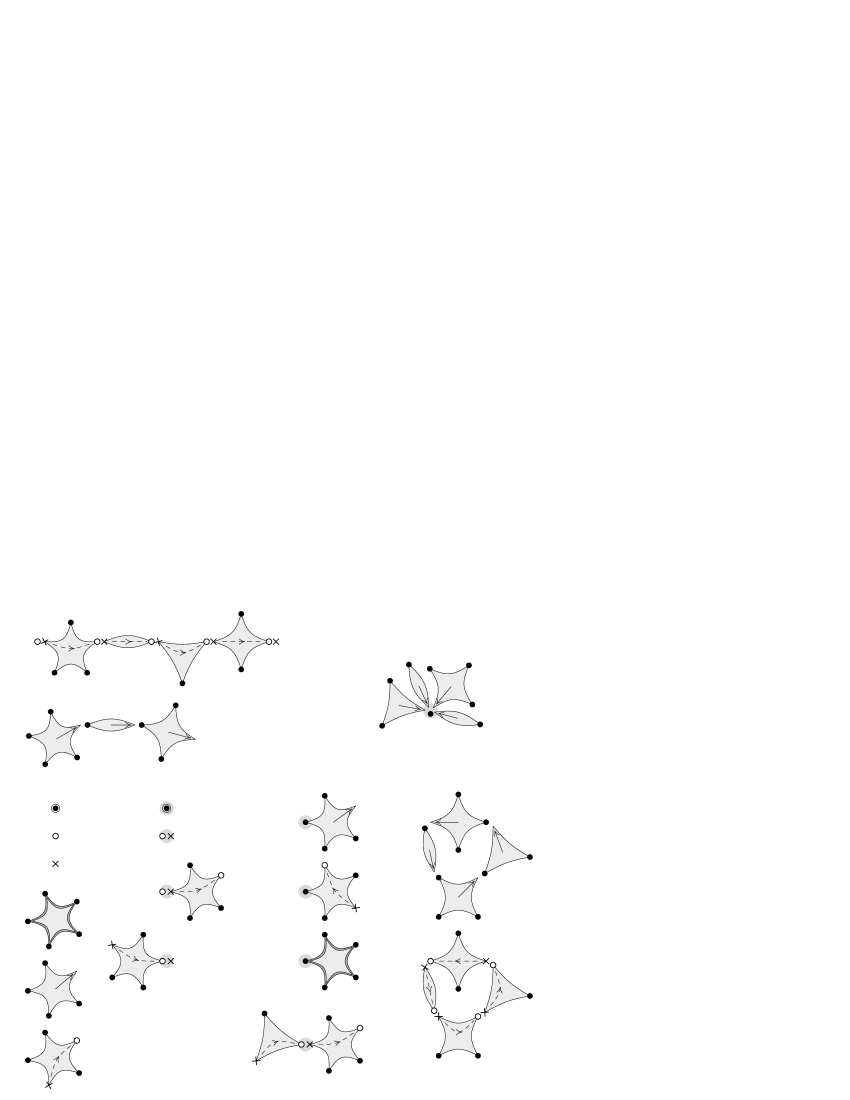
1b)		4b)
2)		4c)
3)		4d)

Figure 2: Possible ways of saturating the Grassmann fields on vertex $i$ (indicated by the small gray disk).

Having given the local description of the possible configurations at each vertex $i$, let us now describe the possible global configurations. Note first that at each vertex we can have at most two incident dashed arrows, and if there are two such arrows then they must have opposite orientations. As a consequence, we see that dashed arrows must either form cycles, or else form open paths connecting a source vertex of ${\sf I}\smallsetminus{\sf J}$ to a sink vertex of ${\sf J}\smallsetminus{\sf I}$. Let us use the term root structures to denote root vertices, root hyperedges, cycles of dashed hyperedges, and open paths of dashed hyperedges.

As for the solid arrows in the pointing hyperedges, the reasoning is as follows: If a pointing hyperedge $A$ points towards $i$, then either $i$ is part of a root structure as described above, or else it is a non-pointed vertex of another pointing hyperedge $\varphi(A)$. We can follow this map iteratively, i.e. go to $\varphi(\varphi(A))$, and so on:

Because of the finiteness of the graph, either we ultimately reach a root structure, or we enter a cycle. Cycles of the “dynamics” induced by $\varphi$ correspond to cycles of the pointing hyperedges. We now also include such cycles of pointing hyperedges as a fifth type of root structure (see Figure 3 for the complete list of root structures).

Figure 3: The five kinds of root structures.

All the rest is composed of pointing hyperedges, which form directed arborescences, rooted on the vertices of the root structures. In conclusion, therefore, the most general configuration consists of a bunch of disjoint root structures, and a set of directed arborescences (possibly reduced to a single vertex) rooted at its vertices, such that the whole is a spanning subhypergraph $H$ of $G$.

As each root structure is either a single vertex, a single hyperedge, a (hyper-)path or a (hyper-)cycle, we see that each connected component of $H$ is either a (hyper-)tree or a (hyper-)unicyclic. Furthermore, all vertices in ${\sf I}\cup{\sf J}$ are in the tree components, and each tree contains either one vertex from ${\sf I}$ and one from ${\sf J}$ (possibly coincident) or else no vertices at all from ${\sf I}\cup{\sf J}$.

We still need to understand the weights associated to the allowed configurations. Clearly, we have a factor $w_{A;i}$ per pointing hyperedge in the arborescence. Root vertices coming from $V^{\prime}$ have factors $t_{i}$, and root hyperedges have factors $\widehat{w}_{A}^{*}$. Cycles $\gamma=(i_{0},A_{1},i_{1},A_{2},....,i_{\ell}=i_{0})$ of the dynamics of $\varphi$ (bosonic cycles) have a weight $w_{A_{1};i_{1}}\cdots w_{A_{\ell};i_{\ell}}$. All the foregoing objects contain Grassmann variables only in the combination ${\bar{\psi}}_{i}\psi_{i}$, and hence are commutative. Finally, we must consider the dashed hyperedges, which contain “unpaired fermions” $\psi_{i}$ and ${\bar{\psi}}_{j}$, and hence will give rise to signs coming from anticommutativity. Let us first consider the dashed cycles $\gamma=(i_{0},A_{1},i_{1},A_{2},....,i_{\ell}=i_{0})$, and note what happens when reordering the fermionic fields:

$$(w_{A_{1};i_{\ell}i_{1}}\psi_{i_{\ell}}{\bar{\psi}}_{i_{1}})(w_{A_{2};i_{1}i_{2}}\psi_{i_{1}}{\bar{\psi}}_{i_{2}})\cdots(w_{A_{\ell};i_{\ell-1}i_{\ell}}\psi_{i_{\ell-1}}{\bar{\psi}}_{i_{\ell}})$$

$$\qquad=\;-w_{A_{1};i_{\ell}i_{1}}w_{A_{2};i_{1}i_{2}}\cdots w_{A_{\ell};i_{\ell-1}i_{\ell}}\,{\bar{\psi}}_{i_{1}}\psi_{i_{1}}\cdots{\bar{\psi}}_{i_{\ell}}\psi_{i_{\ell}}$$ (B.11)

because $\psi_{i_{\ell}}$ had to pass through $2\ell-1$ fermionic fields to reach its final location. This is pretty much the result one would have expected, but we have an overall minus sign, irrespective of the length of the cycle (or its parity), which is in a sense “non-local”, due to the fermionic nature of the fields $\psi$ and ${\bar{\psi}}$. For this reason we call a dashed cycle a fermionic cycle.

A similar mechanism arises for the open paths of dashed hyperedges $\gamma=(i_{0},A_{1},i_{1},$ $A_{2},\ldots,i_{\ell})$, where $i_{0}$ is the source vertex and $i_{\ell}$ is the sink vertex. Here the weight $w_{A_{1};i_{0}i_{1}}w_{A_{2};i_{1}i_{2}}\cdots w_{A_{\ell};i_{\ell-1}i_{\ell}}$ multiplies the monomial $\psi_{i_{0}}{\bar{\psi}}_{i_{1}}\psi_{i_{1}}{\bar{\psi}}_{i_{2}}\psi_{i_{2}}\cdots{\bar{\psi}}_{i_{\ell-1}}\psi_{i_{\ell-1}}{\bar{\psi}}_{i_{\ell}}$, in which the only unpaired fermions are $\psi_{i_{0}}$ and ${\bar{\psi}}_{i_{\ell}}$. in this order. Now the monomials for the open paths must be multiplied by ${\mathcal{O}}_{I,J}$, and each source (resp. sink) vertex from an open path must correspond to a vertex of ${\sf I}$ (resp. ${\sf J}$). This pairing thus induces a permutation of $\{1,\ldots,k\}$, where $k=|{\sf I}|=|{\sf J}|$: namely, $i_{r}$ is connected by an open path to $j_{\pi(r)}$. We then have

$$\Biggl{(}\prod_{r=1}^{k}{\bar{\psi}}_{i_{r}}\psi_{j_{r}}\Biggr{)}\Biggl{(}\prod_{r=1}^{k}\psi_{i_{r}}{\bar{\psi}}_{j_{\pi(r)}}\Biggr{)}\;,$$ (B.12)

where the first product is ${\mathcal{O}}_{I,J}$ and the second product comes from the open paths. This can easily be rewritten as

$$\prod_{r=1}^{k}{\bar{\psi}}_{i_{r}}\psi_{j_{r}}\psi_{i_{r}}{\bar{\psi}}_{j_{\pi(r)}}&=\prod_{r=1}^{k}{\bar{\psi}}_{i_{r}}\psi_{i_{r}}{\bar{\psi}}_{j_{\pi(r)}}\psi_{j_{r}}\\ =\Biggl{(}\prod_{r=1}^{k}{\bar{\psi}}_{i_{r}}\psi_{i_{r}}\Biggr{)}\Biggl{(}\prod_{r=1}^{k}{\bar{\psi}}_{j_{\pi(r)}}\psi_{j_{r}}\Biggr{)}\\ =\mathop{\rm sgn}\nolimits(\pi)\,\Biggl{(}\prod_{r=1}^{k}{\bar{\psi}}_{i_{r}}\psi_{i_{r}}\Biggr{)}\Biggl{(}\prod_{r=1}^{k}{\bar{\psi}}_{j_{r}}\psi_{j_{r}}\Biggr{)}\;.$$ (B.13)

Putting everything together, we see that the Grassmann integral (B.7) can be represented as a sum over rooted oriented spanning subhypergraphs $\vec{H}$ of $G$, as follows:

• Each connected component of $H$ (the unoriented subhypergraph corresponding to $\vec{H}$) is either a (hyper-)tree or a (hyper-)unicyclic.

• Each (hyper-)tree component contains either one vertex from ${\sf I}$ (the source vertex) and one from ${\sf J}$ (the sink vertex, which is allowed to coincide with the source vertex), or else no vertex from ${\sf I}\cup{\sf J}$. In the latter case, we choose either one vertex of the component to be the root vertex, or else one hyperedge of the component to be the root hyperedge.

• Each unicyclic component contains no vertex from ${\sf I}\cup{\sf J}$. As a unicyclic, it necessarily has the form of a single (hyper-)cycle together with (hyper-)trees (possibly reduced to a single vertex) rooted at the vertices of the (hyper-)cycle.

• Each hyperedge other than a root hyperedge is oriented by designating a vertex $i(A)\in A$ as the outgoing vertex. These orientations must satisfy following rules:

  • each (hyper-)tree component is directed towards the sink vertex, root vertex or root hyperedge,

  • each (hyper-)tree belonging to a unicyclic component is oriented towards the cycle, and

  • the (hyper-)cycle of each unicyclic component is oriented consistently.

  Thus, in each (hyper-)tree component the orientations are fixed uniquely, while in each unicyclic component we sum over the two consistent orientations of the cycle.

The weight of a configuration $\vec{H}$ is the product of the weights of its connected components, which are in turn defined as the product of the following factors:

• Each root vertex $i$ gets a factor $t_{i}$.

• Each root hyperedge $A$ gets a factor $\widehat{w}_{A}^{*}$.

• Each hyperedge $A$ belonging to the (unique) path from a source vertex to a sink vertex gets a factor $w_{A;ij}$, where $j$ is the outgoing vertex of $A$ and $i$ is the outgoing vertex of the preceding hyperedge along the path (or the source vertex if $A$ is the first hyperedge of the path).

• Each hyperedge $A$ that does not belong to a source-sink path or to a cycle gets a factor $w_{A;i(A)}$ [recall that $i(A)$ is the outgoing vertex of $A$].

• Each oriented cycle $(i_{0},A_{1},i_{1},A_{2},....,i_{\ell}=i_{0})$ gets a weight

  $$\prod_{\alpha=1}^{\ell}w_{A_{\alpha};i_{\alpha}}\,-\,\prod_{\alpha=1}^{\ell}w_{A_{\alpha};i_{\alpha-1}i_{\alpha}}\;.$$ (B.14)

• There is an overall factor $\mathop{\rm sgn}\nolimits(\pi)$.

B.2 Special cases

The contribution from unicyclic components cancels out whenever $\prod_{\alpha=1}^{\ell}w_{A_{\alpha};i_{\alpha}}=\prod_{\alpha=1}^{\ell}w_{A_{\alpha};i_{\alpha-1}i_{\alpha}}$ for every oriented cycle $(i_{0},A_{1},i_{1},A_{2},....,i_{\ell}=i_{0})$. In particular, this happens if $w_{A;ij}=w_{A;j}$ for all $A$ and all $i,j\in A$. More generally, it happens if $w_{A;ij}=w_{A;j}\exp(\phi_{A;ij})$ where $\phi$ has “zero circulation” in the sense that $\sum_{\alpha=1}^{\ell}\phi_{A_{\alpha};i_{\alpha-1}i_{\alpha}}=0$ for every oriented cycle $(i_{0},A_{1},i_{1},A_{2},....,i_{\ell}=i_{0})$. Physically, $\phi$ can be thought of as a kind of “gauge field’ to which the fermions $\psi,{\bar{\psi}}$ are coupled; the zero-circulation condition means that $\phi$ is gauge-equivalent to zero. Note, finally, that if $w_{A;i}w_{A;j}=w_{A;ij}w_{A;ji}$ for all $i,j\in A$, then $\widehat{w}_{A}^{*}=w_{A}^{*}$.

At the other extreme, if we take all $t_{i}=0$, all $\widehat{w}_{A}^{*}=0$ and $I=J=\varnothing$, then all tree components disappear, and we are left with only unicyclics.

In certain “symmetric” circumstances, we can combine the contributions from tree components having the same set of (unoriented) hyperedges but different roots, and obtain reasonably simple expressions. In particular, suppose that the weights $w_{A;i}$ are independent of $i$ (let us call them simply $w_{A}$), and consider a tree component $T$ that does not contain any vertices of ${\sf I}\cup{\sf J}$. Then we can sum over all choices of root vertex or root hyperedge, and obtain the weight

$$\Biggl{(}\prod_{A\in E(T)}w_{A}\Biggr{)}\Biggl{(}\sum_{i\in V(T)}t_{i}\,+\,\sum_{A\in E(T)}\frac{\widehat{w}_{A}^{*}}{w_{A}}\Biggr{)}\;.$$ (B.15)

A further simplification occurs in two cases:

• If all $t_{i}=t$ and all $\widehat{w}_{A}^{*}=0$, then the second factor in (B.15) becomes simply $t|V(T)|$: we obtain forests of vertex-weighted trees.

• If all $t_{i}=t$ and $\widehat{w}_{A}^{*}=t(1-|A|)w_{A}$ for all $A$, then the second factor in (B.15) becomes simply $t$ (by virtue of Proposition 2.1) and we obtain unrooted forests.

Recall, finally, that if we also take $w_{A;ij}=w_{A}$ for all $A$ and all $i,j\in A$, then the unicyclic components cancel and $\widehat{w}_{A}^{*}=w_{A}^{*}$, so that (B.15) reduces to (5.11).

It is instructive to consider the special case in which $G$ is an ordinary graph, i.e. each hyperedge $A\in E$ is of cardinality 2. If we further take all $w_{A}^{*}=0$, then the quantity in the exponential of the functional integral (B.7) is a quadratic form $\mathcal{S}(\psi,{\bar{\psi}})+\sum\limits_{i\in V}t_{i}{\bar{\psi}}_{i}\psi_{i}={\bar{\psi}}M\psi$, with matrix

$$M_{ij}\;=\;\begin{cases}t_{i}+\sum\limits_{k\neq i}w_{\{i,k\};k}&\hbox{if }i=j\\ -w_{\{i,j\};ji}&\hbox{if }i\neq j\end{cases}$$ (B.16)

Our result for $I=J=\varnothing$ then corresponds to the “two-matrix matrix-tree theorem” of Moon [5, Theorem 2.1] with $r_{ik}=w_{\{i,k\};k}$ for $i\neq k$, $r_{ii}=0$, $s_{ij}=w_{\{i,j\};ij}$ for $i\neq j$ and $s_{ii}=-t_{i}$.

References

- [1] G. Kirchhoff, Über die Auflösung der Gleichungen, auf welche man bei der Untersuchung der linearen Verteilung galvanischer Ströme gefuhrt wird, Ann. Physik Chemie, 72, 497–508 (1847).
- [2] R. L. Brooks, C. A. B. Smith, A. H. Stone and W. T. Tutte, The dissection of rectangles into squares, Duke Math. J. 7, 312–340 (1940).
- [3] A. Nerode and H. Shank, An algebraic proof of Kirchhoff’s network theorem, Amer. Math. Monthly 68, 244–247 (1961).
- [4] S. Chaiken, A combinatorial proof of the all minors matrix tree theorem, SIAM J. Alg. Disc. Meth., 3, 319–329 (1982).
- [5] J. W. Moon, Some determinant expansions and the matrix-tree theorem, Discrete Math. 124, 163–171 (1994).
- [6] A. Abdesselam, Grassmann–Berezin calculus and theorems of the matrix-tree type, Adv. Appl. Math. 33, 51–70 (2004), math.CO/0306396 at arXiv.org.
- [7] N. Balabanian and T.A. Bickart, Electrical Network Theory (Wiley, New York, 1969).
- [8] W. K. Chen, Applied Graph Theory: Graphs and Electrical Networks, 2nd ed. (North-Holland, New York, 1976).
- [9] B. Duplantier and F. David, Exact partition functions and correlation functions for multiple hamiltonian walks on the Manhattan lattice, J. Stat. Phys. 51, 327–434 (1988).
- [10] F.Y. Wu, Dimers and spanning trees: some recent results, Int. J. Mod. Phys. B 16, 1951–1961 (2002).
- [11] F. A. Berezin, Introduction to Superanalysis (Reidel, Dordrecht, 1987).
- [12] S. Caracciolo, J. L. Jacobsen, H. Saleur, A. D. Sokal, A. Sportiello, Fermionic field theory for trees and forests, Phys. Rev. Lett. 93, 080601 (2004), cond-mat/0403271 at arXiv.org.
- [13] G. Masbaum and A. Vaintrob, A new matrix-tree theorem, Int. Math. Res. Not., no. 27, 1397–1426 (2002).
- [14] G. Masbaum and A. Vaintrob, Milnor numbers, spanning trees, and the Alexander-Conway polynomial, Adv. Math. 180, 765–797 (2003), math.GT/0111102 at arXiv.org.
- [15] S. Hirschman and V. Reiner, Note on the Pfaffian-tree theorem, Graphs Combin. 20, 59–63 (2004).
- [16] M.J. Stephen, Percolation problems and the Potts model, Phys. Lett. A 56, 149–150 (1976).
- [17] F.Y. Wu, Number of spanning trees on a lattice, J. Phys. A: Math. Gen. 10, L113–L115 (1977).
- [18] J. L. Jacobsen, J. Salas and A. D. Sokal, Spanning forests and the q-state Potts model in the limit , J. Stat. Phys. 119, 1153 (2005), cond-mat/0401026 at arXiv.org.
- [19] A. D. Sokal, The multivariate Tutte polynomial (alias Potts model) for graphs and matroids, in Surveys in Combinatorics, 2005, edited by Bridget S. Webb (Cambridge University Press, Cambridge, 2005), pp. 173–226, math.CO/0503607 at arXiv.org.
- [20] S. Caracciolo, C. De Grandi and A. Sportiello, Renormalization flow for unrooted forests on a triangular lattice, Nucl. Phys. B (2007), doi:10.1016/j.nuclphysb.2007.06.012, arXiv:0705.3891 at arXiv.org.
- [21] R. Diestel, Graph Theory, 3rd ed. (Springer-Verlag, New York, 2005).
- [22] C. Berge, Graphs and Hypergraphs (North-Holland, Amsterdam, 1973).
- [23] C. Berge, Hypergraphs: Combinatorics of Finite Sets (North-Holland, Amsterdam, 1989).
- [24] G. Grimmett, Potts models and random-cluster processes with many-body interactions, J. Stat. Phys. 75, 67–121 (1994).
- [25] F. Ricci-Tersenghi, M. Weigt and R. Zecchina, Simplest random K-satisfiability problem, Phys. Rev. E 63, 026702 (2001), cond-mat/0011181 at arXiv.org.
- [26] S. Caracciolo and A. Sportiello, An exactly solvable random satisfiability problem, J. Phys. A: Math. Gen. 35, 7661–7688 (2002), cond-mat/0206352 at arXiv.org.
- [27] T. Castellani, V. Napolano, F. Ricci-Tersenghi and R. Zecchina, Bicolouring random hypergraphs, J. Phys. A: Math. Gen. 36, 11037–11053 (2003), cond-mat/0306369 at arXiv.org.
- [28] J. Zinn-Justin, Quantum Field Theory and Critical Phenomena, 3rd ed. (Clarendon Press, Oxford, 1996).
- [29] L.D. Andersen and H. Fleischner, The NP-completeness of finding A-trails in Eulerian graphs and of finding spanning trees in hypergraphs, Discrete Appl. Math. 59, 203–214 (1995).
- [30] S. Caracciolo, A. D. Sokal and A. Sportiello, Spanning forests, -invariant -models, and -invariant -models at , in preparation.
- [31] S. Caracciolo, A. D. Sokal and A. Sportiello, Ward identities and combinatorial identities in -invariant models describing spanning (hyper)forests, in preparation.
- [32] S. Caracciolo, A. Sportiello, M. Polin and A. D. Sokal, Combinatorial proofs of Cayley-type identities for derivatives of determinants and pfaffians, in preparation.
- [33] J. McCammond and J. Meier, The hypertree poset and the -Betti numbers of the motion group of the trivial link, Math. Ann. 328, 633–652 (2004).
- [34] I.M. Gessel and L.H. Kalikow, Hypergraphs and a functional equation of Bouwkamp and de Bruijn, J. Combin. Theory A 110, 275–289 (2005).
- [35] P.W. Kasteleyn and C.M. Fortuin, Phase transitions in lattice systems with random local properties, J. Phys. Soc. Japan 26 (Suppl.), 11–14 (1969).
- [36] C.M. Fortuin and P.W. Kasteleyn, On the random-cluster model. I. Introduction and relation to other models, Physica 57, 536–564 (1972).
- [37] R.P. Stanley, Enumerative Combinatorics, vol. 1 (Wadsworth & Brooks/Cole, Monterey, California, 1986). Reprinted by Cambridge University Press, 1997.
- [38] N.G. De Bruijn, Asymptotic Methods in Analysis, 2nd ed. (North-Holland, Amsterdam, 1961).
- [39] S. Caracciolo, A. D. Sokal and A. Sportiello, Algebraic properties of a Grassmann subalgebra related to spanning hyperforests, in preparation.
- [40] A. Bedini, S. Caracciolo, A.D. Sokal and A. Sportiello, Counting spanning hyperforests in the complete -uniform hypergraph by Grassmann integral representation, in preparation.
- [41] V. Rittenberg, A guide to Lie superalgebras, in Group Theoretical Methods in Physics, Lecture Notes in Physics #79 (Springer-Verlag, Berlin–New York, 1978), pp. 3–21.
- [42] M. Scheunert, The Theory of Lie Superalgebras, Lecture Notes in Mathematics #716 (Springer-Verlag, Berlin, 1979).
- [43] F.A. Berezin and V.N. Tolstoy, The group with Grassmann structure , Commun. Math. Phys. 78, 409–428 (1981).
- [44] P. Lancaster and M. Tismenetsky, The Theory of Matrices, 2nd ed. (Academic Press, London–New York–Orlando, 1985).
- [45] M. Marcus, Finite Dimensional Multilinear Algebra, Part 2 (Marcel Dekker, New York, 1975).
- [46] V.E. Korepin, N.M. Bogoliubov and A.G. Izergin, Quantum Inverse Scattering Method and Correlation Functions (Cambridge University Press, Cambridge–New York, 1993).
- [47] S.M. Rump, Theorems of Perron–Frobenius type for matrices without sign restrictions, Lin. Alg. Appl. 266, 1–42 (1997).
- [48] U. Prells, M.I. Friswell and S.D. Garvey, Use of geometric algebra: Compound matrices and the determinant of the sum of two matrices, Proc. Roy. Soc. London A 459, 273–285 (2003).
- [49] A.C. Aitken, Determinants and Matrices, 5th ed. (Oliver and Boyd, Edinburgh–London, 1948).