Longitudinal Shower Profile Reconstruction from Fluorescence and Cherenkov Light

Abstract

Traditionally, longitudinal shower profiles are reconstructed in fluorescence light experiments by treating the Cherenkov light contribution as background. Here we will argue that, due to universality of the energy spectra of electrons and positrons, both fluorescence and Cherenkov light can be used simultaneously as signal to infer the longitudinal shower development. We present a new profile reconstruction method that is based on the analytic least-square solution for the estimation of the shower profile from the observed light signal and discuss the extrapolation of the profile with a Gaisser-Hillas function.

1 Introduction

During its passage through the atmosphere of the earth an extensive air shower excites nitrogen molecules of the air, which subsequently radiate isotropically ultraviolet fluorescence light. Since the amount of emitted light is proportional to the energy deposited, the longitudinal shower development can be observed by appropriate optical detectors such as HiRes [1], Auger [2] or TA [3].
As part of the charged shower particles travel faster than the speed of light in air, Cherenkov light is emitted in addition. Therefore, in general a mixture of the two light sources reaches the aperture of the detector.
In the traditional method [4] for the reconstruction of the longitudinal shower development the Cherenkov light is iteratively subtracted from the measured total light. The drawbacks of this ansatz are the lack of convergence for events with a large amount of Cherenkov light and the difficulty of propagating the uncertainty of the subtracted signal to the reconstructed shower profile.
It has already been noted in [5] that, due to the universality of the energy spectra of the secondary electrons and positrons within an air shower, there exists a non-iterative solution for the reconstruction of a longitudinal shower profile from light detected by fluorescence telescopes.
Here we will present the analytic least-square solution for the estimation of the shower profile from the observed light signal in which both, fluorescence and Cherenkov light, are treated as signal.

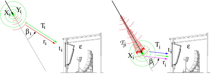
Figure 1: Illustration of the isotropic fluorescence light emission (circles), Cherenkov beam along the shower axis and the direct (left) and scattered (right) Cherenkov light contributions.

2 Scattered and Direct Light

The non-scattered, i.e. direct fluorescence light emitted at a certain slant depth $X_{i}$ is measured at the detector at a time $t_{i}$. Given the fluorescence yield $Y^{\mathrm{f}}_{i}$ [6, 7] at this point of the atmosphere, the number of photons produced at the shower in a slant depth interval $\Delta X_{i}$ is

$$N_{\gamma}^{\mathrm{f}}(X_{i})=Y^{\mathrm{f}}_{i}\,w_{i}\,\Delta X_{i},$$

where $w_{i}$ denotes the energy deposited at slant depth $X_{i}$ (cf. Fig. 1). These photons are distributed over a sphere with surface $4\,\pi\,r_{i}^{2}$, where $r_{i}$ denotes the distance of the detector. Due to atmospheric attenuation only a fraction $T_{i}$ of them can be detected. Given a light detection efficiency of $\varepsilon$, the measured fluorescence light flux $y_{i}^{\mathrm{f}}$ can be written as

$$y_{i}^{\mathrm{f}}=d_{i}\,Y^{\mathrm{f}}_{i}\,w_{i}\,\Delta X_{i},$$ (1)

where the abbreviation $d_{i}=\frac{\varepsilon\,T_{i}}{4\,\pi\,r_{i}^{2}}$ was used. For the sake of clarity the wave length dependence of $Y$, $T$ and $\varepsilon$ will be disregarded in the following but be discussed later.
The number of Cherenkov photons emitted at the shower is proportional to the number of charged particles above the Cherenkov threshold energy. Since the electromagnetic component dominates the shower development, the emitted Cherenkov light, $N_{\gamma}^{\mathrm{C}}$, can e calculated from

$$N_{\gamma}^{\mathrm{C}}(X_{i})=Y^{\mathrm{C}}_{i}\,N^{\mathrm{e}}_{i}\,\Delta X_{i},$$

where $N^{\mathrm{e}}_{i}$ denotes the number of electrons and positrons above a certain energy cutoff, which is constant over the full shower track and not to be confused with the Cherenkov emission energy threshold. Details of the Cherenkov light production like these thresholds are included in the Cherenkov yield factor $Y^{\mathrm{C}}_{i}$ [5, 8, 9, 10].

Although the Cherenkov photons are emitted in a narrow cone along the particle direction, they cover a considerable angular range with respect to the shower axis, because the charged particles are deflected from the primary particle direction due to multiple scattering. Given the fraction $f_{\mathrm{C}}(\beta_{i})$ of Cherenkov photons emitted at an angle $\beta_{i}$ with respect to the shower axis [8, 10], the light flux at the detector aperture originating from direct Cherenkov light is

$$y_{i}^{\mathrm{Cd}}=d_{i}\,f_{\mathrm{C}}(\beta_{i})\,Y^{\mathrm{C}}_{i}\,\Delta X_{i}\,N^{\mathrm{e}}_{i}.$$ (2)

Due to the forward peaked nature of Cherenkov light production, an intense Cherenkov light beam can build up along the shower as it traverses the atmosphere (cf. Fig. 1). If a fraction $f_{\mathrm{s}}(\beta_{i})$ of the beam is scattered towards the detector it can contribute significantly to the total light received. In a simple one-dimensional model the number of photons in the beam at depth $X_{i}$ is just the sum of Cherenkov light produced at all previous depths $X_{j}$ attenuated on the way from $X_{j}$ to $X_{i}$ by $\mathcal{T}_{ji}$:

$$N_{\gamma}^{\mathrm{beam}}(X_{i})=\sum_{j=0}^{i}\mathcal{T}_{ji}\,Y^{\mathrm{C}}_{j}\,\Delta X_{j}\,N^{\mathrm{e}}_{j}.$$

Similar to the direct contributions, the scattered Cherenkov light received at the detector is then

$$y_{i}^{\mathrm{Cs}}=d_{i}\,f_{\mathrm{s}}(\beta_{i})\,\sum_{j=0}^{i}\mathcal{T}_{ji}\,Y^{\mathrm{C}}_{j}\,\Delta X_{j}\,N^{\mathrm{e}}_{j}.$$ (3)

Finally, the total light received at the detector at the time $t_{i}$ is obtained by adding the scattered and direct light contributions.

3 Shower Profile Reconstruction

The aim of the profile reconstruction is to estimate the energy deposit and/or electron profile from the light flux observed at the detector. At first glance this seems to be hopeless, since at each depth there are the two unknown variables $w_{i}$ and $N^{\mathrm{e}}_{i}$, and only one measured quantity, namely $y_{i}$. Since the total energy deposit is just the sum of the energy loss of electrons, $w_{i}$ and $N^{\mathrm{e}}_{i}$ are related via

$$w_{i}=N^{\mathrm{e}}_{i}\,\int_{0}^{\infty}f_{\mathrm{e}}(E,X_{i})\;w_{\mathrm{e}}(E)\;\mathrm{d}E,$$ (4)

where $f_{\mathrm{e}}(E,X_{i})$ denotes the normalized electron energy distribution and $w_{\mathrm{e}}(E,X_{i})$ is the energy loss of a single electron with energy $E$. As it is shown in [9, 5, 10], the electron energy spectrum $f_{\mathrm{e}}(E,X_{i})$ is universal in shower age $s_{i}=3/(1+2X_{\mathrm{max}}/X_{i})$, i.e. it does not depend on the primary mass or energy, but only on the relative distance to the shower maximum, $X_{\mathrm{max}}$. Eq. (4) can thus be simplified to

$$w_{i}=N^{\mathrm{e}}_{i}\;\alpha_{i}.$$

where $\alpha_{i}$ is the average energy deposit per electron at shower age $s_{i}$. With this one-to-one relation between the energy deposit and the number of electrons, the shower profile is readily calculable from the equations given in the last section. For the solution of the problem, it is convenient to rewrite the relation between energy deposit and light at the detector in matrix notation: Let $\mathbf{y}=(y_{1},y_{2},\dots,y_{n})^{\mathrm{T}}$ be the $n$-component vector (histogram) of the measured photon flux at the aperture and $\mathbf{w}=(w_{1},w_{2},\dots,w_{n})^{\mathrm{T}}$ the energy deposit vector at the shower track. Using the ansatz

$$\mathbf{y}=\mathbf{C}\cdot\mathbf{w}$$ (5)

the elements of the Cherenkov-fluorescence matrix $\mathbf{C}$ can be found by a comparison with the coefficients in equations (1), (2) and (3):

$$C_{ij}=\begin{cases}0,\hfill i<j\!\;\\ c_{i}^{\mathrm{d}}+c_{ii}^{\mathrm{s}},\;\;\;i=j\,\\ c_{ij}^{\mathrm{s}},\hfill i>j,\\ \end{cases}$$ (6)

where

$$c_{i}^{\mathrm{d}}=d_{i}\left(Y^{\mathrm{f}}_{i}+f_{\mathrm{C}}(\beta_{i})\,Y^{\mathrm{C}}_{i}/\alpha_{i}\right)\,\Delta X_{i}$$

and

$$c_{ij}^{\mathrm{s}}=d_{i}\,f_{\mathrm{s}}(\beta_{i})\,\mathcal{T}_{ji}\,Y^{\mathrm{C}}_{j}/\alpha_{j}\,\Delta X_{j}.$$

The solution of Eq. (5) can be obtained by inversion, leading to the energy deposit estimator $\widehat{\mathbf{w}}$:

$$\widehat{\mathbf{w}}=\mathbf{C}^{-1}\cdot\mathbf{y}\,.$$

Due to the triangular structure of the Cherenkov-fluorescence matrix the inverse can be calculated fast even for matrices with large dimension. As the matrix elements in (6) are always $\geq 0$, $\mathbf{C}$ is never singular.
The statistical uncertainties of $\widehat{\mathbf{w}}$ are obtained by error propagation:

$$\mathbf{V_{w}}=\mathbf{C}^{-1}\,\mathbf{V_{y}}\left(\mathbf{C}^{\mathrm{T}}\right)^{-1}\;.$$

It is interesting to note that even if the measurements $y_{i}$ are uncorrelated, i.e. their covariance matrix $\mathbf{V_{y}}$ is diagonal, the calculated energy loss values $\widehat{w}_{i}$ are not. This is, because the light observed during time interval $i$ does not solely originate from $w_{i}$, but also receives a contribution from earlier shower parts $w_{j}$, $j<i$, via the ’Cherenkov beam’.

4 Wavelength Dependence

Until now it has been assumed that the shower induces light emission at a single wavelength $\lambda$. In reality, the fluorescence yield shows distinct emission peaks and the number of Cherenkov photons is proportional to $\frac{1}{\lambda^{2}}$. In that case, also the wavelength dependence of the detector efficiency and the light transmission need to be taken into account. Assuming that a binned wavelength distribution of the yields is available ($Y_{ik}=\int_{\lambda_{k}-\Delta\lambda}^{\lambda_{k}+\Delta\lambda}Y_{i}(\lambda)\,\mathrm{d}\lambda$), the above considerations still hold when replacing $c_{i}^{\mathrm{d}}$ and $c_{ij}^{\mathrm{s}}$ in Eq. (6) by

$$\tilde{c}_{i}^{\mathrm{\,d}}=\Delta X_{i}\sum_{k}\,d_{ik}\left(Y^{\mathrm{f}}_{ik}+f_{\mathrm{C}}(\beta_{i})\,Y^{\mathrm{C}}_{ik}/\alpha_{i}\right)$$

and

$$\tilde{c}_{ij}^{\mathrm{\,s}}=\Delta X_{j}\sum_{k}\,d_{ik}\,f_{\mathrm{s}}(\beta_{i})\,\mathcal{T}_{jik}\,Y^{\mathrm{C}}_{jk}/\alpha_{j},$$

where

$$d_{ik}=\frac{\varepsilon_{k}\,T_{ik}}{4\,\pi\,r_{i}^{2}}.$$

The detector efficiency $\varepsilon_{k}$ and transmission coefficients $T_{ik}$ and $\mathcal{T}_{jik}$ are evaluated at the wavelength $\lambda_{k}$.

5 Shower Age Dependence

Due to the age dependence of the electron spectra $f_{\mathrm{e}}(E,s_{i})$, the Cherenkov yield factors $Y^{\mathrm{C}}_{i}$ and the average electron energy deposits $\alpha_{i}$ depend on the shower maximum, which is not known before the profile has been reconstructed. Fortunately, these dependencies are small: In the age range of importance for the shower profile reconstruction ($s\in[0.8,1.2]$) $\alpha$ varies only within a few percent [10] and $Y^{\mathrm{C}}$ by less than 15% [5]. Therefore, a good estimate of $\alpha$ and $Y^{\mathrm{C}}$ can be obtained by setting $s=1$. After the shower profile has been calculated with these estimates, $X_{\mathrm{max}}$ can be determined and the profiles can be re-calculated with an updated Cherenkov-fluorescence matrix.

6 Gaisser-Hillas Fit

The knowledge of the complete profile is required for the calculation of the Cherenkov beam and the shower energy. If due to the limited field of view of the detector only a part of the profile is observed, an appropriate function for the extrapolation to unobserved depths is needed. A possible choice is the Gaisser-Hillas function [11] which was found to give a good description of measured longitudinal profiles [12]. It has only four free parameters: $X_{\mathrm{max}}$, the depth where the shower reaches its maximum energy deposit $w_{\mathrm{max}}$ and two shape parameters $X_{0}$ and $\lambda$.
The best set of Gaisser-Hillas parameters $\mathbf{p}$ can be obtained by minimizing the error weighted squared difference between the vector of function values $\mathbf{f_{\mathrm{GH}}}$ and $\widehat{\mathbf{x}}$, which is

$$\chi^{2}_{\mathrm{GH}}=\left[\,\widehat{\mathbf{w}}-\mathbf{f(\mathbf{p})}\right]^{\mathrm{T}}\,\mathbf{V_{w}}^{\!\!\!-1}\,\left[\,\widehat{\mathbf{w}}-\mathbf{f(\mathbf{p})}\right]$$

This minimization works well if a large fraction of the shower has been observed below and above the shower maximum. If this is not the case, or even worse, if the shower maximum is outside the field of view, the problem is under-determined, i.e. the experimental information is not sufficient to reconstruct all four Gaisser-Hillas parameters. This complication can be overcome by weakly constraining $X_{0}$ and $\lambda$ to their average values $\langle X_{0}\rangle$ and $\langle\lambda\rangle$. The new minimization function is then the modified $\chi^{2}$

$$\chi^{2}=\chi^{2}_{\mathrm{GH}}+\frac{(X_{0}-\langle X_{0}\rangle)^{2}}{V_{X_{0}}}+\frac{(\lambda-\langle\lambda\rangle)^{2}}{V_{\lambda}}\,,$$

where the variance of $X_{0}$ and $\lambda$ around their mean values are in the denominators.
In this way, even if $\chi^{2}_{\mathrm{GH}}$ is not sensitive to $X_{0}$ and $\lambda$, the minimization will still converge. On the other hand, if the measurements have small statistical uncertainties and/or cover a wide range in depth, the minimization function is flexible enough to allow for shape parameters differing from their mean values. These mean values can be determined from air shower simulations or, preferably, from high quality data profiles which can be reconstructed without constraints.

References

- [1] T. Abu-Zayyad et al. [HiRes Collaboration]. Nucl. Instrum. Meth., A450:253, 2000.
- [2] J. Abraham et al. [Pierre Auger Collaboration]. Nucl. Instrum. Meth., A523:50, 2004.
- [3] H. Kawai et al. [Telescope Array Collaboration]. Proc. 29th ICRC, 8:141, 2005.
- [4] R. M. Baltrusaitis et al. [Fly’s Eye Collaboration]. Nucl. Instrum. Meth., A240:410, 1985.
- [5] M. Giller et al. J. Phys. G, 30:97, 2004.
- [6] M. Nagano et al. Astropart. Phys., 22:235, 2004.
- [7] F. Kakimoto et al. Nucl. Instrum. Meth., A372:527, 1996.
- [8] A. M. Hillas. J. Phys. G, 8:1461, 1982.
- [9] A. M. Hillas. J. Phys. G, 8:1475, 1982.
- [10] F. Nerling et al. Astropart. Phys., 24:421, 2006.
- [11] T. K. Gaisser and A. M. Hillas. Proc. 15th ICRC, 8:353, 1977.
- [12] Z. Cao et al. [HiRes Collaboration]. Proc. 28th ICRC, page 378, 2003.