Heterogeneity and Increasing Returns May Drive Socio-Economic Transitions

Abstract

There are clear benefits associated with a particular consumer choice for many current markets. For example, as we consider here, some products might carry environmental or ‘green’ benefits. Some consumers might value these benefits while others do not. However, as evidenced by myriad failed attempts of environmental products to maintain even a niche market, such benefits do not necessarily outweigh the extra purchasing cost. The question we pose is, how can such an initially economically-disadvantaged green product evolve to hold the greater share of the market? We present a simple mathematical model for the dynamics of product competition in a heterogeneous consumer population. Our model preassigns a hierarchy to the products, which designates the consumer choice when prices are comparable, while prices are dynamically rescaled to reflect increasing returns to scale. Our approach allows us to model many scenarios of technology substitution and provides a method for generalizing market forces. With this model, we begin to forecast irreversible trends associated with consumer dynamics as well as policies that could be made to influence transitions.

1 Introduction

The adoption of ‘green’ technology is hard to predict because it implies many intertwined social and economic factors plus many retro-action loops. Because even a partial description of these factors and their interaction seems so intricate, authors are attracted by the multi-agent modelling approach (see, e.g., [2] and the related special issue of JASSS). But this approach suffers many limitations, especially when it comes to obtain a full description of the dynamics in the parameter space or to get some insight in what happens in the model and how it can be compared to the real modelled system. This is especially important because one might observe sharp changes in predictions in very small areas of the parameter space (see also [7]).

We here propose a simple soluble model that takes into account some of the intricacies of real life problems such as the heterogeneity in consumer responses, social influence, and increasing returns to scale of production prices but still condenses the set of parameters that can lead to unwieldy complexity in simulation (see also [5] for a related model, but without increasing returns to scale). The increasing returns to scale could also be interpreted as increasing social pressure to buy a specific product if most people around you do this, an argument already made by B. Arthur[1] . To maintain our analysis on the competition between goods with different prices and different levels of environmental soundness, we subsume that the influences of different cultures, social influences, government policy, advertising can all be summarized into a single curve, which we name the ‘willingness to pay’ (WTP) function. WTP illuminates the consumer population distribution as a function of price and describes how people vary in their extent to which they want to pay for environmental benefits. We assume this normalized WTP distribution has a fixed shape, while the price associated with each market product varies with its market share.

Our model has three ancillary assumptions. Firstly, given that there are two products with prices below what a consumer is willing to pay, this consumer chooses the ‘greener’ technology. The first assumption implies that we can assume without further loss of generality also that environmentally superior technologies are more expensive given a similar market share. Given the first assumption, products that are more expensive and less ‘green’ cannot survive in this market. Secondly, prices decrease with market shares. The combination of buyers heterogeneity in WTP and increasing returns results in a rich variety of dynamical regimes with ultimately different prices and market shares. Thirdly, we assume that while each product varies in maximum price, they each experience a similar extent of linear decreasing returns to scale. This last assumption could very easily be relaxed in future extensions of the model, but is not crucial for the implications we derive in this paper.

In our investigation we focus our attention on a market competition between three cars: a standard (0), hybrid (1), ‘green’ (2). Figure 1 shows a bell-shaped WTP distribution where the prices associated with each car, $p_{0}$, $p_{1}$, and $p_{2}$ determine the corresponding market share areas, $u_{0}$, $u_{1}$, and $u_{2}$, shaded in red, blue, and green, respectively. Consumers with WTP larger than $p_{2}$ choose car 2. Of the remaining market share, consumers with WTP larger than $p_{1}$ choose car 1. Finally, from the still remaining market share, consumers with WTP larger than $p_{0}$ choose car 0. According to the WTP distribution, some agents might decide to buy no car so that $u_{0}+u_{1}+u_{2}\leq 1$.

This paper is organized as follows. Section 2 describes our computational model with equations. Section 3 describes our results. We show that environmental technologies will take over when a significant fraction of agents have already a WTP to pay for the green car whatever its market share and when the increasing returns coefficient is large (because of strong social effects or large production price reduction with production level). We also demonstrate how different conditions can lead to car 0, 1, or 2 dominating the market depending on the rescaling of price due to demand. Subsection 3.2 shows that our simple model not only provides reliable results but also analytic tools to evaluate multiple asymptotic solutions. For some parameter values, the dynamics have several attractors, which implies hysteresis effects. We extrapolate that the timing of the subsidies and grants at the immediate onset or emergence of a new technology may be crucial as trends are sometimes irreversible. Section 4 summarizes our conclusions and shows future direction for this model.

2 A Simple Set of Assumptions

We start the description of our model with explaining in more detail our assumptions. We use the example of more or less green cars below, but clearly any product for which there is some non-monetary benefit related to the product can be used instead. So where we write for convenience ‘car’ below, one could read ‘product,’ and when we write environmental benefits or ‘greenness,’ one could read more non-monetary benefits (ammenities).

• Consumers care about two aspects of a car, i.e., the price and ‘greenness’ of the car;

• Environmentally superior technologies are more expensive (given a similar market share);

• Cars with a larger market share are cheaper;

• People vary in their extent to which they want to pay for environmental benefits (heterogeneity of WTP) [3, 4, 6]

• People choose the alternative they prefer.

The second assumption is more for convenience than that it is really necessary. Environmentally inferior technologies that are more expensive would not be chosen by anybody, because consumers only care about these two aspects.

The third assumption has also two possible interpretations. A larger market share has advantages of scale for the producers, which implies that cars can be produced for a lower price when the market share is larger. From the buyers perspective, social influence effects affect the utility consumers get from a product: a more popular car is more attractive for most individuals than a car that nobody bought, which changes the specific willingness to pay for that type of car. But this is equivalent to saying that the price of that type of car decreases. Since only the difference between WTP and prices is relevant to buyers’ decisions, both effects have the same results [1]. In theory one should make a distinction between the production costs which are influenced by market shares say during the actual year, and the social influence terms which takes into account how many cars of each type have been bought in the past (the integrated yearly market share). In practice, because of the irreversibility of the capital investment in the automobile industry, the actual production cost also integrate investments and the two effects are driven by the integrated market share.

There are three technological options: standard (0), intermediate (1), ‘green’ (2).

• Each option $i$ has its own maximum cost $P_{0i}$, which equals the cost at a zero market share;

• All options have the same linear returns to scale coefficient $k$ (i.e., $p_{i}=P_{0i}-ku_{i}$, where $p_{i}$ and $u_{i}$ are the actual price and market share of product $i$, respectively;)

• There is one distribution of WTP for environmental benefits (e.g., uniform or bell-shaped)

Figure 1: Distribution of willingness to pay (WTP) and market shares. Consumers with WTP larger than $p_{i}$ may choose car $i$ with market share $u_{i}$ equal to the colored area.

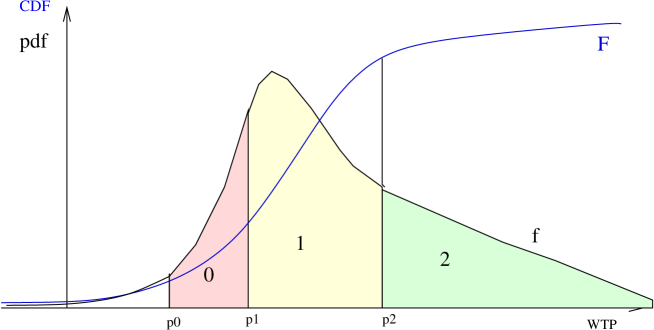
Figure 1 shows an arbitrary distribution of WTP. Consumers with WTP larger than $p_{i}$ may choose car $i$ with market share $u_{i}$ equal to the colored area. In the following subsection, we explain how the stable market shares are computed.

2.1 Equations

Given that we assume the same returns to scale, the price of a product follows a linear return to scale function.

$$p_{i}=P_{0i}-ku_{i}$$ (1)

Because of the influence of market share on actual prices, the order among actual prices $p_{i}$ may differ from maximum prices at zero market share. A first operation is to order products $i$. New indices $j$ are used for prices ordered by increasing actual prices, according to market share distribution. Some products might lose their rank: in such a case, we consider that every time a product $j$ has larger price $p_{j}$ than a product with a better environmental quality, it disappears from the market: nobody is interested to buy a more expensive product with a lower environmental quality. With final indices $j$, equilibrium market shares obey:

$$u_{j}=F(p_{j+1})-F(p_{j})$$ (2)

where $F(p)$ is the cumulative WTP distribution. This simple set of equations is soluble, either directly for simple expressions of $F(p)$, as we do in section 3.2 on results or through transcendental equations.

While these equations provide the (possible multiple) solutions for the stable proportions of each product in the market, one can also simulate the dynamics to these solution by assuming that at each point in time a certain proportion $\lambda$ of consumers is choosing a new car according to the prices and preferences at that point in time. The related dynamics of market shares is given by:

$$u_{j}(t+1)=(1-\lambda)u_{j}(t)+\lambda(F(p_{j+1},t)-F(p_{j},t))$$ (3)

Figure 2: Distributions of willingness to pay (WTP). A uniform partial distribution function (pdf) and the corresponding cumulative distribution function (cdf) are drawn in black. The corresponding logit distributions are drawn in red (bell-shaped for the pdf, S-shaped for the cdf).

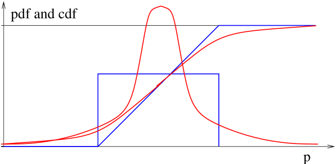
The simulations in this paper were done for two simple WTP distributions: the uniform distribution and a logit distribution. The corresponding equation for the cumulative distribution $F(p)$ is piecewise linear for the uniform distribution:

$$F(p)=\frac{p-p_{m}}{p_{M}-p_{m}}$$ (4)

between the minimum $p_{m}$ and the maximum $p_{M}$ WTP price. Below $p_{m}$, $F(p)=0$, above $p_{M}$, $F(p)=1$.

For the bell-shaped cumulative distribution we use a logit expression:

$$F(p)=\frac{1}{1+exp(-\beta p)}$$ (5)

where $\beta$ is inversely proportional to the width of the distribution. If we define the width as the inverse slope at the point of inflexion ($p=0$), we obtain:

$$w=\frac{4}{\beta}.$$ (6)

The corresponding graphs appear in figure 2.

3 Results

3.1 Time evolution of market shares

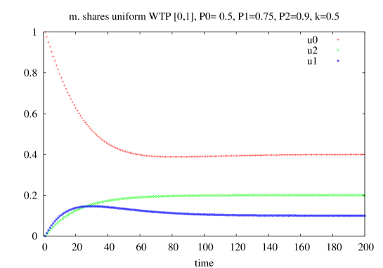
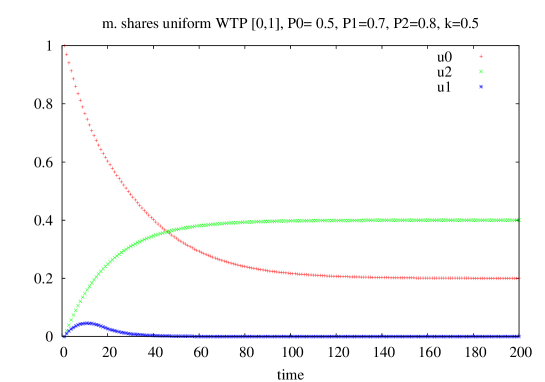
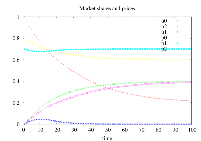
The evolution of market shares for the three products is easily simulated for a fixed set of parameters. The two plots of figure 3 only differ by the value of the maximum price of the green product $P_{02}$. In both cases, as in most simulations, only the standard product is initially present ($u_{0}(t=0)=1,u_{1}(0)=0,u_{2}(0)=0$). This corresponds with the assumption that we want to predict at which maximum prices it is possible to enter the market for greener products.

Asymptotic market shares are reached in a few characteristic times $(\lambda)^{-1}$, where $(\lambda)^{-1}$ corresponds to a minimum characteristic time of evolution towards equilibrium.

The connection between the evolution of market shares and prices is evident from figure 4, obtained for the same parameter values as the right plot of figure 3. The initial increase of $u_{1}$ and $u_{2}$ decreases $u_{0}$, $p_{1}$, and $p_{2}$, and increases $p_{0}$. Since $p_{1}$ decreases slower than $p_{2}$, $u_{1}$ saturates after an initial increase and finally decreases. It is also clear that due to the lower $P_{02}$ in the right plot, the green car becomes the dominant product in the market and completely drives out again the intermediate car, while the standard car maintains a minority share in the market

Because of the increase of $p_{0}$, some consumers do not find any car to buy (unless $k$ is larger than the width of the distribution, see further the section on hysteresis). The asymptotic sum of market shares is then less than one. Such a situation is often encountered.

Figure 3: Time evolutions of market shares: red standard, blue intermediate, green ‘green’ products. $(\lambda)^{-1}=10$.

Figure 4: Time evolutions of market shares and prices.

3.2 Dynamical regimes

To obtain a more complete overview about how the parameters affect the outcomes of the dynamics, we will now provide a more complete overview of possible end points of the dynamics, which we label ‘dynamical regimes.’ The parameters are a priori:

• Two parameters defining the center of the WTP distribution and its width (we only study symmetric distributions).

• The three maximum prices $P_{0i}$.

• The slope $k$ of the increasing returns expression.

They in fact reduce to four independent parameters, because only the relative position of prices with respect to the WTP distribution is important. We will find that only the ratio of $k$ to the width of the WTP distributions plays a role for simple distributions.

One should realize that $\lambda$ is a kinetic parameter that only influences how fast attractors are reached, but not the attractors themselves.

The following figures were made for constant maximum prices of standard and green product, and for fixed WTP. We sometimes used uniform, and sometimes the logit distribution. The two varying parameters are then $k$ and $P_{01}$. This turns out to provide already a quite complete overview of which dynamical regimes occur and how they depend on the parameters.

Figure 5: Asymptotic market shares as of function of $k$ and $P_{01}$. Uniform WTP distribution [0,1], $P_{00}=0.5$, $P_{02}=0.8$. $k$ varies between 0 (no return to scale) and 0.5. $P_{01}$ varies between $P_{00}$ and $P_{02}$. Green, blue, and red corresponds to the market share of the green, intermediate, and standard products, respectively.

Figure 6: Asymptotic market shares as of function of $k$ and $P_{01}$. Uniform WTP distribution [0,0.9]. All other items as in figure 5.

Figure 7: Asymptotic market shares as of function of $k$ and $P_{01}$. Uniform WTP distribution [0,1.1]. All other items as in the figure 5.

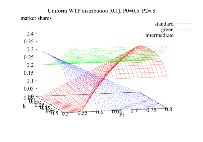
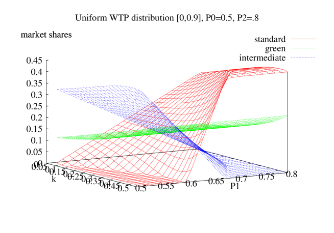
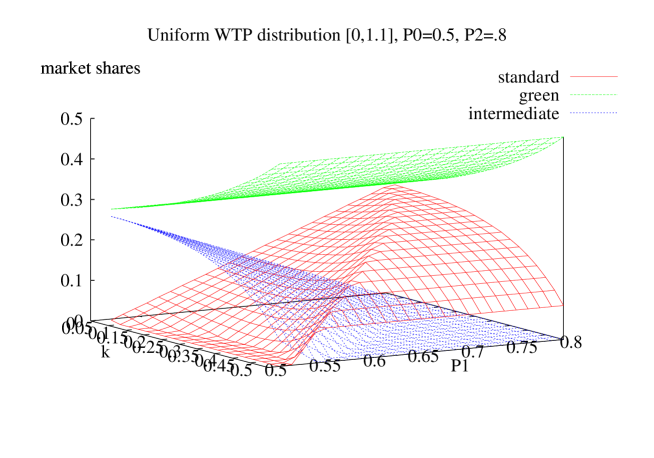
For the above choice of parameters, whether the green product becomes dominant depends essentially from how far $P_{02}$ is from the maximum WTP: in other words what is the potential market share taking only into account the maximum price of the green product. Of course, $u_{2}$ increases with $k$. In fact, $u_{2}$ is independent of $P_{01}$ and $P_{00}$. At equilibrium it always obeys:

$$u_{2}=1-F(P_{02}-ku_{2})$$ (7)

since the ‘green’ product is always chosen when the customer’s WTP is larger than $p_{2}$.

For the uniform WTP distribution this gives:

$$u_{2}=\frac{p_{M}-P_{02}}{p_{M}-p_{m}-k}$$ (8)

where $p_{M}$ and $p_{m}$ are respectively the upper and lower bound of the WTP distribution. This expression is only valid for $k<w$ (check the hysteresis section for the opposite case). In addition, $p_{M}$ should be larger than $P_{02}$ otherwise $u_{2}=0$. It shows that the market share of the green car only depends upon two reduced parameters, $\frac{p_{M}-P_{02}}{p_{M}-p_{m}}$ and $\frac{k}{p_{M}-p_{m}}$.

The competition between the standard and intermediate car, on the other hand, mostly depends upon $P_{01}$: the standard car is favored when $P_{01}$ is close to $P_{02}$, and the intermediate car when $P_{01}$ is close to $P_{00}$.

For the uniform WTP distribution, equations (2) in $u_{2}$, $u_{1}$, and $u_{0}$ are easily solved; the expressions for $u_{2}$, $u_{1}$, and $u_{0}$ depend of the ranking of prices. In the case of $p_{0}\leq p_{1}\leq p_{2}$, they are written in the simple case of a [0,1] WTP distribution:

$$u_{2}=\frac{1-P_{02}}{1-k}$$ (9)

$$u_{1}=\frac{p_{2}-P_{01}}{1-k}$$ (10)

$$u_{0}=\frac{p_{1}-P_{00}}{1-k}$$ (11)

where actual prices $p_{2}$ and $p_{1}$ are obtained from the corresponding values of $u_{i}$. One sees from these equations that markets shares are zero (and the equations have to be re-ordered) whenever $p_{i+1}\leq P_{0i}$. These conditions re-written in terms of initial parameters are:

$$u_{1}=0\quad\mbox{iff}\quad P_{01}\geq\frac{P_{02}-k}{1-k}$$ (12)

$$u_{0}=0\quad\mbox{iff}\quad\mbox{either }P_{00}\geq\frac{P_{01}}{1-k}-\frac{k(P_{02}-k)}{(1-k)^{2}}\mbox{ and }P_{01}<\frac{P_{02}-k}{1-k}$$ (13)

$$\mbox{ or}\quad P_{00}\geq\frac{P_{02}-k}{1-k}\mbox{ and }P_{01}\geq\frac{P_{02}-k}{1-k}$$ (14)

For more general distributions, e.g., the logit distribution, a similar iterative procedure yields market shares and prices, but the equations are transcendental rather than explicitly soluble.

3.3 Hysteresis

Equations such as equation (2) are well-known in physics, e.g., in the Mean Field theory of ferromagnetism [8] and to some extent in economics [9, 10], in the case of increasing returns or social influence. They are known to produce ‘phase’ or ‘regime’ transitions when the number of their solutions goes from one to three as a function of a parameter which is $k/w$ in our case (for the logit distribution $w=4/\beta$).

Figure 8 allows to easily understand the regime transition. It is a graphical solution of equation (2) rewritten as:

$$1-u=F(p-ku).$$ (15)

The curves corresponding to the two sides of the equation are drawn in the plan $(p-ku,1-u)$. The red and black curves correspond to $F(p-ku)$ (respectively, logit and uniform distributions). The blue lines correspond to the left hand side $1-u$ as a function of $p-ku$; it is a straight line, which abscissa is $p$ when $u=0$ and $p-k$ when $u=1$. Two blue lines are drawn corresponding to the two cases of a large $k$, $k_{M}$ and a small $k$, $k_{m}$.

Figure 8: Graphical solution of equation (2) rewritten as $1-u=F(p-ku)$. Abscissa is $x=p-ku$, and ordinate $1-u$. The $F(x)$ curve (cdf), represented in red for the logit distribution of WTP and in black for a uniform distribution, intersects blue lines $1-u$ in one or three points according to the value of $k$ for the particular choice of $p$. $k_{m}\leq 1\leq k_{M}$.

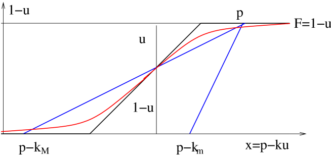
Three solutions may be obtained if the slope of the straight line $1-u$ is lower than the largest slope of the $F$ function. This slope is $k/w$ for the uniform distribution and $4k/\beta$ for the logit distribution. The corresponding conditions for $k$ versus the WTP distribution parameters are thus written:

$$k\geq w$$ (16)

$$k\geq\frac{4}{\beta}$$ (17)

When $k$ is above the threshold, one or three fixed points are then obtained depending upon the value of the maximum price. In the case of three fixed points, the central one is unstable but the two extreme are attractors; which attractor is actually reached depends upon initial conditions: large $u$ values attractor is, e.g., obtained when initially $u(0)=1$ (and small $u$ attractor when $u(0)=0$). The central fixed point separates the two attractor regions.

We considered until now $P_{02}$ as a fixed parameter. Let us now discuss the effect of variations of $P_{02}$, which could be due to technological progress or to strategic moves of the producer of car 2, or to government subsidies etc. The two next figures illustrate the hysteresis cycle when $P_{02}$ is varied, and the transition between the two regimes when both $k$ and $P_{02}$ are varied. They were drawn by superimposing asymptotic simulation results obtained when initial conditions were first $u_{2}(0)=1$ (red curves) and then when $u_{2}(0)=0$ (green curves). In the first case, we thus start without standard or intermediate cars. In the second case, we start with only standard cars. For parameters such that only one attractor exists, only the green curves are visible. But when two are possible, the red curves are visible and correspond to $u_{2}(0)=1$.

Figure 9: A hysteresis cycle obtained for $u_{2}$ when $P_{02}$ is varied. The red curve is $u_{2}$ for $u_{2}(0)=1$ and the green curve when $u_{2}(0)=0$. The increasing returns coefficient $k=2$ is larger than the WTP distribution width $w=4/\beta=1$. The two curves coincide when the price $P_{02}$ is either small or large. They differ in the intermediate price region.

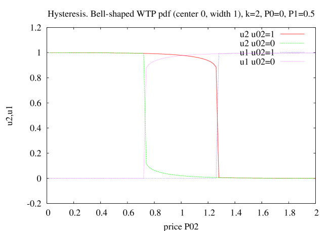
The vertical transitions obtained in the parameter space for the attractor at specific values of $P_{02}$ still correspond to finite time dynamics with a characteristic time of $\lambda^{-1}$.

The middle part of figure 9 can be interpreted as follows. If we have a market that is completely dominated by green cars, the maximum price $P_{02}$ has to rise almost up to 1.3 before the market is taken over by the intermediate or standard car. On the opposite, if the green car does not have a substantial share of the market, the price of the green car has to drop almost to 0.7 before the green car can take over the market.

At the middle of hysteresis loop, $P_{02}$ is one width above the center of the WTP distribution. But since $k=2$, the actual price when $u_{2}=1$ is one width below the center of the distribution. Large values of $k$ imply a strong social influence with respect to price differences: varying $u_{2}$ between 0 and 1 scans a large percentage of the WTP distribution (96 percent). At the transition, $k=\frac{4}{\beta}=1$, this figure is already 63 percent.

Figure 10: Transition between the hysteresis regime and the one attractor regime when $k=\frac{4}{\beta}$. The green sheet is obtained when $u_{2}(0)=1$ and the red sheet when $u_{2}(0)=0$. They differ only in the large $k$ and intermediate $P_{02}$ region.

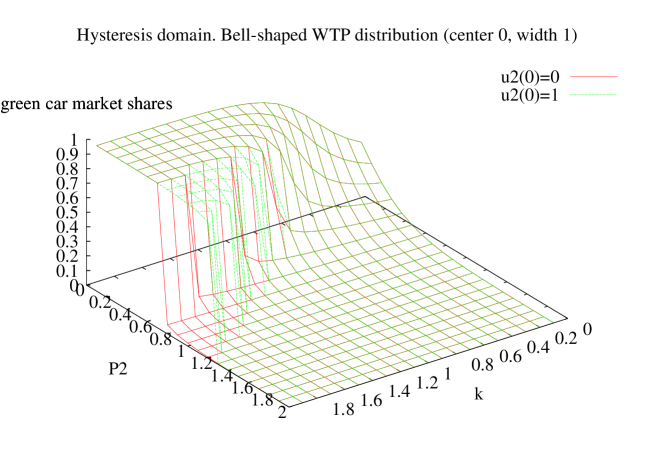
We only discussed until now the dynamics of $u_{2}$ as a function of $k$ and $P_{02}$. Which of the two other products dominates or how they share the market when $u_{2}=0$ depends upon the actual values of $P_{00}$ and $P_{01}$.

Why should we care about hysteresis? After all, our starting assumption was that the intermediate and the green options are introduced after the standard option implying $u_{0}=1,u_{1}=u_{2}=0$ as initial conditions. Since there are several attractors in this regime, the issue of the adoption regime is especially sensitive to the parameter set-up: if we now consider that parameters can be under the influence of decision makers such as producers or government agencies, or exogenous events (e.g., oil prices, technical advances), the hysteresis regime can bring huge consequences for small parameter changes. For instance,

• If price $P_{02}$ is lowered under the action of producers, advertising in the media, or government subsidies, a transition from the $u_{2}\simeq 0$ attractor to the $u_{2}\simeq 1$ attractor can be induced.

• Such an action does not have to be permanent: it might suffice to bring $u_{2}$ above the separatrix, the central fixed point, to bring the system in the basin of attraction of high $u_{2}$.

• Competitors might also have equivalent strategies.

• Sharp transition can be induced in this region through advertising by decision makers, thus changing effective prices for some of the products or the complete WTP distribution.

Multiple attractors are a challenge for scientists, but they are opportunities for decision makers. Of course, parameter changes in the single attractor regime also influence the outcome of the dynamics, but their influence is far less dramatic. Moreover, these effects are reversed as the parameter changes are undone, while the changes under multiple attractors might remain after parameter changes are undone.

4 Conclusions

In this paper, we have illustrated, how one can obtain interpretable but already quite complex dynamics from a simple model on the competition between more or less green technologies assuming that consumers have heterogeneous preferences over these goods. In the first part of the paper we have shown situations in which there was only one attractor for the dynamics. These dynamics show that the prices of the greener alternatives needs to be far enough from the boundary of the willingness to pay distribution to take over the market as well as that the advantages of scale should be large enough to overcome price differences over time. Depending on the precise parameters, several different regimes are possible, differing in the number of equilibrium technologies: 1, 2, or 3. In some situations, green technologies take over only a smaller part of the market, while the standard technology remains dominant. But there are also situations were first the intermediate technology conquers some of the market, and thereafter the most green technology gains some market share and takes most of the market.

Simulations were done with parameters being constant, by definition. One can also infer the results of technological or attitude changes over market shares dynamics. In situations in which there is basically only one attractor, temporary policy measure will not have permanent results because the process will reverse as soon as the policy measure ends.

In the second part of the results, we show that there are also situations in which there are multiple attractors of the dynamics. They typically occur when the width of the willingness to pay distribution is less than the increasing returns coefficient. As long as the market share of the green products is either very small (or very high) the market is stable. However, if some agency is able to raise for some time the fraction of consumers using green cars, or if it could boost for some period the environmental consciousness of enough consumers, the system might jump to the situation in which most people drive in green cars. Such temporary policy measures could then have a stable result even if the measure is only temporary. Of course producers of standard cars could think of measures to get back to the first situation, but these would at least be quite costly for them.

Let us stress that these dynamic properties are generic: they do not depend upon a specific choice of the WTP distribution nor of the increasing return price function. They apply to any S-shape WTP cumulative distribution and any monotonic increasing return function.

Many extensions of the present model are possible, some more application specific, others including coupling with pollution and opinion dynamics, the role of government agencies etc. Some of these extensions might necessitate heavier simulation tools such as multi-agent systems. But anyway, the simple analysis that has been performed here already allows to figure out the influence of the parameters on the observed dynamical regimes and the level of behavioral complexity that can be expected for the heterogeneity of agents and increasing return hypotheses.

Acknowledgments: We thank Jean-Pierre Nadal for illuminating discussions and the participants of the CMAST07 workshop in Leiden (Feb-March 2007). Gérard Weisbuch was also supported by E2C2 NEST 012410 EC grant. Vincent Buskens was supported by the UU-High Potential Program ‘Dynamics of Cooperation, Networks, and Institutions.’

References

- [1] Brian Arthur. Increasing Returns and Path Dependence in the Economy, Univ. of Michigan Press, Ann Arbor, 1994.
- [2] Fran cois Bousquet, Robert Lifran, Mabel Tidball, Sophie Thoyer, and Martine Antona. Agent-based modelling, game theory and natural resource management issues. Journal of Artificial Societies and Social Simulation 4(2), 2001, http://www.soc.surrey.ac.uk/JASSS/4/2/0.html.
- [3] Mirta B. Gordon, Jean-Pierre Nadal, Denis Phan, and Viktoriya Semeshenko. Discrete Choices under Social Influence: Generic Properties, http://halshs.archives-ouvertes.fr/halshs-00135405.
- [4] Mirta B. Gordon, Jean-Pierre Nadal, Denis Phan, and Jean Vannimenus. Seller’s dilemma due to social interactions between customers. Physica A: Statistical Mechanics and its Applications 356(2-4), 15 October 2005, Pages 628-640.
- [5] René Kemp. The Diffusion of Biological Waste-water Treatment Plants in the Dutch Food and Beverage Industry. Environmental and Resource Economics 12, 113 136, 1998.
- [6] Jean-Pierre Nadal, Denis Phan, Mirta B. Gordon, and Jean Vannimenus. Multiple equilibria in a monopoly market with heterogeneous agents and externalities Quantitative Finance 5(6), December 2005, 557-568.
- [7] Gérard Weisbuch. Environment and institutions: a complex dynamical systems approach. Ecological Economics 35(3), December 2000, Pages 381-391
- [8] Charles Kittel and Herbert Kroemer, Thermal Physics 2e, 1980, W.H. Freeman and Co, New York, 1980.
- [9] Föllmer H. (1974) ”Random economies with many interacting agents”, Journal of Mathematical Economics, 1, pp. 51-62.
- [10] Weisbuch, G’erard, Alan P. Kirman and Dorothea K. Herreiner, Market organisation and trading relationships, The Economic Journal, Vol. 110, n 463, 411-436, 2000.