Evolutionary stability in quantum games

Abstract

In evolutionary game theory an Evolutionarily Stable Strategy (ESS) is a refinement of the Nash equilibrium concept that is sometimes also recognized as evolutionary stability. It is a game-theoretic model, well known to mathematical biologists, that was found quite useful in the understanding of evolutionary dynamics of a population. This chapter presents an analysis of evolutionary stability in the emerging field of quantum games.

1 Introduction

Games such as chess, warfare and politics have been played throughout history. Whenever individuals meet who have conflicting desires, and priorities, then games are likely to be played. Analysis and understanding of games has existed for long times but the emergence of game theory as a formal study of games is widely believed to have taken place when Neumann and Morgenstern [1] published their pioneering book “The Theory of Games and Economic Behaviour” in 1944. Game theory [2] is now an established discipline of mathematics that is a vast subject having a rich history and content. Roughly speaking, game theory is the analysis of the actions made by rational players when these actions are strategically interdependent.

The 1970s saw game theory being successfully applied to problems of evolutionary biology and a new branch of game theory, recognized as evolutionary game theory [3, 4, 5], came into existence. The concept of utility from economics was given an interpretation in terms of Darwinian fitness . Originally, evolutionary game theory considered animal conflicts occurring in macro-world. In recent years, research in biology [6] suggested that nature also plays classical games at micro-level. Bacterial infections by viruses are classical game-like situations where nature prefers dominant strategies .

In game theory [1, 2] one finds many examples where multiple Nash equilibria (NE) [7, 8] emerge as solutions of a game. To select one (or possibly more) out of these requires some refinement of the equilibrium concept [9]. A refinement is a rule/criterion that describes the criterion to prefer one (in some cases more than one) equilibrium out of many. Numerous refinements are found in game theory, for example, perfect equilibrium (used for extensive- and normal-form games), sequential equilibrium (a fundamental non-cooperative solution concept for extensive-form games), and correlated equilibrium (used for modelling communication among players).

During recent years quantum game theory [10, 11, 12] has emerged as a new research field within quantum information and computation [13]. A significant portion of research in quantum games deals with the question asking how quantization of a game affects/changes the existence/location of a NE. This question has been addressed in a number of publications [14] in this area and now it seems that it is generally agreed that quantization of a game indeed affects/changes the existence/location of a NE.

In this chapter we argue that, like asking how quantization of a game affects/changes the existence/location of a NE, an equally important question for quantum games is to ask how quantization of a game can affect a refinement of the NE concept. We notice that a particular refinement of the NE, known as an Evolutionarily Stable Strategy (ESS ), is central to evolutionary game theory . While focussing on a this refinement, we motivate those quantum games in which a NE persists in both of its classical and quantum versions while its property of being an ESS survives in either classical or its quantum version, but not in the both. We argue that, the quantum games offering such situations, along with their quantization procedures, can justifiably be said to extend the boundary of investigations in quantum games from existence/location of NE to existence/location of one (or more) of its refinements.

2 Evolutionary game theory and evolutionary stability

The roots of evolutionary game theory [5] can be traced to the puzzle of the approximate equality of the sex ratio in mammals. In 1930 Fisher ( [15, 16]) noticed that if individual fitness is defined in terms of the expected number of grandchildren, then it becomes dependent on how males and females are distributed in a population. Fisher showed that the evolutionary dynamics then leads to the sex ratio becoming fixed at equal numbers of males and females. Although Fisher’s argument can be recast in game-theoretic language but originally it was not presented in those terms. Perhaps it was due to the fact that until that time modern game theory had not yet emerged as a formal study of games.

Modern game theory was used, for the first time, to understand evolution when in 1972 Maynard Smith and G. R. Price introduced the concept of an Evolutionarily Stable Strategy (ESS) [17, 3]. Presently, this concept is widely believed to be the cornerstone of evolutionary game theory [4] and has been found quite useful to explain and understand animal behavior.

Traditionally, game theory had concerned analyzing interactions among hyperrational players and the idea that it can be applied to animals seemed strange at the time. The ESS concept made three important changes in the traditional meaning of the concepts of a) strategy, b) equilibrium, and c) players’ interactions.

a) Strategy : In traditional game theory, players have strategy set from which they choose their strategies. In biology, animals belonging to a species have strategy sets that are genotypic variants that may be mutated, of which individuals inherit one or another variant, which they then play in their strategic interactions. A mixed strategy in game theory means a convex linear combination (with real and normalized coefficients) of pure strategies. Because genotypic variants are taken as pure strategies, the evolutionary game theory interprets a mixed strategy in terms of proportion of the population that is playing that strategy.

b) Equilibrium : An ESS represents an equilibrium and it is a strategy having the property that if a whole population plays it, it cannot be invaded under the influence of natural selection , by a small group of players playing mutant strategies. Because strategies of evolutionary games are genotypes the ESS definition takes the following form: If adapted by a whole population an ESS is a genotype that cannot be invaded by another genotype when it appears in a small fraction of the total population.

c) Player interactions : The ESS concept is about repeated and random pairing of players who play strategies based on their genome and not on the previous history of play. This approach was new to the usual approach of one-shot and repeated games of classical game theory .

Consider a large population [5, 4] in which members are matched repeatedly and randomly in pairs to play a bi-matrix game . The players are anonymous, that is, any pair of players plays the same symmetric bi-matrix game . The symmetry of a bi-matrix game means that for a strategy set $S$ Alice’s payoff when she plays $S_{1}\in S$ and Bob plays $S_{2}\in S$ is the same as Bob’s payoff when he plays $S_{1}$ and Alice plays $S_{2}$. Hence, a player’s payoff is defined by his/her strategy and not by his/her identity and an exchange of strategies by the two players also exchanges their respective payoffs. A symmetric bi-matrix game is represented by an expression $G=(M,M^{T})$ where $M$ is the first player’s payoff matrix and $M^{T}$, being its transpose, is the second players’ payoff matrix . In a symmetric pair-wise contest one can write $P(x,y)$ as being the payoff to a $x$-player against a $y$-player.

To be precise [4, 18, 19] a strategy $x$ is said to be an ESS if:

a) for each mutant strategy $y$ there exists a positive invasion barrier .

b) if the population share of individuals playing the mutant strategy $y$ falls below the invasion barrier, then $x$ earns a higher expected payoff than $y$.

Mathematically speaking [5, 4] $x$ is an ESS when for each strategy $y\neq x$ the inequality

$$P[x,(1-\epsilon)x+\epsilon y]>P[y,(1-\epsilon)x+\epsilon y]$$ (1)

holds for all sufficiently small $\epsilon>0$. In (1) the expression on the left-hand side is payoff to the strategy $x$ when played against the mixed strategy $(1-\epsilon)x+\epsilon y$. This condition for an ESS is shown [17, 3, 5] equivalent to the following requirements:

$$\text{a) }P(x,x) >P(y,x)$$

$$\text{b) If\ }P(x,x) =P(y,x)\text{ then}\ P(x,y)>P(y,y)\text{.}$$ (2)

It turns out [3, 5] that an ESS is a symmetric NE that is stable against small mutations. Condition a) in the definition (2) shows $(x,x)$ is a NE for the bi-matrix game $G=(M,M^{T})$ if $x$ is an ESS . However, the converse is not true. That is, if $(x,x)$ is a NE then $x$ is an ESS only if $x$ satisfies condition b) in definition (2).

Evolutionary game theory defines the concept of fitness [20] of a strategy as follows. Suppose $x$ and $y$ are pure strategies played by a population of players that is engaged in a two-player game. Their fitnesses are

$$W(x)=P(x,x)F_{x}+P(x,y)F_{y};\text{ \ \ }W(y)=P(y,x)F_{x}+P(y,y)F_{y}$$ (3)

where $F_{x}$ and $F_{y}$ are frequencies (the relative proportions) of the pure strategies $x$ and $y$ respectively.

It turned out that an ESS is a refinement on the set of symmetric Nash equilibria [5, 21]. For symmetric bi-matrix games this relationship is described [22] as $\bigtriangleup^{ESS}\subset\bigtriangleup^{PE}\subset\bigtriangleup^{NE}$ where $\bigtriangleup^{PE}\neq\Phi$ and $\bigtriangleup^{NE}$, $\bigtriangleup^{PE}$, $\bigtriangleup^{ESS}$ are the sets of symmetric NE, symmetric proper equilibrium, and ESSs respectively.

The property of an ESS of being robust against small mutations is also referred to as evolutionary stability  [18, 19]. This concept provided a significant part of the motivation for later developments in evolutionary game theory . In evolutionary game theory, the Darwinian natural selection is formulated as an algorithm called replicator dynamics [4, 5] which is a mathematical statement saying that in a population the proportion of players playing better strategies increases with time. Mathematically, ESSs come out as the rest points of replicator dynamics [4, 5].

Evolutionary stability was found to be a useful concept because it says something about the dynamic properties of a system without being committed to a particular dynamic model. Sometimes, it is also described as a model of rationality which is physically grounded in natural selection .

2.1 Population setting of evolutionary game theory

Evolutionary game theory introduces so-called the population setting [5, 4] that is also known as population-statistical setting . This setting assumes a) an infinite population of players who are engaged in random pair-wise contests b) each player being programmed to play only one strategy and c) an evolutionary pressure ensuring that better-performing strategies have better chances of survival at the expense of other competing strategies. Because of b) one can refer to better-performing players as better-performing strategies.

The population setting of evolutionary game theory is not alien to the concept of the NE, although it may give such an impression. In fact, John Nash himself had this setting in his mind when he introduced this concept in game theory. In his unpublished Ph.D. thesis [23, 4] he wrote ‘it is unnecessary to assume that the participants have…the ability to go through any complex reasoning process. But the participants are supposed to accumulate empirical information on the various pure strategies at their disposal…We assume that there is a population…of participants…and that there is a stable average frequency with which a pure strategy is employed by the “average member” of the appropriate population’.

That is, Nash had suggested a population interpretation of the NE concept in which players are randomly drawn from large populations. Nash assumed that these players were not aware of the total structure of the game and did not have either the ability nor inclination to go through any complex reasoning process.

3 Quantum games

This chapter considers evolutionary stability in quantum games that are played in the two quantization schemes: Eisert, Wilkens, Lewenstein (EWL) scheme [11, 12] for playing quantum Prisoners’ Dilemma (PD) and Marinatto and Weber (MW) scheme [24] for playing quantum Battle of Sexes (BoS) game.

EWL quantization scheme appeared soon after Meyer’s publication [10] of the PQ penny-flip – a quantum game that generated significant interest and is widely believed to have led to the creation of the new research field of quantum games . MW scheme derives from EWL scheme but it gives a different meaning to the term ‘strategy’ [25, 26].

EWL quantum PD assigns two basis vectors $\left|C\right\rangle$ and $\left|D\right\rangle$ in the Hilbert space of a qubit . States of the two qubits belong to two-dimensional Hilbert spaces $H_{A}$ and $H_{B}$, respectively. The state of the game is defied as being a vector residing in the tensor-product space $H_{A}\otimes H_{B}$, spanned by the basis $\left|CC\right\rangle,\left|CD\right\rangle,\left|DC\right\rangle$ and $\left|DD\right\rangle$. Game’s initial state is $\left|\psi_{ini}\right\rangle=\hat{J}\left|CC\right\rangle$ where $\hat{J}$ is a unitary operator known to both the players. Alice’s and Bob’s strategies are unitary operations $\hat{U}_{A}$ and $\hat{U}_{B}$, respectively, chosen from a strategic space Ş. After players’ actions the state of the game changes to $\hat{U}_{A}\otimes\hat{U}_{B}\hat{J}\left|CC\right\rangle$. Finally, the state is measured and it consists of applying reverse unitary operator $\hat{J}^{\dagger}$ followed by a pair of Stern-Gerlach type detectors . Before detection the final state of the game is $\left|\psi_{fin}\right\rangle=\hat{J}^{\dagger}\hat{U}_{A}\otimes\hat{U}_{B}\hat{J}\left|CC\right\rangle$. Players’ expected payoffs are the projections of the state $\left|\psi_{fin}\right\rangle$ onto the basis vectors of tensor-product space $H_{A}\otimes H_{B}$, weighed by the constants appearing in the following game matrix (4).

$$\begin{array}[c]{c}\text{Alice}\end{array}\begin{array}[c]{c}C\\ D\end{array}\overset{\overset{\begin{array}[c]{c}\text{Bob}\end{array}}{\begin{array}[c]{cc}C&D\end{array}}}{\left(\begin{array}[c]{cc}(r,r)&(s,t)\\ (t,s)&(u,u)\end{array}\right)}$$ (4)

where $C$ and $D$ are the classical strategies of Cooperation and Defection, respectively. The first and the second entry in small braces correspond to Alice’s and Bob’s (classical, pure strategy) payoffs, respectively. When $s<u<r<t$ the matrix (4) represents PD. In EWL quantum PD Alice’s payoff, for example, reads

$$P_{A}=r\left|\left\langle CC\mid\psi_{fin}\right\rangle\right|^{2}+s\left|\left\langle CD\mid\psi_{fin}\right\rangle\right|^{2}+t\left|\left\langle DC\mid\psi_{fin}\right\rangle\right|^{2}+u\left|\left\langle DD\mid\psi_{fin}\right\rangle\right|^{2}\text{.}$$ (5)

With reference to the matrix (4) Bob’s payoff is, then, obtained by the transformation $s\rightleftarrows t$ in Eq. (5). Eisert and Wilkens [12] used following matrix representations of unitary operators of their one- and two-parameter strategies, respectively:

$$U(\theta) =\left(\begin{array}[c]{cc}\cos(\theta/2)&\sin(\theta/2)\\ \text{-}\sin(\theta/2)&\cos(\theta/2)\end{array}\right)$$ (8)

$$U(\theta,\phi) =\left(\begin{tabular}[c]{ll}e${}^{i\phi}\cos(\theta/2)$&$\sin(\theta/2)$\\ $\text{-}\sin(\theta/2)$&e${}^{-i\phi}\cos(\theta/2)$\end{tabular}\right)$$ (11)

where

$$0\leq\theta\leq\pi\text{ and }0\leq\phi\leq\pi/2\text{.}$$ (12)

To ensure that the classical game is faithfully represented in its quantum version, EWL imposed an additional conditions on $\hat{J}$:

$$\left[\hat{J},\hat{D}\otimes\hat{D}\right]=0,\left[\hat{J},\hat{D}\otimes\hat{C}\right]=0,\left[\hat{J},\hat{C}\otimes\hat{D}\right]=0$$ (13)

with $\hat{C}$ and $\hat{D}$ being the operators corresponding to the classical strategies $C$ and $D$, respectively. A unitary operator satisfying the condition (13) is

$$\hat{J}=\exp\left\{i\gamma\hat{D}\otimes\hat{D}/2\right\}$$ (14)

where $\gamma\in\left[0,\pi/2\right]$ and $\hat{J}$ represents a measure of the game’s entanglement . At $\gamma=0$ the game can be interpreted as a mixed-strategy classical game. For a maximally entangled game $\gamma=\pi/2$ the classical NE of $\hat{D}\otimes\hat{D}$ is replaced by a different unique equilibrium $\hat{Q}\otimes\hat{Q}$ where $\hat{Q}\sim\hat{U}(0,\pi/2).$ This new equilibrium is found also to be Pareto optimal  [2], that is, a player cannot increase his/her payoff by deviating from this pair of strategies without reducing the other player’s payoff. Classically $(C,C)$ is Pareto optimal, but is not an equilibrium [2], thus resulting in the ‘dilemma’ in the game. It is argued [27, 28] that in its quantum version the dilemma disappears from the game and quantum strategies give a superior performance if entanglement is present.

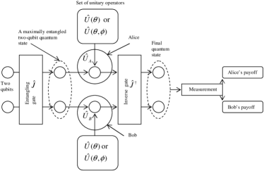
Figure 1: EWL scheme to play a quantum game.

MW quantization scheme [24, 25, 26] for BoS identifies a state in $2\otimes 2$ dimensional Hilbert space as a strategy. At the start of the game the players are supplied with this strategy and the players manipulate the strategy in the next phase by playing their tactics. The state is finally measured and payoffs are rewarded depending on the results of the measurement. A player can do actions within a two-dimensional subspace. Tactics are therefore local actions on a player’s qubit. The final measurement, made independently on each qubit , takes into consideration the local nature of players’ manipulations. This is done by selecting a measurement basis that respects the division of Hilbert space into two equal parts.

Essentially MW scheme differs from EWL scheme [11, 12] in the absence of reverse gate $J^{\dagger}$. Finally, the quantum state is measured and it is found that the classical game remains a subset of the quantum game if the players’ tactics are limited to a convex linear combination, with real coefficients, of applying the identity $\hat{I}$ and the Pauli spin-flip operator $\hat{\sigma}_{x}$. Classical game results when the players are forwarded an initial strategy $\left|\psi_{in}\right\rangle=\left|00\right\rangle$.

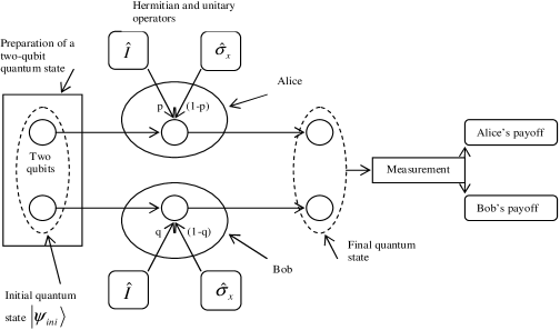
Figure 2: MW scheme to play a quantum game.

Let $\rho_{in}$ be the initial strategy the players Alice and Bob receive at the start of the game. Assume Alice acts with identity $\hat{I}$ on $\rho_{in}$ with probability $p$ and with $\hat{\sigma}_{x}$ with probability $(1-p)$. Similarly, Bob act with identity $\hat{I}$ with probability $q$ and with $\hat{\sigma}_{x}$ with probability $(1-q)$. After players’ actions the state changes to

$$\rho_{fin} =pq\hat{I}_{A}\otimes\hat{I}_{B}\rho_{in}\hat{I}_{A}^{\dagger}\otimes\hat{I}_{B}^{\dagger}+p(1-q)\hat{I}_{A}\otimes\hat{\sigma}_{xB}\rho_{in}\hat{I}_{A}^{\dagger}\otimes\hat{\sigma}_{xB}^{\dagger}+$$

$$q(1-p)\hat{\sigma}_{xA}\otimes\hat{I}_{B}\rho_{in}\hat{\sigma}_{xA}^{\dagger}\otimes\hat{I}_{B}^{\dagger}+$$

$$(1-p)(1-q)\hat{\sigma}_{xA}\otimes\hat{\sigma}_{xB}\rho_{in}\hat{\sigma}_{xA}^{\dagger}\otimes\hat{\sigma}_{xB}^{\dagger}\text{.}$$ (15)

When the game is given by the bi-matrix:

$$\begin{array}[c]{c}\text{Alice}\end{array}\begin{array}[c]{c}S_{1}\\ S_{2}\end{array}\overset{\overset{\begin{array}[c]{c}\text{Bob}\end{array}}{\begin{array}[c]{cc}S_{1}&S_{2}\end{array}}}{\left(\begin{array}[c]{cc}(\alpha_{A},\alpha_{B})&(\beta_{A},\beta_{B})\\ (\gamma_{A},\gamma_{B})&(\delta_{A},\delta_{B})\end{array}\right)}$$ (16)

the payoff operators are:

$$(P_{A})_{oper} =\alpha_{A}\left|00\right\rangle\left\langle 00\right|+\beta_{A}\left|01\right\rangle\left\langle 01\right|+\gamma_{A}\left|10\right\rangle\left\langle 10\right|+\delta_{A}\left|11\right\rangle\left\langle 11\right|$$

$$(P_{B})_{oper} =\alpha_{B}\left|00\right\rangle\left\langle 00\right|+\beta_{B}\left|01\right\rangle\left\langle 01\right|+\gamma_{B}\left|10\right\rangle\left\langle 10\right|+\delta_{B}\left|11\right\rangle\left\langle 11\right|\text{.}$$ (17)

and payoff functions are then obtained as mean values of these operators:

$$P_{A,B}=Tr\left\{(P_{A,B})_{oper}\rho_{fin}\right\}\text{.}$$ (18)

It is to be pointed out that in EWL set-up a quantum game corresponds when the entanglement parameter $\gamma$ of the initial quantum state is different from zero. When $\gamma$ is non-zero the players have strategies available to them that result in the classical game. The general idea is to allow a range of values to the parameter $\gamma$ and then to find how it leads to a different, i.e. non-classical, equilibrium in the game.

In MW scheme [24, 25, 26] an initial strategy is forwarded to two players who then apply their tactics on it and the classical game corresponds to the initial state $\left|00\right\rangle$. Assume now that the players receive pure two-qubit states, different from $\left|00\right\rangle$, and the measurement remains the same. A quantum form of the game then corresponds if initial states different from the product state $\left|00\right\rangle$ are used. This translates finding quantum form of a matrix game to finding appropriate initial state(s). This is justified because the only restriction [26] on a quantum form of a game being that the corresponding classical game must be reproducible as its special case. As the product initial state $\left|00\right\rangle$ always results in the classical game, this approach remains within the mentioned restriction.

In EWL scheme one looks for new equilibria in games in relation to the parameter $\gamma$. In the above approach, however, one finds equilibria in relation to different initial states. In this chapter, we will restrict ourselves to pure states only.

4 Evolutionary stability in quantum games

The concept of a NE was addressed in the earliest research publications in quantum games [11, 12]. Analysis of this solution concept from non-cooperative game theory generated significant interest in the new research field. These publications do not explicitly refer to the population interpretation of the NE concept. In fact, this possibility of this interpretation was behind the development of the ESS concept in evolutionary game theory. And when this interpretation is brought within the domain of quantum games it becomes natural to consider ESSs in this domain.

One may ask how and where the population setting may be relevant to quantum games . How can a setting, originally developed to model the population biology problems, be relevant and useful to quantum games ? One can often sharpen this argument given the fact that, to date, almost all of the experimental realizations of quantum games are artificially constructed in laboratories using quantum computational circuits [13].

Several replies can be made to this question, for example, that this setting was behind the development of the NE concept that was addressed in the earliest constructions of quantum games attracting significant attention. One also finds that evolutionary stability has very rich literature in game theory, mathematical biology and in evolutionary economics [29, 30]. In quantum games the NE has been discussed in relation to quantum entanglement [13] and the possibility that the same can be done with evolutionary stability clearly opens a new interesting role for this quantum phenomenon. It is conjectured that the possibility of this extended role for entanglement may perhaps be helpful to better understand entanglement itself.

Evolutionary stability presents a game-theoretic model to understand evolutionary dynamics. Recent developments in quantum games motivate to ask how this game-theoretic solution concept adapts/shapes/changes itself when players are given access to quantum strategies . This questions is clearly related to a bigger question: Can quantum mechanics have a role in directing, or possibly dictating, the dynamics of evolution? We believe that for an analysis along this direction the evolutionary stability offers an interesting situation because, firstly, it is a simple and a beautiful concept and, secondly, it is supported by extensive literature [18, 4].

To discuss evolutionary stability in quantum games may appear as if a concept originally developed for population biology problems is arbitrarily being placed within the domain of quantum games. One can reply to this by noticing that population biology is not the only relevant domain for the concept of evolutionary stability . This concept can also be interpreted using infinitely repeated two-player games and without referring to a population of players. Secondly, as the Nash’s thesis [23, 4] showed it, it is not the population biology alone that motivates a population setting for game theory – responsible for the concept of evolutionary stability . Surprisingly, the concept of NE also does the same, although it may not be recognized generally.

The usual approach in game theory consists of analyzing games among hyper-rational players who are always found both ready and engaged in their selfish interests to optimize their payoffs or utilities. Evolutionary stability has roots in the efforts to get rid of this usual approach that game theory had followed. The lesson it teaches is that playing games can be disassociated from players’ capacity to make rational decisions. This disassociation seems equally valid in those possible situations where nature plays quantum games . It is because associating rationality to quantum-interacting entities is of even a more remote possibility than it is the case when this association is made to bacteria and viruses, whose behavior evolutionary game theory explains.

In the following we will try to address the following questions: How ESSs are affected when a classical game, played by a population, changes itself to a quantum form? How pure and mixed ESSs are distinguished from one another when such a change in the form of a game takes place? Can quantum games provide a route that can relate evolutionary dynamics, for example, to quantum entanglement ? Considering a population of players in which a classical strategy has established itself as an ESS , we would like to ask: a) What happens when ‘mutants’ of ESS theory come up with quantum strategies and try to invade the classical ESS? b) What happens if such an invasion is successful and a new ESS is established – an ESS that is quantum in nature? c) Suppose afterwards another small group of mutants appears which is equipped with some other quantum strategy . Will it successfully invade the quantum ESS?

4.1 Evolutionary stability in EWL scheme

EWL used the matrix (4) with $r=3,s=0,t=5,$ and $u=1$ in their proposal for quantum PD. Assume a population setting where in each pair-wise encounter the players play PD with the same matrix and each contest is symmetric. Which strategies will then be likely to be stable? Straightforward analysis [20] shows that $D$ will be the pure classical strategy prevalent in the population and hence the classical ESS. We consider following three cases:

Case (a) A small group of mutants appear equipped with one-parameter quantum strategy $\hat{U}(\theta)$ when $D$ exists as a classical ESS

Case (b) Mutants are equipped with two-parameter quantum strategy $\hat{U}(\theta,\phi)$ against the classical ESS

Case (c) Mutants have successfully invaded and a two-parameter quantum strategy $\hat{Q}\sim\hat{U}(0,\pi/2)$ has established itself as a new quantum ESS. Again another small group of mutants appear, using some other two-parameter quantum strategy, and tries to invade the quantum ESS, which is $\hat{Q}$.

Case (a):

Because players are anonymous one can represent $P(\hat{U}(\theta),D)$ as the payoff to $\hat{U}(\theta)$-player against the $D$-player. Here $\hat{U}(\theta)$ is the Eisert and Wilkens’ one-parameter quantum strategy set (8). Players’ payoffs read $P(\hat{U}(\theta),D)=\sin^{2}(\theta/2)$; $P(\hat{U}(\theta),\hat{U}(\theta))=2\cos^{2}(\theta/2)+5\cos^{2}(\theta/2)\sin^{2}(\theta/2)+1$; $P(D,\hat{U}(\theta))=5\cos^{2}(\theta/2)+\sin^{2}(\theta/2)$; and $P(D,D)=1$. Now $P(D,D)>P(\hat{U}(\theta),D)$ for all $\theta\in[0,\pi)$. Hence the first condition for an ESS holds and $D\sim\hat{U}(\pi)$ is an ESS. The case $\theta=\pi$ corresponds to one-parameter mutant strategy coinciding with the ESS, which is ruled out. If $D\sim\hat{U}(\pi)$ is played by almost all the members of the population – which corresponds to high frequency $F_{D}$ for $D$ – we then have $W(D)>W(\theta)$ for all $\theta\in[0,\pi)$ using the definition (3). The fitness of a one-parameter quantum strategy, therefore, cannot exceed the fitness of a classical ESS. And a one-parameter quantum strategy cannot invade a classical ESS.

Case (b):

Let $\hat{U}(\theta,\phi)$ be a two-parameter strategy from the set (11). The expected payoffs read $P(D,D)=1$; $P(D,\hat{U}(\theta,\phi))=5\cos^{2}(\phi)\cos^{2}(\theta/2)+\sin^{2}(\theta/2)$; $P(\hat{U}(\theta,\phi),D)=5\sin^{2}(\phi)\cos^{2}(\theta/2)+\sin^{2}(\theta/2)$; and

$$P(\hat{U}(\theta,\phi),\hat{U}(\theta,\phi)) =3\left|\cos(2\phi)\cos^{2}(\theta/2)\right|^{2}$$

$$+5\cos^{2}(\theta/2)\sin^{2}(\theta/2)\left|\sin(\phi)-\cos(\phi)\right|^{2}$$

$$+\left|\sin(2\phi)\cos^{2}(\theta/2)+\sin^{2}(\theta/2)\right|^{2}\text{.}$$ (19)

Here $P(D,D)>P(\hat{U}(\theta,\phi),D)$ if $\phi<\arcsin(1/\sqrt{5})$ and if $P(D,D)=P(\hat{U}(\theta,\phi),D)$ then $P(D,\hat{U}(\theta,\phi))>P(\hat{U}(\theta,\phi),\hat{U}(\theta,\phi))$. Therefore, $D$ is an ESS if $\phi<\arcsin(1/\sqrt{5})$ otherwise the strategy $\hat{U}(\theta,\phi)$ will be in position to invade $D$. Alternatively, if most of the members of the population play $D\sim\hat{U}(\pi,0)$ – which means a high frequency $F_{D}$ for $D$ – then the fitness $W(D)$ will remain greater than the fitness $W[\hat{U}(\theta,\phi)]$ if $\phi<\arcsin(1/\sqrt{5})$. For $\phi>\arcsin(1/\sqrt{5})$ the strategy $\hat{U}(\theta,\phi)$ can invade the strategy $D$, which is the classical ESS.

In this analysis mutants are able to invade $D$ when $\phi>\arcsin(1/\sqrt{5})$ and the invasion may seem not so unusual given the fact that they exploit richer strategies. But it leads to the third case i.e. when ‘quantum mutants ’ have successfully invaded and a two-parameter strategy $\hat{U}$ has established itself. Can now some new mutants coming up with $\hat{Q}\sim\hat{U}(0,\pi/2)$ and invade the ‘quantum ESS’?

Case (c):

EWL [11, 12] showed that in their quantum PD the quantum strategy $\hat{Q}$, played by both the players, is the unique NE. How mutants playing $\hat{Q}$ come up against $\hat{U}(\theta,\phi)$ which already exists as an ESS? To find it the following payoffs are obtained. $P(\hat{Q},\hat{Q})=3$; $P(\hat{U}(\theta,\phi),\hat{Q})=[3-2\cos^{2}(\phi)]\cos^{2}(\theta/2)$; and $P(\hat{Q},\hat{U}(\theta,\phi))=[3-2\cos^{2}(\phi)]\cos^{2}(\theta/2)+5\sin^{2}(\theta/2)$. Now the inequality $P(\hat{Q},\hat{Q})>P(\hat{U}(\theta,\phi),\hat{Q})$ holds for all $\theta\in[0,\pi]$ and $\phi\in[0,\pi/2]$ except when $\theta=0$ and $\phi=\pi/2$, which is the case when the mutant strategy $\hat{U}(\theta,\phi)$ is the same as $\hat{Q}$. This case is obviously ruled out. The first condition for $\hat{Q}$ to be an ESS, therefore, holds. The condition $P(\hat{Q},\hat{Q})=P(\hat{U}(\theta,\phi),\hat{Q})$ implies $\theta=0$ and $\phi=\pi/2$. Again we have the situation of mutant strategy same as $\hat{Q}$ and the case is neglected. If $\hat{Q}$ is played by most of the players, meaning high frequency $F_{\hat{Q}}$ for $\hat{Q}$, then $W(\hat{Q})>W[\hat{U}(\theta,\phi)]$ for all $\theta\in(0,\pi]$ and $\phi\in[0,\pi/2)$. A two-parameter quantum strategy $\hat{U}(\theta,\phi)$, therefore, cannot invade the quantum ESS (i.e. the strategy $\hat{Q}\sim\hat{U}(0,\pi/2)$). Mutants’ access to richer strategies, as it happens in the case (B), does not continue to be an advantage as most of the population also have access to it. Hence $\hat{Q}$ comes out as the unique NE and ESS of the game.

4.1.1 Evolutionary stability and entanglement

Above analysis motivates to obtain a direct relationship between a measure of entanglement and the mathematical concept of evolutionary stability for two-player games. The following example shows this relationship. Consider the two-player game given by the matrix (20):

$$\begin{array}[c]{c}\text{Alice}\end{array}\begin{array}[c]{c}S_{1}\\ S_{2}\end{array}\overset{\overset{\begin{array}[c]{c}\text{Bob}\end{array}}{\begin{array}[c]{cc}S_{1}&S_{2}\end{array}}}{\left(\begin{array}[c]{cc}(r,r)&(s,t)\\ (t,s)&(u,u)\end{array}\right)}$$ (20)

and suppose Alice and Bob play the strategy $S_{1}$ with probabilities $p$ and $q$, respectively. The strategy $S_{2}$ is then played with probabilities $(1-p)$ and $(1-q)$ by Alice and Bob, respectively. We denote Alice’s payoff by $P_{A}(p,q)$ when she plays $p$ and Bob plays $q$. That is, Alice’s and Bob’s strategies are now identified by the numbers $p,q\in[0,1]$, without referring to $S_{1}$ and $S_{2}$. For the matrix (20) Alice’s payoff $P_{A}(p,q)$, for example, reads

$$P_{A}(p,q)=rpq+sp(1-q)+t(1-p)q+u(1-p)(1-q)\text{.}$$ (21)

Similarly, Bob’s payoff $P_{B}(p,q)$ can be written. In this symmetric game we have $P_{A}(p,q)=P_{B}(q,p)$ and, without using subscripts, $P(p,q)$, for example, describes the payoff to $p$-player against $q$-player. In this game the inequality

$$P(p^{\ast},p^{\ast})-P(p,p^{\ast})\geqslant 0$$ (22)

says that the strategy $p^{\ast}$, played by both the players, is a NE. We consider the case when

$$s=t,\text{ \ \ }r=u\text{ and \ \ }(r-t)>0$$ (23)

in the matrix (20). In this case the inequality (22) along with the definition (21) gives

$$P(p^{\ast},p^{\ast})-P(p,p^{\ast})=(p^{\ast}-p)(r-t)(2p^{\ast}-1)$$ (24)

and the strategy $p^{\ast}=1/2$ comes out as a mixed NE. From the ESS definition (2) we get $P(1/2,1/2)-P(p,1/2)=0$ and the part a) of the definition does not apply. Part b) of the definition (2), then, gives

$$P(1/2,p)-P(p,p)=(r-t)\left\{2p(1-p)-1/2\right\}$$ (25)

which can not be strictly greater than zero given $(r-t)>0$. For example, at $p=0$ it becomes a negative quantity. Therefore, for the matrix game defined by (20) and (23) the strategy $p^{\ast}=1/2$ is a symmetric NE, but it is not evolutionarily stable. Also, at this equilibrium both players get $(r+t)/2$ as their payoffs.

Now consider the same game, defined by (20) and (23), when it is played by the set-up proposed by EWL. We set $s_{A}\equiv(\theta_{A},\phi_{A})$ and $s_{B}\equiv(\theta_{B},\phi_{B})$ to denote Alice’s and Bob’s strategies, respectively. Because the quantum game is symmetric i.e. $P_{A}(s_{A},s_{B})=P_{B}(s_{B},s_{A})$ we can write, as before, $P(s_{A},s_{B})$ for the payoff to $s_{A}$-player against $s_{B}$-player. For the quantum form of the game defined by (20,23) one finds

$$P(s_{A},s_{B})=(1/2)(r-t)\left\{1+\cos\theta_{A}\cos\theta_{B}+\sin\theta_{A}\sin\theta_{B}\sin\gamma\sin(\phi_{A}+\phi_{B})\right\}+t\text{.}$$ (26)

The definition of a NE gives $P(s^{\ast},s^{\ast})-P(s,s^{\ast})\geqslant 0$ where $s=(\theta,\phi)$ and $s^{\ast}=(\theta^{\ast},\phi^{\ast})$. This definition can be written as

$$\left\{\partial_{\theta}P\mid_{\theta^{\ast},\phi^{\ast}}(\theta^{\ast}-\theta)+\partial_{\phi}P\mid_{\theta^{\ast},\phi^{\ast}}(\phi^{\ast}-\phi)\right\}\geq 0\text{.}$$ (27)

We search for a quantum strategy $s^{\ast}=(\theta^{\ast},\phi^{\ast})$ for which both $\partial_{\theta}P\mid_{\theta^{\ast},\phi^{\ast}}$ and $\partial_{\phi}P\mid_{\theta^{\ast},\phi^{\ast}}$ vanish at $\gamma=0$ and which, at some other value of $\gamma$, is not zero. For the payoffs (26) the strategy $s^{\ast}=(\pi/2,\pi/4)$ satisfies these conditions. For this strategy Eq. (26) gives

$$P(s^{\ast},s^{\ast})-P(s,s^{\ast})=(1/2)(r-t)\sin\gamma\left\{1-\sin(\phi+\pi/4)\sin\theta\right\}\text{.}$$ (28)

At $\gamma=0$ the strategy $s^{\ast}=(\pi/2,\pi/4)$, when played by both the players, is a NE and it rewards the players same as does the strategy $p^{\ast}=1/2$ in the classical version of the game i.e. $(r+t)/2$. Also, then we have $P(s^{\ast},s^{\ast})-P(s,s^{\ast})=0$ from Eq. (28) and the ESS’s second condition in (2) applies. Use Eq. (26) to evaluate

$$P(s^{\ast},s)-P(s,s) =-(r-t)\cos^{2}(\theta)+$$

$$(1/2)(r-t)\sin\gamma\sin\theta\left\{\sin(\phi+\pi/4)-\sin\theta\sin(2\phi)\right\}$$ (29)

which at $\gamma=0$ reduces to $P(s^{\ast},s)-P(s,s)=-(r-t)\cos^{2}(\theta)$, that can assume negative values. The game’s definition (23) and the ESS’s second condition in (2) show that the strategy $s^{\ast}=(\pi/2,\pi/4)$ is not evolutionarily stable at $\gamma=0$.

Now consider the case when $\gamma\neq 0$ in order to know about the evolutionary stability of the same quantum strategy. From (12) we have both $\sin\theta,\sin(\phi+\pi/4)\in[0,1]$ and Eq. (28) indicates that $s^{\ast}=(\pi/2,\pi/4)$ remains a NE for all $\gamma\in[0,\pi/2]$. The product $\sin(\phi+\pi/4)\sin\theta$ attains a value of $1$ only at $s^{\ast}=(\pi/2,\pi/4)$ and remains less than $1$ otherwise. Eq. (28) shows that for $\gamma\neq 0$ the strategy $s^{\ast}=(\pi/2,\pi/4)$ becomes a strict NE for which the ESS’s first condition in (2) applies. Therefore, for the game defined in (23) the strategy $s^{\ast}=(\pi/2,\pi/4)$ is evolutionarily stable for a non-zero measure of entanglement $\gamma$. That is, entanglement gives evolutionary stability to a symmetric NE by making it a strict NE, that is, it is achieved by using in (2) the ESS’s first condition only. Perhaps, a more interesting example would be the case when entanglement gives evolutionary stability via the ESS’s second condition. In that case, entanglement will make $P(s^{\ast},s)$ strictly greater than $P(s,s)$ when $P(s^{\ast},s^{\ast})$ and $P(s,s^{\ast})$ are equal.

It is to be pointed out here that in literature there exists an approach [31] which characterizes ESSs in terms of extremal states of a function known as evolutionary entropy that is defined by

$$E=-\underset{i}{\sum}\mu_{i}\log\mu_{i}$$ (30)

where $\mu_{i}$ represents the relative contribution of the $i$-th strategy to the total payoff. A possible extension of the present approach may be the case when quantum entanglement decides extremal states of evolutionary entropy. Extension along similar lines can be proposed for another quantity called relative negentropy [18] that is optimized during the course of evolution.

4.2 Evolutionary stability in MW quantization scheme

Another interesting route that allows to consider evolutionary stability in relation to quantization of a game is provided by MW scheme [24]. In this scheme a transition between classical and quantum game is achieved by the initial state: classical payoffs are obtained when the initial state is a product state $\left|\psi_{in}\right\rangle=\left|00\right\rangle$. In this scheme one can consider evolutionary stability in a quantum game by asking whether it possible that a particular symmetric NE switches-over between being an ESS and not being an ESS when the initial state (initial strategy) changes from being $\left|\psi_{in}\right\rangle=\left|00\right\rangle$ to another state. MW scheme offers the possibility to make transition from classical to quantum version of a game by using different initial states and it appears to be a more suitable quantization scheme to analyze evolutionary stability in quantum games. It is because:

a) In a symmetric bi-matrix game , played in a population setting, players have access to two pure strategies and a mixed strategy is interpreted as a convex linear combination of pure strategies. Similar is the case with the players’ strategies in MW scheme where a mixed strategy consists of a convex linear combination of the players’ actions with two unitary operators .

b) Fitness of a pure strategy can be given a straightforward extension in MW scheme . It corresponds to a situation when, for example, in the quantum game, a player uses only one unitary operator out of the two.

c) Theory of ESSs, in the classical domain, deals with anonymous players possessing discrete number of pure strategies. EWL scheme involves a continuum of pure quantum strategies . The ESS concept is known to encounter problems [32] when players possess a continuum of pure strategies.

4.2.1 $2\times 2$ asymmetric games

An ESS is defined as a strict NE [5] for an asymmetric bi-matrix game, i.e. the game $G=(M,N)$ for which $N\neq M^{T}$. That is, a strategy pair $(\overset{\star}{x},\overset{\star}{y})\in S$ is an ESS of the game $G$ if $P_{A}(\overset{\star}{x},\overset{\star}{y})>P_{A}(x,\overset{\star}{y})$ and $P_{B}(\overset{\star}{x},\overset{\star}{y})>P_{B}(\overset{\star}{x},y)$ for all $x\neq\overset{\star}{x}$ and $y\neq\overset{\star}{y}$. For example, the BoS:

$$\left(\begin{array}[c]{cc}(\alpha,\beta)&(\gamma,\gamma)\\ (\gamma,\gamma)&(\beta,\alpha)\end{array}\right)$$ (31)

where $\alpha>\beta>\gamma$ is a asymmetric game with three classical NE [24] given as 1) $\overset{\star}{p_{1}}=\overset{\star}{q_{1}}=0$ 2) $\overset{\star}{p_{2}}=\overset{\star}{q_{2}}=1$ and 3) $\overset{\star}{p_{3}}=\frac{\alpha-\gamma}{\alpha+\beta-2\gamma},\overset{\star}{q_{3}}=\frac{\beta-\gamma}{\alpha+\beta-2\gamma}$. Here the NE 1) and 2) are also ESS’s but 3) is not because of not being a strict NE. When the asymmetric game (31) is played with the initial state $\left|\psi_{in}\right\rangle=a\left|S_{1}S_{1}\right\rangle+b\left|S_{2}S_{2}\right\rangle$, where $S_{1}$ and $S_{2}$ are players’ pure classical strategies, the following three NE [24] emerge 1) $\overset{\star}{p_{1}}=\overset{\star}{q_{1}}=1$ 2) $\overset{\star}{p_{2}}=\overset{\star}{q_{2}}=0$ and 3) $\overset{\star}{p_{3}}=\frac{(\alpha-\gamma)\left|a\right|^{2}+(\beta-\gamma)\left|b\right|^{2}}{\alpha+\beta-2\gamma},\overset{\star}{q_{3}}=\frac{(\alpha-\gamma)\left|b\right|^{2}+(\beta-\gamma)\left|a\right|^{2}}{\alpha+\beta-2\gamma}$. It turns out that, similar to the classical case, the quantum NE $1$) and $2$) are ESSs while $3$) is not. Now, play thsi game with a different initial state:

$$\left|\psi_{in}\right\rangle=a\left|S_{1}S_{2}\right\rangle+b\left|S_{2}S_{1}\right\rangle$$ (32)

for which players’ payoffs are:

$$P_{A}(p,q) =p\left\{-q(\alpha+\beta-2\gamma)+\alpha\left|a\right|^{2}+\beta\left|b\right|^{2}-\gamma\right\}+$$

$$q\left\{\alpha\left|b\right|^{2}+\beta\left|a\right|^{2}-\gamma\right\}+\gamma$$

$$P_{B}(p,q) =q\left\{-p(\alpha+\beta-2\gamma)+\beta\left|a\right|^{2}+\alpha\left|b\right|^{2}-\gamma\right\}+$$

$$p\left\{\beta\left|b\right|^{2}+\alpha\left|a\right|^{2}-\gamma\right\}+\gamma$$ (33)

and there is only one NE i.e. $\overset{\star}{p}=\frac{\beta\left|a\right|^{2}+\alpha\left|b\right|^{2}-\gamma}{\alpha+\beta-\gamma},\overset{\star}{q_{3}}=\frac{\alpha\left|a\right|^{2}+\beta\left|b\right|^{2}-\gamma}{\alpha+\beta-\gamma}$, which is not an ESS. So that, no ESS exists when BoS is played with the state (32).

Consider now another game:

$$\left(\begin{array}[c]{cc}(\alpha_{1},\alpha_{2})&(\beta_{1},\beta_{2})\\ (\gamma_{1},\gamma_{2})&(\sigma_{1},\sigma_{2})\end{array}\right)$$ (34)

for which

$$\left(\begin{array}[c]{cc}\alpha_{1}&\beta_{1}\\ \gamma_{1}&\sigma_{1}\end{array}\right)\neq\left(\begin{array}[c]{cc}\alpha_{2}&\beta_{2}\\ \gamma_{2}&\sigma_{2}\end{array}\right)^{T}$$ (35)

and that it is played by using initial state $\left|\psi_{in}\right\rangle=a\left|S_{1}S_{1}\right\rangle+b\left|S_{2}S_{2}\right\rangle$ with $\left|a\right|^{2}+\left|b\right|^{2}=1$. Players’ payoffs are:

$$P_{A,B}(p,q) =\alpha_{1,2}\left\{pq\left|a\right|^{2}+(1-p)(1-q)\left|b\right|^{2}\right\}$$

$$+\beta_{1,2}\left\{p(1-q)\left|a\right|^{2}+q(1-p)\left|b\right|^{2}\right\}$$

$$+\gamma_{1,2}\left\{p(1-q)\left|b\right|^{2}+q(1-p)\left|a\right|^{2}\right\}$$

$$+\sigma_{1,2}\left\{pq\left|b\right|^{2}+(1-p)(1-q)\left|a\right|^{2}\right\}\text{.}$$ (36)

The NE conditions are

$$P_{A}(\overset{\star}{p},\overset{\star}{q})-P_{A}(p,\overset{\star}{q})=$$

$$(\overset{\star}{p}-p)\left[\left|a\right|^{2}(\beta_{1}-\sigma_{1})+\left|b\right|^{2}(\gamma_{1}-\alpha_{1})-\overset{\star}{q}\left\{(\beta_{1}-\sigma_{1})+(\gamma_{1}-\alpha_{1})\right\}\right]\geq 0$$ (37)

$$P_{B}(\overset{\star}{p},\overset{\star}{q})-P_{B}(\overset{\star}{p},q)=$$

$$(\overset{\star}{q}-q)\left[\left|a\right|^{2}(\gamma_{2}-\sigma_{2})+\left|b\right|^{2}(\beta_{2}-\alpha_{2})-\overset{\star}{p}\left\{(\gamma_{2}-\sigma_{2})+(\beta_{2}-\alpha_{2})\right\}\right]\geq 0\text{.}$$ (38)

So that, for $\overset{\star}{p}=\overset{\star}{q}=0$ to be a NE we have

$$P_{A}(0,0)-P_{A}(p,0) =-p\left[(\beta_{1}-\sigma_{1})+\left|b\right|^{2}\left\{(\gamma_{1}-\alpha_{1})-(\beta_{1}-\sigma_{1})\right\}\right]\geq 0$$

$$P_{B}(0,0)-P_{B}(0,q) =-q\left[(\gamma_{2}-\sigma_{2})+\left|b\right|^{2}\left\{(\beta_{2}-\alpha_{2})-(\gamma_{2}-\sigma_{2})\right\}\right]\geq 0$$

and for the strategy pair $(0,0)$ to be an ESS in the classical game we require $P_{A}(0,0)-P_{A}(p,0)=-p(\beta_{1}-\sigma_{1})>0$ and $P_{B}(0,0)-P_{B}(0,q)=-q(\gamma_{2}-\sigma_{2})>0$ for all $p,q\neq 0$. That is, $(\beta_{1}-\sigma_{1})<0$ and $(\gamma_{2}-\sigma_{2})<0$. For the pair $(0,0)$ not to be an ESS for some $\left|b\right|^{2}\neq 0$, let take $\gamma_{1}=\alpha_{1\text{ }}$and $\beta_{2}=\alpha_{2}$ and we have

$$P_{A}(0,0)-P_{A}(p,0) =-p(\beta_{1}-\sigma_{1})\left\{1-\left|b\right|^{2}\right\}$$

$$P_{B}(0,0)-P_{B}(0,q) =-q(\gamma_{2}-\sigma_{2})\left\{1-\left|b\right|^{2}\right\}$$ (40)

i.e. the pair $(0,0)$ doesn’t remain an ESS at $\left|b\right|^{2}=1$. A game having this property is given by the matrix:

$$\left(\begin{array}[c]{cc}(1,1)&(1,2)\\ (2,1)&(3,2)\end{array}\right)\text{.}$$ (41)

For this game the strategy pair $(0,0)$ is an ESS when $\left|b\right|^{2}=0$ (classical game) but it is not when for example $\left|b\right|^{2}=\frac{1}{2}$, though it remains a NE in both the cases. The example shows a NE switches between ESS and ‘not ESS’ by using different initial state. In contrast to the last case, one can also find initial states – different from the one corresponding to the classical game – that turn a NE strategy pair into an ESS. An example of a game for which it happens is

$$\begin{array}[c]{c}\text{Alice}\end{array}\begin{array}[c]{c}S_{1}\\ S_{2}\end{array}\overset{\overset{\begin{array}[c]{c}\text{Bob}\end{array}}{\begin{array}[c]{cc}S_{1}&S_{2}\end{array}}}{\left(\begin{array}[c]{cc}(2,1)&(1,0)\\ (1,0)&(1,0)\end{array}\right)}\text{.}$$ (42)

Playing this game again via the state $\left|\psi_{in}\right\rangle=a\left|S_{1}S_{1}\right\rangle+b\left|S_{2}S_{2}\right\rangle$ gives the following payoff differences for the strategy pair $(0,0)$:

$$P_{A}(0,0)-P_{A}(p,0)=p\left|b\right|^{2}\ \ \text{and}\ \ P_{B}(0,0)-P_{B}(0,q)=q\left|b\right|^{2}$$ (43)

for Alice and Bob respectively. Therefore, (42) is an example of a game for which the pair $(0,0)$ is not an ESS when the initial state corresponds to the classical game. But the same pair is an ESS for other initial states for which $0<\left|b\right|^{2}<1$.

4.2.2 $2\times 2$ symmetric games

Consider now a symmetric bi-matrix game:

$$\begin{array}[c]{c}\text{Alice}\end{array}\begin{array}[c]{c}S_{1}\\ S_{2}\end{array}\overset{\overset{\begin{array}[c]{c}\text{Bob}\end{array}}{\begin{array}[c]{cc}S_{1}&S_{2}\end{array}}}{\left(\begin{array}[c]{cc}(\alpha,\alpha)&(\beta,\gamma)\\ (\gamma,\beta)&(\delta,\delta)\end{array}\right)}$$ (44)

that is played by an initial state:

$$\left|\psi_{in}\right\rangle=a\left|S_{1}S_{1}\right\rangle+b\left|S_{2}S_{2}\right\rangle\text{, \ \ with }\left|a\right|^{2}+\left|b\right|^{2}=1\text{.}$$ (45)

Let Alice’s strategy consists of applying the identity operator $\hat{I}$ with probability $p$ and the operator $\hat{\sigma}_{x}$ with probability $(1-p)$, on the initial state written $\rho_{in}$ in density matrix notation. Similarly Bob applies the operators $\hat{I}$ and $\hat{\sigma}_{x}$ with the probabilities $q$ and $(1-q)$ respectively. The final state is

$$\rho_{fin}=\underset{\hat{U}=\hat{I},\hat{\sigma}_{x}}{\sum}\Pr(\hat{U}_{A})\Pr(\hat{U}_{B})[\hat{U}_{A}\otimes\hat{U}_{B}\rho_{in}\hat{U}_{A}^{\dagger}\otimes\hat{U}_{B}^{\dagger}]$$ (46)

where unitary and Hermitian operator $\hat{U}$ is either $\hat{I}$ or $\hat{\sigma}_{x}$. $\Pr(\hat{U}_{A})$, $\Pr(\hat{U}_{B})$ are the probabilities, for Alice and Bob, respectively, to apply the operator on the initial state. The matrix $\rho_{fin}$ is obtained from $\rho_{in}$ by making a convex linear combination of players’ possible quantum operations. Payoff operators for Alice and Bob are [24]

$$(P_{A,B})_{oper} =\alpha,\alpha\left|S_{1}S_{1}\right\rangle\left\langle S_{1}S_{1}\right|+\beta,\gamma\left|S_{1}S_{2}\right\rangle\left\langle S_{1}S_{2}\right|+$$

$$\gamma,\beta\left|S_{2}S_{1}\right\rangle\left\langle S_{2}S_{1}\right|+\delta,\delta\left|S_{2}S_{2}\right\rangle\left\langle S_{2}S_{2}\right|\text{.}$$ (47)

The payoffs are then obtained as mean values of these operators i.e. $P_{A,B}=Tr\left[(P_{A,B})_{oper}\rho_{fin}\right]$. Because the quantum game is symmetric with the initial state (45) and the payoff matrix (44), there is no need for subscripts. We can , then, write the payoff to a $p$-player against a $q$-player as $P(p,q)$, where the first number is the focal player’s move. When $\overset{\star}{p}$ is a NE we find the following payoff difference:

$$P(\overset{\star}{p},\overset{\star}{p})-P(p,\overset{\star}{p})=(\overset{\star}{p}-p){\LARGE[}\left|a\right|^{2}(\beta-\delta)+$$

$$\left|b\right|^{2}(\gamma-\alpha)-\overset{\star}{p}\left\{(\beta-\delta)+(\gamma-\alpha)\right\}{\LARGE]}\text{.}$$ (48)

Now the ESS conditions for the pure strategy $p=0$ are given as

$$1.\text{ \ \ \ }\left|b\right|^{2}\left\{(\beta-\delta)-(\gamma-\alpha)\right\}>(\beta-\delta)$$

$$2.\text{ If }\left|b\right|^{2}\left\{(\beta-\delta)-(\gamma-\alpha)\right\}=(\beta-\delta)$$

$$\text{then }q^{2}\left\{(\beta-\delta)+(\gamma-\alpha)\right\}>0$$ (49)

where $1$ is the NE condition. Similarly the ESS conditions for the pure strategy $p=1$ are

$$1.\text{ \ \ \ }\left|b\right|^{2}\left\{(\gamma-\alpha)-(\beta-\delta)\right\}>(\gamma-\alpha)$$

$$2.\text{ If }\left|b\right|^{2}\left\{(\gamma-\alpha)-(\beta-\delta)\right\}=(\gamma-\alpha)$$

$$\text{then }(1-q)^{2}\left\{(\beta-\delta)+(\gamma-\alpha)\right\}>0\text{.}$$ (50)

Because these conditions, for both the pure strategies $p=1$ and $p=0$, depend on $\left|b\right|^{2}$, therefore, there can be examples of two-player symmetric games for which the evolutionary stability of pure strategies can be changed while playing the game using initial state in the form $\left|\psi_{in}\right\rangle=a\left|S_{1}S_{1}\right\rangle+b\left|S_{2}S_{2}\right\rangle$. However, for the mixed NE, given as $\overset{\star}{p}=\frac{\left|a\right|^{2}(\beta-\delta)+\left|b\right|^{2}(\gamma-\alpha)}{(\beta-\delta)+(\gamma-\alpha)}$, the corresponding payoff difference (48) becomes identically zero. From the second condition of an ESS we find for the mixed NE $\overset{\star}{p}$ the difference

$$P(\overset{\star}{p},q)-P(q,q)=\frac{1}{(\beta-\delta)+(\gamma-\alpha)}\times$$

$${\LARGE[}(\beta-\delta)-q\left\{(\beta-\delta)+(\gamma-\alpha)\right\}-\left|b\right|^{2}\left\{(\beta-\delta)-(\gamma-\alpha)\right\}{\LARGE]}^{2}\text{.}$$ (51)

Therefore, the mixed strategy $\overset{\star}{p}$ is an ESS when $\left\{(\beta-\delta)+(\gamma-\alpha)\right\}>0$. This condition, making the mixed NE $\overset{\star}{p}$ an ESS, is independent of $\left|b\right|^{2}$. So that, in this symmetric two-player quantum game, evolutionary stability of the mixed NE $\overset{\star}{p}$ can not be changed when the game is played using initial quantum states of the form (45).

However, evolutionary stability of pure strategies can be affected, with this form of the initial states, for two-player symmetric games. Examples of the games with this property are easy to find. The class of games for which $\gamma=\alpha$ and $(\beta-\delta)<0$ the strategies $p=0$ and $p=1$ remain NE for all $\left|b\right|^{2}\in[0,1]$; but the strategy $p=1$ is not an ESS when $\left|b\right|^{2}=0$ and the strategy $p=0$ is not an ESS when $\left|b\right|^{2}=1$.

Consider the symmetric bi-matrix game (44) with the constants $\alpha,\beta,\gamma,\delta$ satisfying the conditions:

$$\alpha,\beta,\gamma,\delta\geq 0;(\delta-\beta)>0;(\gamma-\alpha)\geq 0;(\gamma-\alpha)<(\delta-\beta)\text{.}$$ (52)

The condition making $(p^{\star},p^{\star})$ a NE is given by (48). For this game three Nash equilibria arise i.e. two pure strategies $p^{\ast}=0$, $p^{\ast}=1$, and one mixed strategy $p^{\ast}=\frac{(\delta-\beta)\left|a\right|^{2}-(\gamma-\alpha)\left|b\right|^{2}}{(\delta-\beta)-(\gamma-\alpha)}$. These three cases are considered below.

Case $p^{\star}=0:$

For the strategy $p^{\star}=0$ to be a NE one requires

$$P(0,0)-P(p,0)=\frac{p}{(\gamma-\alpha)+(\delta-\beta)}\left[\left|a\right|^{2}-\frac{(\gamma-\alpha)}{(\gamma-\alpha)+(\delta-\beta)}\right]\geq 0$$ (53)

and the difference $\left\{P(0,0)-P(p,0)\right\}>0$ when $1\geq\left|a\right|^{2}>\frac{(\gamma-\alpha)}{(\gamma-\alpha)+(\delta-\beta)}$. In this range of $\left|a\right|^{2}$ the equilibrium $p^{\star}=0$ is a pure ESS. However, when $\left|a\right|^{2}=\frac{(\gamma-\alpha)}{(\gamma-\alpha)+(\delta-\beta)}$ we have the difference $\left\{P(0,0)-P(p,0)\right\}$ identically zero. The strategy $p^{\star}=0$ can be an ESS if

$$P(0,p)-P(p,p)$$

$$=p\left\{(\gamma-\alpha)+(\delta-\beta)\right\}\left\{\left|a\right|^{2}-\frac{(1-p)(\gamma-\alpha)+p(\delta-\beta)}{(\gamma-\alpha)+(\delta-\beta)}\right\}>0$$ (54)

that can be written as

$$P(0,p)-P(p,p)=p\left\{(\gamma-\alpha)+(\delta-\beta)\right\}\left\{\left|a\right|^{2}-\digamma\right\}>0$$ (55)

where $\frac{(\gamma-\alpha)}{(\gamma-\alpha)+(\delta-\beta)}\leq\digamma\leq\frac{(\delta-\beta)}{(\gamma-\alpha)+(\delta-\beta)}$ when $0\leq p\leq 1.$ The strategy $p^{\star}=0$ can be an ESS only when $\left|a\right|^{2}>\frac{(\delta-\beta)}{(\gamma-\alpha)+(\delta-\beta)}$ which is not possible because $\left|a\right|^{2}$ is fixed at $\frac{(\gamma-\alpha)}{(\gamma-\alpha)+(\delta-\beta)}.$ Therefore the strategy $p^{\star}=0$ is an ESS for $1\geq\left|a\right|^{2}>\frac{(\gamma-\alpha)}{(\gamma-\alpha)+(\delta-\beta)}$ and for $\left|a\right|^{2}=\frac{(\gamma-\alpha)}{(\gamma-\alpha)+(\delta-\beta)}$ this NE becomes unstable. The classical game is obtained by taking $\left|a\right|^{2}=1$ for which $p^{\star}=0$ is an ESS or a stable NE. However this NE does not remain stable for $\left|a\right|^{2}=\frac{(\gamma-\alpha)}{(\gamma-\alpha)+(\delta-\beta)}$ which corresponds to an entangled initial state; though the NE remains intact in both forms of the game.

Case $p^{\star}=1:$

Similar to the last case the NE condition for the strategy $p^{\star}=1$ can be written as

$$P(1,1)-P(p,1)=\frac{(1-p)}{(\gamma-\alpha)+(\delta-\beta)}\left[-\left|a\right|^{2}+\frac{(\delta-\beta)}{(\gamma-\alpha)+(\delta-\beta)}\right]\geq 0\text{.}$$ (56)

Now $p^{\star}=1$ is a pure ESS for $0\leq\left|a\right|^{2}<\frac{(\delta-\beta)}{(\gamma-\alpha)+(\delta-\beta)}$. For $\left|a\right|^{2}=\frac{(\delta-\beta)}{(\gamma-\alpha)+(\delta-\beta)}$ the difference $\left\{P(1,1)-P(p,1)\right\}$ becomes identically zero. The strategy $p^{\star}=1$ is an ESS when

$$P(1,p)-P(p,p)$$

$$=(1-p)\left\{(\gamma-\alpha)+(\delta-\beta)\right\}\left\{-\left|a\right|^{2}+\frac{(1-p)(\gamma-\alpha)+p(\delta-\beta)}{(\gamma-\alpha)+(\delta-\beta)}\right\}>0\text{.}$$

It is possible only if $\left|a\right|^{2}<\frac{(\gamma-\alpha)}{(\gamma-\alpha)+(\delta-\beta)}.$ Therefore the strategy $p^{\star}=1$ is a stable NE (ESS) for $0\leq\left|a\right|^{2}<\frac{(\delta-\beta)}{(\gamma-\alpha)+(\delta-\beta)}.$ It is not stable classically (i.e. for $\left|a\right|^{2}=1$) but becomes stable for an entangled initial state.

Case $p^{\star}=\frac{(\delta-\beta)\left|a\right|^{2}-(\gamma-\alpha)\left|b\right|^{2}}{(\delta-\beta)-(\gamma-\alpha)}:$

In case of the mixed strategy:

$$p^{\star}=\frac{(\delta-\beta)\left|a\right|^{2}-(\gamma-\alpha)\left|b\right|^{2}}{(\delta-\beta)-(\gamma-\alpha)}$$ (58)

the NE condition (48) turns into $P(p^{\star},p^{\star})-P(p,p^{\star})=0$. The mixed strategy (58) can be an ESS if

$$P(p^{\star},p)-P(p,p)$$

$$=(p^{\star}-p)\left[-\left|a\right|^{2}(\delta-\beta)+\left|b\right|^{2}(\gamma-\alpha)+p\left\{(\delta-\beta)-(\gamma-\alpha)\right\}\right]>0$$

for all $p\neq p^{\star}$. Write now the strategy $p$ as $p=p^{\star}+\bigtriangleup$. For the mixed strategy (58) the payoff difference of the Eq. (LABEL:Difference3Symmetric) is reduced to

$$P(p^{\star},p)-P(p,p)=-\bigtriangleup^{2}\left\{(\delta-\beta)-(\gamma-\alpha)\right\}\text{.}$$ (60)

Hence, for the game defined in the conditions (52), the mixed strategy $p^{\star}=\frac{(\delta-\beta)\left|a\right|^{2}-(\gamma-\alpha)\left|b\right|^{2}}{(\delta-\beta)-(\gamma-\alpha)}$ cannot be an ESS, though it can be a NE of the symmetric game.

It is to be pointed out that above considerations apply when the game is played with the initial state (45).

To find examples of symmetric quantum games, where evolutionary stability of the mixed strategies may also be affected by controlling the initial states, the number of players are now increased from two to three.

4.2.3 $2\times 2\times 2$ symmetric games

In extending the two-player scheme to a three-player case, we assume that three players $A,B,$ and $C$ play their strategies by applying the identity operator $\hat{I}$ with the probabilities $p,q$ and $r$ respectively on the initial state $\left|\psi_{in}\right\rangle$. Therefore, they apply the operator $\hat{\sigma}_{x}$ with the probabilities $(1-p),(1-q)$ and $(1-r)$ respectively. The final state becomes

$$\rho_{fin}=\underset{\hat{U}=\hat{I},\hat{\sigma}_{x}}{\sum}\Pr(\hat{U}_{A})\Pr(\hat{U}_{B})\Pr(\hat{U}_{C})\left[\hat{U}_{A}\otimes\hat{U}_{B}\otimes\hat{U}_{C}\rho_{in}\hat{U}_{A}^{\dagger}\otimes\hat{U}_{B}^{\dagger}\otimes\hat{U}_{C}^{\dagger}\right]$$ (61)

where the $8$ basis vectors are $\left|S_{i}S_{j}S_{k}\right\rangle$, for $i,j,k=1,2$. Again we use initial quantum state in the form $\left|\psi_{in}\right\rangle=a\left|S_{1}S_{1}S_{1}\right\rangle+b\left|S_{2}S_{2}S_{2}\right\rangle$, where $\left|a\right|^{2}+\left|b\right|^{2}=1$. It is a quantum state in $2\otimes 2\otimes 2$ dimensional Hilbert space that can be prepared from a system of three two-state quantum systems or qubits. Similar to the two-player case, the payoff operators for the players $A,$ $B,$ and $C$ can be defined as

$$(P_{A,B,C})_{oper}=$$

$$\alpha_{1},\beta_{1},\eta_{1}\left|S_{1}S_{1}S_{1}\right\rangle\left\langle S_{1}S_{1}S_{1}\right|+\alpha_{2},\beta_{2},\eta_{2}\left|S_{2}S_{1}S_{1}\right\rangle\left\langle S_{2}S_{1}S_{1}\right|+$$

$$\alpha_{3},\beta_{3},\eta_{3}\left|S_{1}S_{2}S_{1}\right\rangle\left\langle S_{1}S_{2}S_{1}\right|+\alpha_{4},\beta_{4},\eta_{4}\left|S_{1}S_{1}S_{2}\right\rangle\left\langle S_{1}S_{1}S_{2}\right|+$$

$$\alpha_{5},\beta_{5},\eta_{5}\left|S_{1}S_{2}S_{2}\right\rangle\left\langle S_{1}S_{2}S_{2}\right|+\alpha_{6},\beta_{6},\eta_{6}\left|S_{2}S_{1}S_{2}\right\rangle\left\langle S_{2}S_{1}S_{2}\right|+$$

$$\alpha_{7},\beta_{7},\eta_{7}\left|S_{2}S_{2}S_{1}\right\rangle\left\langle S_{2}S_{2}S_{1}\right|+\alpha_{8},\beta_{8},\eta_{8}\left|S_{2}S_{2}S_{2}\right\rangle\left\langle S_{2}S_{2}S_{2}\right|$$ (62)

where $\alpha_{l},\beta_{l},\eta_{l}$ for $1\leq l\leq 8$ are $24$ constants of the matrix of this three-player game. Payoffs to the players $A,B,$ and $C$ are then obtained as mean values of these operators i.e. $P_{A,B,C}(p,q,r)=$Tr$\left[(P_{A,B,C})_{oper}\rho_{fin}\right]$.

Here, similar to the two-player case, the classical payoffs can be obtained when $\left|b\right|^{2}=0$. To get a symmetric game we define $P_{A}(x,y,z)$ as the payoff to player $A$ when players $A$, $B$, and $C$ play the strategies $x$, $y$, and $z$ respectively. With following relations the players’ payoffs become identity-independent.

$$P_{A}(x,y,z)=P_{A}(x,z,y)=P_{B}(y,x,z)$$

$$=P_{B}(z,x,y)=P_{C}(y,z,x)=P_{C}(z,y,x)\text{.}$$ (63)

The players in the game then become anonymous and their payoffs depend only on their strategies. The relations (63) hold with the following replacements for $\beta_{i}$ and $\eta_{i}$:

$$\beta_{1} \rightarrow\alpha_{1}\qquad\beta_{2}\rightarrow\alpha_{3}\qquad\beta_{3}\rightarrow\alpha_{2}\qquad\beta_{4}\rightarrow\alpha_{3}$$

$$\beta_{5} \rightarrow\alpha_{6}\qquad\beta_{6}\rightarrow\alpha_{5}\qquad\beta_{7}\rightarrow\alpha_{6}\qquad\beta_{8}\rightarrow\alpha_{8}$$

$$\eta_{1} \rightarrow\alpha_{1}\qquad\eta_{2}\rightarrow\alpha_{3}\qquad\eta_{3}\rightarrow\alpha_{3}\qquad\eta_{4}\rightarrow\alpha_{2}$$

$$\eta_{5} \rightarrow\alpha_{6}\qquad\eta_{6}\rightarrow\alpha_{6}\qquad\eta_{7}\rightarrow\alpha_{5}\qquad\eta_{8}\rightarrow\alpha_{8}\text{.}$$ (64)

Also, it is now necessary that we should have $\alpha_{6}=\alpha_{7}$, $\alpha_{3}=\alpha_{4}$.

A symmetric game between three players, therefore, can be defined by only six constants of the payoff matrix . These constants can be taken as $\alpha_{1},\alpha_{2},\alpha_{3},\alpha_{5},\alpha_{6},$ and $\alpha_{8}$. Payoff to a $p$-player, when other two players play $q$ and $r$, can now be written as $P(p,q,r)$. A symmetric NE $\overset{\star}{p}$ is now found from the Nash condition $P(\overset{\star}{p},\overset{\star}{p},\overset{\star}{p})-P(p,\overset{\star}{p},\overset{\star}{p})\geq 0$ i.e.

$$P(\overset{\star}{p},\overset{\star}{p},\overset{\star}{p})-P(p,\overset{\star}{p},\overset{\star}{p})=(\overset{\star}{p}-p)\text{{\LARGE[}}\overset{\star}{p}^{2}(1-2\left|b\right|^{2})(\sigma+\omega-2\eta)+$$

$$2\overset{\star}{p}\left\{\left|b\right|^{2}(\sigma+\omega-2\eta)-\omega+\eta\right\}+\left\{\omega-\left|b\right|^{2}(\sigma+\omega)\right\}\text{{\LARGE]}}\geq 0$$ (65)

where $(\alpha_{1}-\alpha_{2})=\sigma,(\alpha_{3}-\alpha_{6})=\eta,$and $(\alpha_{5}-\alpha_{8})=\omega$.

Three possible NE are found as

$$\left.\begin{array}[c]{c}\overset{\star}{p}_{1}=\frac{\left\{(\omega-\eta)-\left|b\right|^{2}(\sigma+\omega-2\eta)\right\}\pm\sqrt{\left\{(\sigma+\omega)^{2}-(2\eta)^{2}\right\}\left|b\right|^{2}(1-\left|b\right|^{2})+(\eta^{2}-\sigma\omega)}}{(1-2\left|b\right|^{2})(\sigma+\omega-2\eta)}\\ \begin{array}[c]{c}\overset{\star}{p}_{2}=0\\ \overset{\star}{p}_{3}=1\end{array}\end{array}\right\}\text{.}$$ (66)

It is observed that the mixed NE $\overset{\star}{p_{1}}$ makes the difference $\left\{P(\overset{\star}{p},\overset{\star}{p},\overset{\star}{p})-P(p,\overset{\star}{p},\overset{\star}{p})\right\}$ identically zero and two values for $\overset{\star}{p}_{1}$ can be found for a given $\left|b\right|^{2}$. Apart from $\overset{\star}{p}_{1}$ the other two NE (i.e. $\overset{\star}{p}_{2}$ and $\overset{\star}{p}_{3}$) are pure strategies. Also now $\overset{\star}{p}_{1}$ comes out a NE without imposing further restrictions on the matrix of the symmetric three-player game. However, the pure strategies $\overset{\star}{p}_{2}$ and $\overset{\star}{p}_{3}$ can be NE when further restriction are imposed on the matrix of the game. For example, $\overset{\star}{p}_{3}$ can be a NE provided $\sigma\geq(\omega+\sigma)\left|b\right|^{2}$ for all $\left|b\right|^{2}\in[0,1]$. Similarly $\overset{\star}{p}_{2}$ can be NE when $\omega\leq(\omega+\sigma)\left|b\right|^{2}$.

Now we address the question: How evolutionary stability of these three NE can be affected while playing the game via initial quantum states given in the following form?

$$\left|\psi_{in}\right\rangle=a\left|S_{1}S_{1}S_{1}\right\rangle+b\left|S_{2}S_{2}S_{2}\right\rangle\text{.}$$ (67)

For the two-player asymmetric game of BoS we showed that out of three NE only two can be evolutionarily stable. In classical evolutionary game theory the concept of an ESS is well-known [33, 34] to be extendable to multi-player case. When mutants are allowed to play only one strategy the definition of an ESS for the three-player case is written as [33]

$$1.\text{ \ \ \ }P(p,p,p) >P(q,p,p)$$

$$2.\text{ If }P(p,p,p) =P(q,p,p)\text{ then }P(p,q,p)>P(q,q,p)\text{.}$$ (68)

Here $p$ is a NE if it satisfies the condition $1$ against all $q\neq p$. For our case the ESS conditions for the pure strategies $\overset{\star}{p}_{2}$ and $\overset{\star}{p}_{3}$ can be written as follows. For example $\overset{\star}{p}_{2}=0$ is an ESS when

$$1.\text{ \ \ \ }\sigma\left|b\right|^{2} >\omega\left|a\right|^{2}$$

$$2.\text{ If }\sigma\left|b\right|^{2} =\omega\left|a\right|^{2}\text{ then }-\eta q^{2}(\left|a\right|^{2}-\left|b\right|^{2})>0$$ (69)

where $1$ is NE condition for the strategy $\overset{\star}{p}_{2}=0$. Similarly, $\overset{\star}{p}_{3}=1$ is an ESS when

$$1.\text{ \ \ \ }\sigma\left|a\right|^{2} >\omega\left|b\right|^{2}$$

$$2.\text{ If }\sigma\left|a\right|^{2} =\omega\left|b\right|^{2}\text{ then }\eta(1-q)^{2}(\left|a\right|^{2}-\left|b\right|^{2})>0$$ (70)

and both the pure strategies $\overset{\star}{p}_{2}$ and $\overset{\star}{p}_{3}$ are ESSs when $\left|a\right|^{2}=\left|b\right|^{2}$. The conditions (70) can also be written as

$$1.\text{ \ \ \ }\sigma >(\omega+\sigma)\left|b\right|^{2}$$

$$2.\text{ If }\sigma =\left|b\right|^{2}(\omega+\sigma)\text{ then }\frac{\gamma(\omega-\sigma)}{(\omega+\sigma)}>0\text{.}$$ (71)

For the strategy $\overset{\star}{p}_{2}=0$ the ESS conditions (69) reduce to

$$1.\text{ \ \ \ \ }\omega <(\omega+\sigma)\left|b\right|^{2}$$

$$2.\text{ If \ }\omega =\left|b\right|^{2}(\omega+\sigma)\text{ then }\frac{\gamma(\omega-\sigma)}{(\omega+\sigma)}>0$$ (72)

Examples of three-player symmetric games are easy to find for which a pure strategy is a NE for the whole range $\left|b\right|^{2}\in[0,1]$, but it is not an ESS for some particular value of $\left|b\right|^{2}$. An example of a class of such games is for which $\sigma=0$, $\omega<0$, and $\eta\leq 0$. In this class the strategy $\overset{\star}{p}_{2}=0$ is a NE for all $\left|b\right|^{2}\in[0,1]$ but not an ESS when $\left|b\right|^{2}=1$.

Apart from the pure strategies, the mixed strategy equilibrium $\overset{\star}{p}_{1}$ forms the most interesting case. It makes the payoff difference $\left\{P(\overset{\star}{p_{1}},\overset{\star}{p_{1}},\overset{\star}{p_{1}})-P(p,\overset{\star}{p_{1}},\overset{\star}{p_{1}})\right\}$ identically zero for every strategy $p$. The strategy $\overset{\star}{p_{1}}$ is an ESS when $\left\{P(\overset{\star}{p_{1}},q,\overset{\star}{p_{1}})-P(q,q,\overset{\star}{p_{1}})\right\}>0$ but

$$P(\overset{\star}{p_{1}},q,\overset{\star}{p_{1}})-P(q,q,\overset{\star}{p_{1}})$$

$$=\pm(\overset{\star}{p_{1}}-q)^{2}\sqrt{\left\{(\sigma+\omega)^{2}-(2\eta)^{2}\right\}\left|b\right|^{2}(1-\left|b\right|^{2})+(\eta^{2}-\sigma\omega)}\text{.}$$ (73)

Therefore, out of the two possible roots $(\overset{\star}{p_{1}})_{1}$ and $(\overset{\star}{p_{1}})_{2}$ of the quadratic equation:

$$\overset{\star}{p_{1}}^{2}(1-2\left|b\right|^{2})(\sigma+\omega-2\eta)+$$

$$2\overset{\star}{p_{1}}\left\{\left|b\right|^{2}(\sigma+\omega-2\eta)-\omega+\eta\right\}+\left\{\omega-\left|b\right|^{2}(\sigma+\omega)\right\}=0$$ (74)

only $(\overset{\star}{p_{1}})_{1}$ can exist as an ESS. When the square root term in the equation (73) becomes zero we have only one mixed NE, which is not an ESS. Hence, out of four possible NE in this three-player game only three can be ESSs.

An interesting class of three-player games is the one for which $\eta^{2}=\sigma\omega$. For these games the mixed NE are

$$\overset{\star}{p_{1}}=\frac{\left\{(w-\eta)-\left|b\right|^{2}(\sigma+\omega-2\eta)\right\}\pm\left|a\right|\left|b\right|\left|\sigma-\omega\right|}{(1-2\left|b\right|^{2})(\sigma+\omega-2\eta)}$$ (75)

and, when played classically, we can get only one mixed NE that is not an ESS. However for all $\left|b\right|^{2}$, different from zero, we generally obtain two NE out of which one can be an ESS.

Similar to the two-player case, the equilibria in a three-player symmetric game where quantization affects evolutionary stability, are the ones that survive for two initial states, one of which is a product state and corresponds to the classical game. Suppose $\overset{\star}{p_{1}}$ remains a NE for $\left|b\right|^{2}=0$ and some other non-zero $\left|b\right|^{2}$. It is possible when $(\sigma-\omega)(2\overset{\star}{p_{1}}-1)=0$. Alternatively, the strategy $\overset{\star}{p}=\frac{1}{2}$ remains a NE for all $\left|b\right|^{2}\in[0,1]$. It reduces the defining quadratic equation (74) for $\overset{\star}{p_{1}}$ to $\sigma+\omega+2\eta=0$ and makes the difference $\left\{P(\overset{\star}{p_{1}},q,\overset{\star}{p_{1}})-P(q,q,\overset{\star}{p_{1}})\right\}$ independent of $\left|b\right|^{2}$. Therefore the strategy $\overset{\star}{p}=\frac{1}{2}$, even when it is retained as an equilibrium for all $\left|b\right|^{2}\in[0,1]$, cannot be an ESS in only one version of the symmetric three-player game. For the second possibility $\sigma=\omega$ the defining equation for $\overset{\star}{p_{1}}$ is reduced to

$$(1-2\left|b\right|^{2})\left\{\overset{\star}{p_{1}}-\frac{(\eta-\sigma)-\sqrt{\eta^{2}-\sigma^{2}}}{2(\eta-\sigma)}\right\}\left\{\overset{\star}{p_{1}}-\frac{(\eta-\sigma)+\sqrt{\eta^{2}-\sigma^{2}}}{2(\eta-\sigma)}\right\}=0$$ (76)

for which

$$P(\overset{\star}{p_{1}},q,\overset{\star}{p_{1}})-P(q,q,\overset{\star}{p_{1}})=\pm 2(\overset{\star}{p_{1}}-q)^{2}\left|\left|b\right|^{2}-\frac{1}{2}\right|\sqrt{\eta^{2}-\sigma^{2}}\text{.}$$ (77)

Here the difference $\left\{P(\overset{\star}{p_{1}},q,\overset{\star}{p_{1}})-P(q,q,\overset{\star}{p_{1}})\right\}$ still depends on $\left|b\right|^{2}$ and becomes zero for $\left|b\right|^{2}=1/2$.

Hence, for the class of games for which $\sigma=\omega$ and $\eta>\sigma$, one of the mixed strategies $(\overset{\star}{p_{1}})_{1},(\overset{\star}{p_{1}})_{2}$ remains a NE for all $\left|b\right|^{2}\in[0,1]$ but not an ESS when $\left|b\right|^{2}=1/2$. In this class of three-player quantum games the evolutionary stability of a mixed strategy can, therefore, be changed while the game is played using initial quantum states in the form (67).

4.2.4 Rock-Scissors-Paper game

Rock-Scissors-Paper (RSP) is a game for two players that is typically played using the players’ hands. This game has been played for long as a children’s pastime or as an odd-man-out selection process. The players opposite each others, tap their fist in their open palm three times (saying Rock, Scissors, Paper) and then show one of three possible gestures. The Rock wins against the scissors (crushes it) but looses against the paper (is wrapped into it). The Scissors wins against the paper (cuts it) but looses against the rock (is crushed by it). The Paper wins against the rock (wraps it) but looses against the scissors (is cut by it). The game is also played in nature like many other games. Lizards in the Coast Range of California play this game [35] using three alternative male strategies locked in an ecological never ending process from which there seems little escape.

In a slightly modified version of the RSP game both players get a small premium $\epsilon$ for a draw. This game can be represented by the payoff matrix :

$$\begin{array}[c]{c}R\\ S\\ P\end{array}\overset{\begin{array}[c]{ccc}R&S&P\end{array}}{\left(\begin{array}[c]{ccc}-\epsilon&1&-1\\ -1&-\epsilon&1\\ 1&-1&-\epsilon\end{array}\right)}$$ (78)

where $-1<\epsilon\leq 0$. The matrix of the usual game is obtained when $\epsilon$ is zero.

One cannot win if one’s opponent knew which strategy was going to be picked. For example, picking Rock consistently all the opponent needs to do is pick Paper and s/he would win. Players find soon that in case predicting opponent’s strategy is not possible the best strategy is to pick Rock, Scissors, or Paper at random. In other words, the player selects Rock, Scissors, or Paper with a probability of $1/3$. In case opponent’s strategy is predictable picking a strategy at random with a probability of $1/3$ is not the best thing to do unless the opponent does the same [20].

Analysis [5] of the modified RSP game of matrix (78) shows that its NE consists of playing each of the three different pure strategies with a fixed equilibrial probability $1/3$. However it is not an ESS because $\epsilon$ is negative.

Here we want to study the effects of quantization on evolutionary stability for the modified RSP game. The game is different, from others considered earlier, because classically each player now possesses three pure strategies instead of two. A classical mixed NE exists which is not an ESS. Our motivation is to explore the possibility that the classical mixed NE becomes an ESS for some quantum form of the game.

Quantization of Rock-Scissors-Paper game:

Using simpler notation: $R\sim 1,$ $S\sim 2,$ $P\sim 3$ we quantize this game via MW scheme [24]. We assume the two players are in possession of three unitary and Hermitian operators $\hat{I},$ $\hat{C}$ and $\hat{D}$ defined as follows.

$$\hat{I}\left|1\right\rangle =\left|1\right\rangle\text{,}\qquad\hat{C}\left|1\right\rangle=\left|3\right\rangle\text{,}\qquad\hat{D}\left|1\right\rangle=\left|2\right\rangle$$

$$\hat{I}\left|2\right\rangle =\left|2\right\rangle\text{,}\qquad\hat{C}\left|2\right\rangle=\left|2\right\rangle\text{,}\qquad\hat{D}\left|2\right\rangle=\left|1\right\rangle$$

$$\hat{I}\left|3\right\rangle =\left|3\right\rangle\text{,}\qquad\hat{C}\left|3\right\rangle=\left|1\right\rangle\text{,}\qquad\hat{D}\left|3\right\rangle=\left|3\right\rangle$$ (79)

where $\hat{C}^{\dagger}=\hat{C}=\hat{C}^{-1}$ and $\hat{D}^{\dagger}=\hat{D}=\hat{D}^{-1}$ and $\hat{I}$ is the identity operator.

Consider a general two-player payoff matrix when each player has three strategies:

$$\begin{array}[c]{c}1\\ 2\\ 3\end{array}\overset{\begin{array}[c]{ccccccc}1&&&2&&&3\end{array}}{\left(\begin{array}[c]{ccc}(\alpha_{11},\beta_{11})&(\alpha_{12},\beta_{12})&(\alpha_{13},\beta_{13})\\ (\alpha_{21},\beta_{21})&(\alpha_{22},\beta_{22})&(\alpha_{23},\beta_{23})\\ (\alpha_{31},\beta_{31})&(\alpha_{32},\beta_{32})&(\alpha_{33},\beta_{33})\end{array}\right)}$$ (80)

where $\alpha_{ij}$ and $\beta_{ij}$ are the payoffs to Alice and Bob, respectively, when Alice plays $i$ and Bob plays $j$ and $1\leq i,j\leq 3$. Suppose Alice and Bob apply the operators $\hat{C}$, $\hat{D}$, and $\hat{I}$ with the probabilities $p$, $p_{1}$, $(1-p-p_{1})$ and $q$, $q_{1}$, $(1-q-q_{1})$ respectively. The initial state of the game is $\rho_{in}$. Alice’s move changes the state changes to

$$\overset{A}{\rho_{in}}=(1-p-p_{1})\hat{I}_{A}\rho_{in}\hat{I}_{A}^{\dagger}+p\hat{C}_{A}\rho_{in}\hat{C}_{A}^{\dagger}+p_{1}\hat{D}_{A}\rho_{in}\hat{D}_{A}^{\dagger}\text{.}$$ (81)

The final state, after Bob too has played his move, is

$$\overset{A,B}{\rho_{f}}=(1-q-q_{1})\hat{I}_{B}\overset{A}{\rho_{in}}\hat{I}_{B}^{\dagger}+q\hat{C}_{B}\overset{A}{\rho_{in}}\hat{C}_{B}^{\dagger}+q_{1}\hat{D}_{B}\overset{A}{\rho_{in}}\hat{D}_{B}^{\dagger}\text{.}$$ (82)

This state can be written as

$$\overset{A,B}{\rho_{f}} =(1-p-p_{1})(1-q-q_{1})\left\{\hat{I}_{A}\otimes\hat{I}_{B}\rho_{in}\hat{I}_{A}^{\dagger}\otimes\hat{I}_{B}^{\dagger}\right\}+p(1-q-q_{1})\times$$

$$\left\{\hat{C}_{A}\otimes\hat{I}_{B}\rho_{in}\hat{C}_{A}^{\dagger}\otimes\hat{I}_{B}^{\dagger}\right\}+p_{1}(1-q-q_{1})\left\{\hat{D}_{A}\otimes\hat{I}_{B}\rho_{in}\hat{D}_{A}^{\dagger}\otimes\hat{I}_{B}^{\dagger}\right\}+$$

$$(1-p-p_{1})q\left\{\hat{I}_{A}\otimes\hat{C}_{B}\rho_{in}\hat{I}_{A}^{\dagger}\otimes\hat{C}_{B}^{\dagger}\right\}+pq\left\{\hat{C}_{A}\otimes\hat{C}_{B}\rho_{in}\hat{C}_{A}^{\dagger}\otimes\hat{C}_{B}^{\dagger}\right\}+$$

$$p_{1}q\left\{\hat{D}_{A}\otimes\hat{C}_{B}\rho_{in}\hat{D}_{A}^{\dagger}\otimes\hat{C}_{B}^{\dagger}\right\}+(1-p-p_{1})q_{1}\left\{\hat{I}_{A}\otimes\hat{D}_{B}\rho_{in}\hat{I}_{A}^{\dagger}\otimes\hat{D}_{B}^{\dagger}\right\}$$

$$+pq_{1}\left\{\hat{C}_{A}\otimes\hat{D}_{B}\rho_{in}\hat{C}_{A}^{\dagger}\otimes\hat{D}_{B}^{\dagger}\right\}+p_{1}q_{1}\left\{\hat{D}_{A}\otimes\hat{D}_{B}\rho_{in}\hat{D}_{A}^{\dagger}\otimes\hat{D}_{B}^{\dagger}\right\}\text{.}$$ (83)

The nine basis vectors of initial quantum state with three pure classical strategies are $\left|ij\right\rangle$ for $i,j=1,2,3$. We consider the initial state to be a pure quantum state of two qutrits i.e.

$$\left|\psi_{in}\right\rangle=\underset{i,j=1,2,3}{\sum}c_{ij}\left|ij\right\rangle\text{, \ \ \ \ where }\underset{i,j=1,2,3}{\sum}\left|c_{ij}\right|^{2}=1\text{.}$$ (84)

The payoff operators for Alice and Bob are [24]

$$(P_{A,B})_{oper} =(\alpha,\beta)_{11}\left|11\right\rangle\left\langle 11\right|+(\alpha,\beta)_{12}\left|12\right\rangle\left\langle 12\right|+(\alpha,\beta)_{13}\left|13\right\rangle\left\langle 13\right|+$$

$$(\alpha,\beta)_{21}\left|21\right\rangle\left\langle 21\right|+(\alpha,\beta)_{22}\left|22\right\rangle\left\langle 22\right|+(\alpha,\beta)_{23}\left|23\right\rangle\left\langle 23\right|+$$

$$(\alpha,\beta)_{31}\left|31\right\rangle\left\langle 31\right|+(\alpha,\beta)_{32}\left|32\right\rangle\left\langle 32\right|+(\alpha,\beta)_{33}\left|33\right\rangle\left\langle 33\right|\text{.}$$

The players’ payoffs are then

$$P_{A,B}=\text{Tr}[\left\{(P_{A,B})_{oper}\right\}\overset{A,B}{\rho_{f}}]$$ (86)

Payoff to Alice, for example, can be written as

$$P_{A}=\Phi\Omega\Upsilon^{T}$$ (87)

where $T$ is for transpose, and the matrices $\Phi,$ $\Omega,$ and $\Upsilon$ are

$$\Phi =[\begin{array}[c]{ccc}(1-p-p_{1})(1-q-q_{1})&p(1-q-q_{1})&p_{1}(1-q-q_{1})\end{array}$$ (89)

$$\begin{array}[c]{cccccc}(1-p-p_{1})q&pq&p_{1}q&(1-p-p_{1})q_{1}&pq_{1}&p_{1}q_{1}\end{array}]$$ (91)

$$\Upsilon =[\begin{array}[c]{ccccccccc}\alpha_{11}&\alpha_{12}&\alpha_{13}&\alpha_{21}&\alpha_{22}&\alpha_{23}&\alpha_{31}&\alpha_{32}&\alpha_{33}\end{array}]$$ (93)

$$\Omega =\left[\begin{array}[c]{ccccccccc}\left|c_{11}\right|^{2}&\left|c_{12}\right|^{2}&\left|c_{13}\right|^{2}&\left|c_{21}\right|^{2}&\left|c_{22}\right|^{2}&\left|c_{23}\right|^{2}&\left|c_{31}\right|^{2}&\left|c_{32}\right|^{2}&\left|c_{33}\right|^{2}\\ \left|c_{31}\right|^{2}&\left|c_{32}\right|^{2}&\left|c_{33}\right|^{2}&\left|c_{21}\right|^{2}&\left|c_{22}\right|^{2}&\left|c_{23}\right|^{2}&\left|c_{11}\right|^{2}&\left|c_{12}\right|^{2}&\left|c_{13}\right|^{2}\\ \left|c_{21}\right|^{2}&\left|c_{22}\right|^{2}&\left|c_{23}\right|^{2}&\left|c_{11}\right|^{2}&\left|c_{12}\right|^{2}&\left|c_{13}\right|^{2}&\left|c_{31}\right|^{2}&\left|c_{32}\right|^{2}&\left|c_{33}\right|^{2}\\ \left|c_{13}\right|^{2}&\left|c_{12}\right|^{2}&\left|c_{11}\right|^{2}&\left|c_{23}\right|^{2}&\left|c_{22}\right|^{2}&\left|c_{21}\right|^{2}&\left|c_{33}\right|^{2}&\left|c_{32}\right|^{2}&\left|c_{31}\right|^{2}\\ \left|c_{33}\right|^{2}&\left|c_{32}\right|^{2}&\left|c_{31}\right|^{2}&\left|c_{23}\right|^{2}&\left|c_{22}\right|^{2}&\left|c_{21}\right|^{2}&\left|c_{13}\right|^{2}&\left|c_{12}\right|^{2}&\left|c_{11}\right|^{2}\\ \left|c_{23}\right|^{2}&\left|c_{22}\right|^{2}&\left|c_{21}\right|^{2}&\left|c_{13}\right|^{2}&\left|c_{12}\right|^{2}&\left|c_{11}\right|^{2}&\left|c_{33}\right|^{2}&\left|c_{32}\right|^{2}&\left|c_{31}\right|^{2}\\ \left|c_{12}\right|^{2}&\left|c_{11}\right|^{2}&\left|c_{13}\right|^{2}&\left|c_{22}\right|^{2}&\left|c_{21}\right|^{2}&\left|c_{23}\right|^{2}&\left|c_{32}\right|^{2}&\left|c_{31}\right|^{2}&\left|c_{33}\right|^{2}\\ \left|c_{32}\right|^{2}&\left|c_{31}\right|^{2}&\left|c_{33}\right|^{2}&\left|c_{22}\right|^{2}&\left|c_{21}\right|^{2}&\left|c_{23}\right|^{2}&\left|c_{12}\right|^{2}&\left|c_{11}\right|^{2}&\left|c_{13}\right|^{2}\\ \left|c_{22}\right|^{2}&\left|c_{21}\right|^{2}&\left|c_{23}\right|^{2}&\left|c_{12}\right|^{2}&\left|c_{11}\right|^{2}&\left|c_{13}\right|^{2}&\left|c_{32}\right|^{2}&\left|c_{31}\right|^{2}&\left|c_{33}\right|^{2}\end{array}\right]\text{.}$$ (103)

(104)

The payoff (87) corresponds to the matrix (80). Payoffs in classical mixed strategy game can be obtained from Eq. (86) for the initial state $\left|\psi_{in}\right\rangle=\left|11\right\rangle$. The game is symmetric when $\alpha_{ij}=\beta_{ji}$ in the matrix (80). The quantum game played using the quantum state (84) is symmetric when $\left|c_{ij}\right|^{2}=\left|c_{ji}\right|^{2}$ for all constants $c_{ij}$ in the state (84). These two conditions together guarantee a symmetric quantum game. The players’ payoffs $P_{A}$, $P_{B}$ then do not need a subscript and we can simply use $P(p,q)$ to denote the payoff to the $p$-player against the $q$-player.

The question of evolutionary stability in quantized RSP game is addressed below.

Analysis of evolutionary stability:

Assume a strategy is defined by a pair of numbers $(p,p_{1})$ for players playing the quantized RSP game. These numbers are the probabilities with which the player applies the operators $\hat{C}$ and $\hat{D}$. The identity operator $\hat{I}$ is, then, applied with probability $(1-p-p_{1})$. Similar to the conditions a) and b) in Eq. (2), the conditions making a strategy $(p^{\star},p_{1}^{\star})$ an ESS can be written as [17, 5]

$$1\text{. \ \ \ }P\{(p^{\star},p_{1}^{\star}),(p^{\star},p_{1}^{\star})\} >P\{(p,p_{1}),(p^{\star},p_{1}^{\star})\}$$

$$2\text{. if }P\{(p^{\star},p_{1}^{\star}),(p^{\star},p_{1}^{\star})\} =P\{(p,p_{1}),(p^{\star},p_{1}^{\star})\}\text{ then}$$

$$P\{(p^{\star},p_{1}^{\star}),(p,p_{1})\} >P\{(p,p_{1}),(p,p_{1})\}\text{.}$$ (105)

Suppose $(p^{\star},p_{1}^{\star})$ is a mixed NE then

$$\left\{\frac{\partial P}{\partial p}\mid_{\begin{subarray}{c}p=q=p^{\star}\\ p_{1}=q_{1}=p_{1}^{\star}\end{subarray}}(p^{\star}-p)+\frac{\partial P}{\partial p_{1}}\mid_{\begin{subarray}{c}p=q=p^{\star}\\ p_{1}=q_{1}=p_{1}^{\star}\end{subarray}}(p_{1}^{\star}-p_{1})\right\}\geq 0\text{.}$$ (106)

Using substitutions

$$\begin{array}[c]{cc}\left|c_{11}\right|^{2}-\left|c_{31}\right|^{2}=\bigtriangleup_{1},&\left|c_{21}\right|^{2}-\left|c_{11}\right|^{2}=\bigtriangleup_{1}^{\acute{}}\\ \left|c_{13}\right|^{2}-\left|c_{33}\right|^{2}=\bigtriangleup_{2},&\left|c_{22}\right|^{2}-\left|c_{12}\right|^{2}=\bigtriangleup_{2}^{\acute{}}\\ \left|c_{12}\right|^{2}-\left|c_{32}\right|^{2}=\bigtriangleup_{3},&\left|c_{23}\right|^{2}-\left|c_{13}\right|^{2}=\bigtriangleup_{3}^{\acute{}}\end{array}$$ (107)

we get

$$\frac{\partial P}{\partial p} \mid_{\begin{subarray}{c}p=q=p^{\star}\\ p_{1}=q_{1}=p_{1}^{\star}\end{subarray}}=p^{\star}(\bigtriangleup_{1}-\bigtriangleup_{2})\left\{(\alpha_{11}+\alpha_{33})-(\alpha_{13}+\alpha_{31})\right\}+$$

$$p_{1}^{\star}(\bigtriangleup_{1}-\bigtriangleup_{3})\left\{(\alpha_{11}+\alpha_{32})-(\alpha_{12}+\alpha_{31})\right\}-$$

$$\bigtriangleup_{1}(\alpha_{11}-\alpha_{31})-\bigtriangleup_{2}(\alpha_{13}-\alpha_{33})-\bigtriangleup_{3}(\alpha_{12}-\alpha_{32})\text{,}$$ (108)

$$\frac{\partial P}{\partial p_{1}} \mid_{\begin{subarray}{c}p=q=p^{\star}\\ p_{1}=q_{1}=p_{1}^{\star}\end{subarray}}=p^{\star}(\bigtriangleup_{3}^{\acute{}}-\bigtriangleup_{1}^{\acute{}})\left\{(\alpha_{11}+\alpha_{23})-(\alpha_{13}+\alpha_{21})\right\}+$$

$$p_{1}^{\star}(\bigtriangleup_{2}^{\acute{}}-\bigtriangleup_{1}^{\acute{}})\left\{(\alpha_{11}+\alpha_{22})-(\alpha_{12}+\alpha_{21})\right\}+$$

$$\bigtriangleup_{1}^{\acute{}}(\alpha_{11}-\alpha_{21})+\bigtriangleup_{2}^{\acute{}}(\alpha_{12}-\alpha_{22})+\bigtriangleup_{3}^{\acute{}}(\alpha_{13}-\alpha_{23})\text{.}$$ (109)

For the matrix (78) the equations (108, 109) can be written as

$$\frac{\partial P}{\partial p} \mid_{\begin{subarray}{c}p=q=p^{\star}\\ p_{1}=q_{1}=p_{1}^{\star}\end{subarray}}=\bigtriangleup_{1}\left\{-2\epsilon p^{\star}-(3+\epsilon)p_{1}^{\star}+(1+\epsilon)\right\}+$$

$$\bigtriangleup_{2}\left\{2\epsilon p^{\star}+(1-\epsilon)\right\}+\bigtriangleup_{3}\left\{(3+\epsilon)p_{1}^{\star}-2\right\}$$ (110)

$$\frac{\partial P}{\partial p_{1}} \mid_{\begin{subarray}{c}p=q=p^{\star}\\ p_{1}=q_{1}=p_{1}^{\star}\end{subarray}}=\bigtriangleup_{1}^{\acute{}}\left\{-p^{\star}(3-\epsilon)+2\epsilon p_{1}^{\star}+(1-\epsilon)\right\}-$$

$$\bigtriangleup_{2}^{\acute{}}\left\{2\epsilon p_{1}^{\star}-(1+\epsilon)\right\}+\bigtriangleup_{3}^{\acute{}}\left\{(3-\epsilon)p^{\star}-2\right\}\text{.}$$ (111)

The payoff difference in the second condition of an ESS given in the Eq. (105) reduces to

$$P\{(p^{\star},p_{1}^{\star}),(p,p_{1})\}-P\{(p,p_{1}),(p,p_{1})\}$$

$$=(p^{\star}-p)[-\bigtriangleup_{1}\{2\epsilon p+(3+\epsilon)p_{1}-(1+\epsilon)\}+$$

$$\bigtriangleup_{2}\{2\epsilon p+(1-\epsilon)\}+\bigtriangleup_{3}\{(3+\epsilon)p_{1}-2\}]+$$

$$(p_{1}^{\star}-p_{1})[-\bigtriangleup_{1}^{\acute{}}\{(3-\epsilon)p-2\epsilon p_{1}-(1-\epsilon)\}-$$

$$\bigtriangleup_{2}^{\acute{}}\{2\epsilon p_{1}-(1+\epsilon)\}+\bigtriangleup_{3}^{\acute{}}\{(3-\epsilon)p-2\}]\text{.}$$ (112)

With the substitutions $(p^{\star}-p)=x$ and $(p_{1}^{\star}-p_{1})=y$ the above payoff difference is

$$P\{(p^{\star},p_{1}^{\star}),(p,p_{1})\}-P\{(p,p_{1}),(p,p_{1})\}$$

$$=\bigtriangleup_{1}x\left\{2\epsilon x+(3+\epsilon)y\right\}-\bigtriangleup_{2}(2\epsilon x^{2})-\bigtriangleup_{3}xy(3+\epsilon)-$$

$$\bigtriangleup_{1}^{\acute{}}y\left\{2\epsilon y-(3-\epsilon)x\right\}+\bigtriangleup_{2}^{\acute{}}(2\epsilon y^{2})-\bigtriangleup_{3}^{\acute{}}xy(3-\epsilon)$$ (113)

provided that

$$\frac{\partial P}{\partial p}\mid_{\begin{subarray}{c}p=q=p^{\star}\\ p_{1}=q_{1}=p_{1}^{\star}\end{subarray}}=0\text{ \ \ \ \ \ \ \ \ \ \ \ \ \ }\frac{\partial P}{\partial p_{1}}\mid_{\begin{subarray}{c}p=q=p^{\star}\\ p_{1}=q_{1}=p_{1}^{\star}\end{subarray}}=0\text{.}$$ (114)

The conditions in Eq. (114) together define the mixed NE $(p^{\star},p_{1}^{\star})$. Consider now the modified RSP game in classical form obtained by setting $\left|c_{11}\right|^{2}=1$. The Eqs. (114) become

$$-2\epsilon p^{\star}-(\epsilon+3)p_{1}^{\star}+(\epsilon+1) =0$$

$$(-\epsilon+3)p^{\star}-2\epsilon p_{1}^{\star}+(\epsilon-1) =0$$ (115)

and $p^{\star}=p_{1}^{\star}=\frac{1}{3}$ is obtained as a mixed NE for all the range $-1<\epsilon<0$. From Eq. (113) we get

$$P\{(p^{\star},p_{1}^{\star}),(p,p_{1})\}-P\{(p,p_{1}),(p,p_{1})\}$$

$$=2\epsilon(x^{2}+y^{2}+xy)=\epsilon\left\{(x+y)^{2}+(x^{2}+y^{2})\right\}\leq 0\text{.}$$ (116)

In the classical RSP game, therefore, the mixed NE $p^{\star}=p_{1}^{\star}=\frac{1}{3}$ is a NE but not an ESS, because the second condition of an ESS given in the Eq. (105) does not hold.

Now define a new initial state as

$$\left|\psi_{in}\right\rangle=\frac{1}{2}\left\{\left|12\right\rangle+\left|21\right\rangle+\left|13\right\rangle+\left|31\right\rangle\right\}$$ (117)

and use it to play the game, instead of the classical game obtained from $\left|\psi_{in}\right\rangle=\left|11\right\rangle$. The strategy $p^{\star}=p_{1}^{\star}=\frac{1}{3}$ still forms a mixed NE because the conditions (114) hold true for it. However the payoff difference of Eq. (113) is now given below, when $-1<\epsilon<0$ and $x,y\neq 0$:

$$P\{(p^{\star},p_{1}^{\star}),(p,p_{1})\}-P\{(p,p_{1}),(p,p_{1})\}$$

$$=-\epsilon\left\{(x+y)^{2}+(x^{2}+y^{2})\right\}>0\text{.}$$ (118)

Therefore, the mixed NE $p^{\star}=p_{1}^{\star}=\frac{1}{3}$, not existing as an ESS in the classical form of the RSP game, becomes an ESS when the game is quantized and played using an initial (entangled) quantum state given by the Eq. (117).

Note that from Eq. (86) the sum of the payoffs to Alice and Bob $(P_{A}+P_{B})$ can be obtained for both the classical mixed strategy game (i.e. when $\left|\psi_{in}\right\rangle=\left|11\right\rangle$) and the quantum game played using the quantum state of Eq. (117). For the matrix (78) we write these sums as $(P_{A}+P_{B})_{cl}$ and $(P_{A}+P_{B})_{qu}$ for classical mixed strategy and quantum games, respectively. We obtain

$$(P_{A}+P_{B})_{cl}=-2\epsilon\left\{(1-p-p_{1})(1-q-q_{1})+p_{1}q_{1}+pq\right\}$$ (119)

and

$$(P_{A}+P_{B})_{qu}=-\left\{\frac{1}{2}(P_{A}+P_{B})_{cl}+\epsilon\right\}\text{.}$$ (120)

In case $\epsilon=0$ both the classical and quantum games are clearly zero sum. For the slightly modified version of the RSP game we have $-1<\epsilon<0$ and both versions of the game become non zero-sum.

5 Concluding Remarks

Evolutionary stability is a game-theoretic solution concept that tells which strategies are going to establish themselves in a population of players engaged in symmetric contests. By establishing itself it means that the strategy becomes resistent to invasion by mutant strategies when played by a small number of players. Analysis of evolutionary stability in quantum games shows that quantization of games, played by a population of players, can lead to new stable states of the population in which, for example, a quantum strategy establishes itself. Our results show that quantum strategies can indeed change the dynamics of evolution as described by the concept of evolutionary stability. Quantum strategies being able to decide evolutionary outcomes clearly gives a new role to quantum mechanics which is higher than just keeping the atoms together. Secondly, evolutionary stability in quantum games provides a mathematically tractable method of analysis for studying multi-player quantum games [36] played in evolutionary arrangements.

Using EWL and MW quantization schemes , we explored how quantization can change evolutionary stability of Nash equilibria in certain asymmetric bi-matrix games. The ESS concept was originally defined for symmetric bi-matrix contests. We showed that quantization can change evolutionary stability of a NE also in certain types of symmetric bi-matrix games. We identified the classes of games, both symmetric and asymmetric, for which within the EWL and MW schemes the quantization of games becomes related to evolutionary stability of NE. For example, in the case of Prisoners’ Dilemma we found that when a population is engaged in playing this symmetric bi-matrix game, a small number of mutant players can invade the classical ESS when they exploit Eisert and Wilken’s two-parameter set of quantum strategies. As another example we studied the well-known childrens’ two-player three-strategy game of Rock-Scissors-Paper. In its classical form a mixed NE exists that is not evolutionarily stable. We found that in a quantum form of this game, played using MW quantization scheme , the classical NE becomes evolutionarily stable when the players share an entangled state.

We speculate that evolutionary stability in quantum games can potentially provide a new approach towards the understanding of rise of complexity and self-organization in groups of quantum-interacting entities, although this opinion, at the present stage of development in evolutionary quantum game theory , remains without any supportive evidence, either empirical or experimental. However, it seems that the work presented in this chapter provides a theoretical support in favor of this opinion. Secondly, evolutionary quantum game theory benefits from the methods and concepts of quantum mechanics and evolutionary game theory, the second of which is well known to facilitate better understanding of complex interactions taking place in communities of animals as well as that of the bacteria and viruses. Combining together the techniques and approaches of these two, seemingly separate, disciplines appears to provide an ideal arrangement to understand the rise of complexity and self-organization at molecular level.

Although it is true that evolutionary stability and evolutionary computation provide two different perspectives on the dynamics of evolution, it appears to us that an evolutionary quantum game-theoretic approach can potentially provide an alternative viewpoint in finding evolutionary quantum search algorithms that may combine the advantages of quantum and evolutionary computing [37]. This will then also provide the opportunity to combine the two different philosophies representing these approaches towards computing: evolutionary search and quantum computing.

Biographies:

Azhar Iqbal graduated in Physics in 1995 from the University of Sheffield, UK. From 1995 to 2002 he was associated with the Pakistan Institute of Lasers & Optics. He earned his PhD from the University of Hull, UK, in 2006 in the area of quantum games. He is Assistant Professor (on leave) at the National University of Sciences and Technology, Pakistan and Visiting Associate Professor at the Kochi University of Technology, Japan.

Taksu Cheon graduated in Physics in 1980 from the University of Tokyo, Japan. He earned his PhD from the University of Tokyo in 1985 in the area of theoretical nuclear physics. He is Professor of Theoretical Physics at the Kochi University of Technology, Japan.

References

- [1] J. von Neumann, O. Morgenstern, Theory of Games and Economic Behaviour, Princeton (1953).
- [2] E. Rasmusen, Games and Information, Blackwell, Cambridge MA, (1989).
- [3] J. Maynard Smith, Evolution and the theory of games, CUP (1982).
- [4] J. Hofbauer and K. Sigmund, Evolutionary Games and Population Dynamics, Cambridge University Press (1998).
- [5] J. W. Weibull, Evolutionary game theory, The MIT Press, Cambridge (1995).
- [6] P. E. Turner and L. Chao. Nature 398, 111 (1999).
- [7] J. Nash, Proc. of the National Academy of Sciences 36, 48 (1950).
- [8] J. Nash, Ann. Math. 54, 287-295. MR 13:261g (1951).
- [9] See for example R. B. Myerson, Int. J. Game Theo. 7, 73 (1978) and J. C. Harsanyi, R. Selten, A General Theory of Equilibrium Selection in Games, The MIT Press, (1988).
- [10] D. A. Meyer, Phys. Rev. Lett. 82, 1052 (1999).
- [11] J. Eisert, M. Wilkins, and M. Lewenstein, Phy. Rev. Lett. 83, 3077 (1999).
- [12] J. Eisert and M. Wilkens, J. Quantum Games. Mod. Opt. 47, 2543 (2000).
- [13] M. A. Nielsen and I. L. Chuang, Quantum Computation and Quantum Information, Cambridge University Press (2000); C. P. Williams, S. H. Clearwater, Explorations in Quantum Computing, Springer-Verlag, New York, Inc. (1998).
- [14] For a review see the references within: Adrian Flitney, PhD Thesis, University of Adelaide, 2005, available at: http://library.adelaide.edu.au/cgi-bin/Pwebrecon.cgi?BBID=1165901; and Azhar Iqbal, PhD Thesis Quaid-i-Azam University, 2004, available at: http://arxiv.org/abs/quant-ph/0503176.
- [15] R. A. Fisher, The Genetic Theory of Natural Selection, Clarendon Press, Oxford (1930).
- [16] See the article in Stanford Encyclopedia of Philosophy on Evolutionary Game Theory, available at http://plato.stanford.edu/entries/game-evolutionary/.
- [17] J. Maynard Smith, G. R. Price, Nature 246, 15-18. (1973).
- [18] I. M. Bomze, Cent. Europ. J. Oper. Res. Eco., Vol. 4/1, 25 (1996).
- [19] I. M. Bomze, B. M. Pötscher, Game theoretical foundations of evolutionary stability. Lecture notes in Economics and Mathematical systems, No. 324, Springer Verlag, Berlin (1989).
- [20] K. Prestwich, Game Theory, A report submitted to the Department of Biology, College of the Holy Cross, Worcester, MA, USA 01610. Available at http://www.holycross.edu/departments/biology/kprestwi/behavior/ESS/pdf/games.pdf
- [21] R. Cressman, The stability concept of evolutionary game theory, Springer Verlag, Berlin (1992).
- [22] G. van der Laan and X. Tieman, Evolutionary game theory and the Modelling of Economic Behaviour, A report presented to research program “Competition and Cooperation” of the Faculty of Economics and Econometrics, Free University, Amsterdam, November 6, 1996. Available online at http://www.tinbergen.nl/discussionpapers/96172.pdf.
- [23] J. Nash, Non-cooperative games, Ph.D. dissertation, Princeton University (1950).
- [24] L. Marinatto and T. Weber, Phys. Lett. A 272, 291 (2000).
- [25] S. C. Benjamin, Physics Letters A 277, 180 (2000).
- [26] L. Marinatto and T. Weber, Phys. Lett. A 277, 183 (2000).
- [27] S. C. Benjamin, P. M. Hayden, Phys. Rev. Lett. 87, 069801 (2001).
- [28] J. Eisert, M. Wilkens, and M. Lewenstein, “Eisert, Wilkens, and Lewenstein Reply:”, Phys. Rev. Lett. 87, 069802 (2001).
- [29] See for example D. Friedman, J. Evol. Econ. 8, 15 (1998) and references within.
- [30] See for example J. Evol. Econ, Springer-Verlag.
- [31] L. Demetrius, V. Matthias Gundlach, Mathematical Biosciences 168, 9-38 (2000).
- [32] J. Oechssler and F. Riedel. Discussion paper 7/2000, Bonn Graduate School of Economics, University of Bonn, Adenauerallee 24-42, D-53113 Bonn, http://www.bgse.uni-bonn.de/papers/liste.html#2000.
- [33] M. Broom, C. Canning, and G. T. Vickers. Bull. Math. Bio. 62, 451 (2000).
- [34] M. Broom, C. Cannings, and G. T. Vickers. Multi-player matrix games, Bulletin of Mathematical Biology 59, 931-952 (1997).
- [35] I. Peterson, Lizard Game, Available at http://www.maa.org/mathland/mathland_4_15.html
- [36] S. C. Benjamin and P. M. Hayden, Phy. Rev. A64, 030301 (2001).
- [37] G. Greenwood, Congress on Evol. Comp. 2001, pp. 815-822 (2001).
Index
- Battle of Sexes (BoS) §3, §3
- Bi-matrix game §2, §2, §2, §4.2
- Classical game theory §2
- Complexity and self-organization §5
- Darwinian fitness §1
- Darwinian natural selection §2
- Density matrix §4.2.2
- Dominant strategy §1
- Entanglement §3
- Equilibrium §2
- ESS §1, §2, §2, §2, §2, §2, §4, §4
- Evolutionarily Stable Strategy §1
- Evolutionary computing §5
- Evolutionary dynamics §2
- Evolutionary economics §4
- Evolutionary entropy §4.1.1