Interface Width and Bulk Stability: requirements for the simulation of Deeply Quenched Liquid-Gas Systems

Abstract

Simulations of liquid-gas systems with extended interfaces are observed to fail to give accurate results for two reasons: the interface can get “stuck” on the lattice or a density overshoot develops around the interface. In the first case the bulk densities can take a range of values, dependent on the initial conditions. In the second case inaccurate bulk densities are found. In this communication we derive the minimum interface width required for the accurate simulation of liquid gas systems with a diffuse interface. We demonstrate this criterion for lattice Boltzmann simulations of a van der Waals gas. When combining this criterion with predictions for the bulk stability we can predict the parameter range that leads to stable and accurate simulation results. This allows us to identify parameter ranges leading to high density ratios of over 1000. This is despite the fact that lattice Boltzmann simulations of liquid-gas systems were believed to be restricted to modest density ratios of less than 20 Inamuro .

Application of lattice Boltzmann methods to the simulation of liquid-gas systems has been one of the early successful applications of lattice Boltzmann. Two very different algorithms were developed to do this: Swift et. al. swift ; Holdych ; inamuro ; kalarakis developed an algorithm based on implementing a pressure tensor and Shan et al. shan ; he ; luo developed an algorithm based on mimicking microscopic interactions. These algorithms have been succesfully applied to simulations of phase-separation mecke , drop-collisions Inamuro ; jia , wetting dynamics and spreading Kusumaatmaja , and the study of dynamic contact angles grubert ; briant ; Kwok . Only recently has it been shown that both algorithms perform very similarly when higher order corrections are taken into account pre .

Previously there have been only heuristic analysis of what range of paramteres lead to accurate simulation results. In some parameter ranges not too far from the critical point too thin interefaces can lead to interfaces that stick to the lattice. This can lead to non-unique bulk densities for the liquid and gas phases that depend on the inital contitions. Further from the critical point density overshooting is observed at the interfaces. This also leads to incorrect bulk densities. In this communication we present a criterion that allows us to predict the range of acceptable values for the interface width. We will show that the accuracy of the algorithm rapidly deteriorates when this limit is exceeded. The second important contribution of this communication is a more general definition of the equation of state. Usual lattice Boltzmann methods recover the ideal gas equation of state with a pressure of $p=\rho/3$ when the gas is dilute. While relaxing this requirement has no effect on the interfacial properties it allows us to adjust the bulk-stability of the lattice Boltzmann method. Taken together this allows us to determine sets of paramters for which very deep quenches can be simulated. This is an important result since lattice Boltzmann methods were previously believed to be limited to density ranges of about 20. We can now identify parameter ranges for which we can obtain much larger density ratios. In this communication we present some simulations with density ratios larger than 1000.

The key to a successful simultion of liquid-gas systems is the faithful representation of the interface. In particular we need to obtain a constant pressure across a flat interface. For a standard Landau Free energy of $F=\int\psi_{0}+\kappa/2\;(\nabla\rho)^{2}$, where $\rho$ is the density, we have

$$P_{\alpha\beta}=\left[p_{0}(\rho)-\kappa(\rho\nabla^{2}\rho+\frac{1}{2}\nabla\rho.\nabla\rho)\right]\delta_{\alpha\beta}+\kappa\nabla_{\alpha}\rho\nabla_{\beta}\rho$$ (1)

where $p_{0}=\rho\partial_{\rho}\psi_{0}-\psi_{0}$ is the bulk pressure. In equilibrium the normal pressure is constant across an interface. For the equilibrium profile $\rho(x)$ corresponding to a bulk pressure of $p_{B}$ this implies

$$\kappa=\frac{p(\rho)-p_{B}}{\rho\partial_{x}^{2}\rho-\frac{1}{2}\partial_{x}\rho\partial_{x}\rho}.$$ (2)

A problem arises for discrete simulation methods because the density derivatives have to be replaced by discrete derivatives. For simplicity we will limit our analysis to the one-dimensional case here. The standard definitions for the discrete derivative are $\partial_{x}\rho=0.5[\rho(x+1)-\rho(x-1)]$ and $\partial_{x}^{2}\rho=\rho(x+1)+\rho(x-1)-2\rho(x)$. This puts severe limits on the allowable values for $\kappa$.

We can now perform a simple estimate of the minimum value $\kappa_{m}$ that allows this pressure to be the equilibrium pressure. For any point on the interface with density $\rho_{s}$ we consider two neighboring points, one with a smaller density $\rho_{-}$ and one with a larger density $\rho_{+}$. If $\rho_{l}$ is the gas density and $\rho_{g}$ is the gas density we deduce a lower limit for the smallest possible value $\kappa_{m}(\rho_{s})$ by varying the values of $\rho_{+}$ and $\rho_{-}$, but not allowing overshooting:

$$\kappa_{m}(\rho_{s})=\min_{\begin{array}[]{c}\scriptstyle\rho_{g}<\rho_{-}<\rho_{s}\\ \scriptstyle\rho_{s}<\rho_{+}<\rho_{l}\end{array}}\frac{p(\rho)-p_{b}}{\rho_{s}(\rho_{-}-2\rho_{s}+\rho_{+})-\frac{1}{8}(\rho_{+}-\rho_{-})^{2}}.$$ (3)

Since we need to allow any value of $\rho_{s}$ between $\rho_{g}$ and $\rho_{l}$ the minimum allowable value of $\kappa$ is then given by

$$\kappa_{m}=\max_{\rho_{g}<\rho_{s}<\rho_{l}}\kappa_{m}(\rho_{s}).$$ (4)

To be concrete and to illustrate the power of the minimum $\kappa$ prediction we will consider the pressure of a van der Waals gas

$$p(\rho) = p_{0}\left(\frac{\rho}{3-\rho}-\frac{9}{8}\rho^{2}\theta_{c}\right)$$ (5)

Please note that we introcuded a scale-factor $p_{0}$ with the pressure. Such a scale factor clearly is not expected to change the equilibrium behavior. However, as we will see below, it can have a profound effect on the bulk stability of the system. Most previous aproaches correspond to a choice of $p_{0}=1$ in Eq. (5). Only for this choice will the lattice Boltzmann method recover the standard lattice Boltzmann method for ideal gases in the limit of small densities.

A good approximation for the interface shape that becomes exact close to the critical point is given by

$$\rho^{init}(x)=\rho_{g}+\frac{\rho_{l}-\rho_{g}}{2}\left[1+\tanh\left(\frac{x}{w(\kappa,\theta/\theta_{c})}\right)\right].$$ (6)

where $\rho_{l}$ and $\rho_{g}$ are the equilibrium gas and liquid densities. The interface width is given by

$$w(\kappa,\theta/\theta_{c})=\sqrt{\frac{2\kappa}{\theta_{c}/\theta-1}}$$ (7)

This profile is not the exact analytical solution to the differential equation $\nabla P=0$, but it is very close to it.

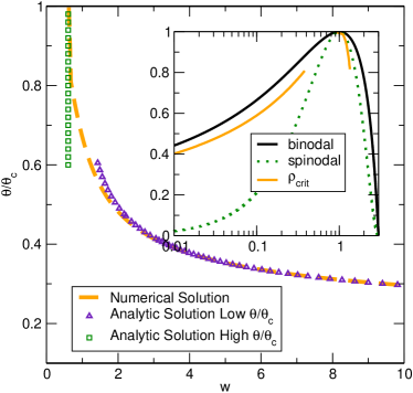
Figure 1: (Color online) The two limiting cases for which we can obtain an analytical approximation to the $w(\kappa_{m})$ relation. The inset shows the value of the critical density $\rho_{crit}$, which is the value $\rho_{s}$ takes when (3) is maximized. Note that there is a discontinuity.

We first examine numerically which values of $\rho_{s}$ in Eq. (3) lead to the most restrictive constraint, i.e. the largest value of $\kappa_{m}(\rho_{s})$. The orange line in the inset of Figure 1 shows how this density $\rho_{crit}$ varies as a function of temperature. Near to the critical temperature, the orange line in the inset in Figure 1 lies close to the high density spinodal curve. This is because $P-p_{b}$ has its highest magnitude here, therefore helping to maximize $\kappa_{m}$ within this region. An analytical estimate for $\kappa_{m}$ can be obtained by expanding the pressure around the critical density, giving

$$P-p_{b}=-\frac{9}{4}\left(\theta_{c}-\theta\right)\left(\rho_{s}-1\right)+\frac{3}{16}\left(\rho_{s}-1\right)^{3}.$$ (8)

Within this regime, $P-p_{b}$ is large and negative, therefore $\rho_{-}$ and $\rho_{+}$ must be chosen to make the denominator in (3) as negative as possible. A suitable choice is $\rho_{-}$ = $\rho_{g}$ and $\rho_{+}$ = $\rho_{s}$. We assume that the critical value of $\rho_{s}$ lies on the spinodal curve $\rho_{spin}=1+2\sqrt{\theta_{c}-\theta}$. This allows us to obtain $\kappa_{m}$, and substituting this expression into (7) gives a minimum interface width of

$$w_{min}=\frac{1}{\sqrt{1+\sqrt{3}}}.$$ (9)

As the temperature is decreased in the inset of Figure 1 the critical density $\rho_{crit}$ makes a discontinuous jump to a regime in which it lies close to the gas density, $\rho_{g}$. The minimum interface width can, in this case, be analytically obtained by expanding densities around $\rho_{g}$. We define $\rho_{s}=\rho_{g}+\delta\rho$ and $\rho_{+}=\rho_{-}+\Delta\rho$. Since $P-p_{b}$ is a positive quantity, a suitable choice for $\rho_{-}$ is $\rho_{-}=\rho_{s}$. Substituting these expressions into equation (3) gives

$$\kappa_{m}=\max_{\delta\rho>0}\min_{\Delta\rho>0}\frac{\theta\delta\rho}{(\rho_{g}+\delta\rho)\Delta\rho-\Delta\rho^{2}/8},$$ (10)

Minimizing this with respect to $\Delta\rho$ leads to $\rho_{s}=\Delta\rho/4$. Re-substituting this result back into equation (10), and maximizing with respect to $\delta\rho$, we finally obtain $\rho_{crit}=2\rho_{g}$. Using this we can calculate the minimum interface width,

$$w_{min}=\frac{1}{\sqrt{4\rho_{g}\left(\theta_{c}-\theta\right)}},$$ (11)

as shown by the triangles in Figure 1. This closely follows the numerical result at low temperatures. This means that we need wide interfaces for deep quenches because of the unfortunate cancellation of the discrete derivative and Laplace operator for low densities in the denominator of (3).

Most previous lattice Boltzmann simulations approached the simulation of non-ideal systems by using the ideal gas equation of state $p=\rho\theta=\rho/3$, as a starting point. Interactions are then included to allow the simulation of non-ideal systems. The speed of sound $c_{s}=\sqrt{\partial_{\rho}p}$ will then recover the ideal gas value of $1/\sqrt{3}$ in the dilute limit. For a van der Waals gas with a critical density of 1 and a temperature of $\theta=1/3$ and an interfacial free energy of $\int\kappa/2\;(\nabla\rho)^{2}$ the pressure tensor used by previous approaches matched the ideal gas equation of state in the dilute limit, leading to $p_{0}=1$. For the van der Waals gas the speed of sound increases rapidly for high densities. A problem arises when the speed of sound becomes larger then the lattice velocity $|v_{i}|$, because information can not be passed on at speeds larger than the lattice velocity. When the speed of sound is increased above 1 the simulation becomes unstable. This problem is exacerbated by the presence of the gradient terms in the pressure tensor. These terms further decrease the stability, as shown in a previous analysis of the pressure method by C. Pooley for one, two, and three dimensional lattice Boltzmann methods PooleyThesis . In the notation of this letter the linear stability condition is

$$c_{s}<\sqrt{1-4p_{0}\kappa\rho}$$ (12)

for a homogeneous, one dimensional system with density $\rho$. This implies a restriction for both the maximum quench depth and the maximum intereface witdth. This is shown in Fig. 3 as solid lines for different values of $p_{0}$. This suggests that, at least as far as the stability of the bulk phase is concerned, the most stable solutions should be found for $\kappa=0$.

For simplicity we demonstrate the constraints of liquid-gas lattice Boltzmann simulations by the common one dimensional projection of one, two and three dimensional models. This is the D1Q3 model. The lattice Boltzmann equation for densites $f_{i}$ corresponding to velocity $v_{i}$ is given by

$$f_{i}(\mathbf{x}+\mathbf{v}_{i},t+1)=f_{i}(\mathbf{x},t)+\frac{1}{\tau}(f_{i}^{0}(\mathbf{x},t)-f_{i}(\mathbf{x},t)).$$ (13)

The $f_{i}^{0}$ are the equilibrium distribution and are given by

$$f_{-1}=-\rho u/2+\Pi/2;\;f_{0}=\rho-\Pi;\;f_{1}=\rho u/2+\Pi/2$$

and $\Pi=\rho u^{2}+P+\nu u\partial_{x}\rho$ Holdych ; pre where $\nu=(\tau-0.5)/3$. To second order the resulting equations of motion are, as usual, the continuity equation

$$\partial_{t}\rho+\partial_{x}(\rho u)=0$$ (14)

and the Navier Stokes equation

$$\partial_{t}(\rho u)+\partial_{x}(\rho u^{2})=-\partial_{x}P+\partial_{x}(2\nu\rho\partial_{x}\rho)$$ (15)

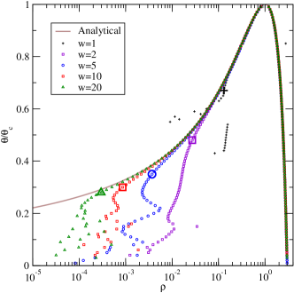
Figure 2: (Color online) The van der Waals phase diagram is recovered to very good approximation for interfaces wider than the minimum width. The large symbols represent the predicted points at which the simulations are predicted to become inaccurate by Eq. (3). The value of $p_{0}$ only affects the bulk stability and values from 1 to $10^{-7}$ were used for increasing quench depth.

To lower the speed of sound in the liquid phase we now reduce the value of $p_{0}$ in (5). This decreases the speed of sound in the liquid by a factor $\sqrt{p_{0}}$. This also increases the range of stability for $\kappa$ in (12). We now expect that lowering the speed of sound by a sufficient factor will reduce the speed of sound sufficiently to simulate systems with arbitrarily low temperature ratios $\theta/\theta_{c}$.

To test this idea we performed simulations with near equilibrium profiles using a one dimensional three velocity $v_{i}=\{-1,0,1\}$ model by defining an initial density profile that is given by two domains with densities $\rho_{l}$ and $\rho_{g}$ respectively connected by an equilibrium interface given by Eq. (6). This profile is not the exact analytical solution to the differential equation $\nabla P=0$, but it is very close to it. By initializing the simulation with this profile we test the linear stability of the method around an equilibrium profile to good accuracy. The shape of a stable interfacial profile is independent of $p_{0}$.

In Figure 2 we see that by lowering $p_{0}$ the method is now able to simulate very small values of the reduced temperature $\theta/\theta_{c}$ for interface width $w>1$, but that significantly larger widths are required to recover an accurate phase diagram for deep quenches. For values of $\theta/\theta_{c}$ between 0.9 and 1 we also find non unique solutions for small values of $\kappa$ which is discussed in more detail in a previous paper pre .

We now test the predictions of the accuracy of extended interface liquid-gas simulations using a lattice Botzmann implementation first presented in pre .

For small values of $\kappa$ the interface becomes sharp in the continuous limit so that the derivatives become arbitrarily large. But in the numerical implementation the derivatives are discrete. The discrete values are limited by the lattice spacing. In the one dimensional case we choose $\nabla\rho(x)=0.5(\rho(x+1)-\rho(x-1))$ and $\nabla^{2}\rho(x)=\rho(x+1)-2\rho(x)+\rho(x-1)$.

The methods always lead to a constant pressure, even across an interfacepre . We performed a scan of the parameter space $w$ and $\theta/\theta_{c}$ initializing the simulation with a near equilibrium profile for different values of $p_{0}$. We accept simulations that are stable, accurate and unique. The criterion of accuracy is defined to be $\log_{10}(\rho_{min})-\log_{10}(\rho_{g})<0.1$. As can be seen in Figure 2, the results are not very sensitive to the exact value of the cutoff. For values of the interface width $w<1.5$ we also test the uniqueness of the simulation by using initial profiles with bulk densities corresponding to the pressure at the spinodal pointspre . Our criterion for uniqueness is that all simulations lead to the same minimum density to within $\Delta\rho<0.01$.

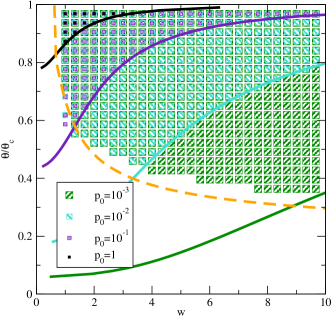
Figure 3: (Color online) Existence of accurate solutions for different values of $p_{0}$ and $w$. Symbols indicate parameter combinations that lead to stable, accurate, and unique solutions. Solid lines are the bulk stability limits for the pressure method given by Eq. (12). The dashed line is the line for an accurate interface representation given by Eq. (3).

Comparing (3), shown as a dashed line in Figure 3, and the numerical results for stable, accurate and unique solutions shows excellent agreement. The bulk stability of Eq. (12) gives the second limit for the acceptable parameter range for the pressure method. We perforemd a similar analysis for the forcing method of pre and obtained nearly identical results except for a slightly larger range of bulk stability. Note that previous lattice Boltzmann simulations use $p_{0}=1$, which corresponds to the area under the black line in Fig. 3. This is why it was assumed that lattice Boltzmann simulations are limited to a maximum density ratio of about 10 Inamuro .

The interface constraint (3) is remarkably successful at predicting the acceptable simulation parameters. It predicts how thin is too thin for an interface. It thereby detects when non-unique solutions occur and when solutions for deep quenches fail to deliver accurate results.

For simulation methods it is important to be aware of the acceptable paramter ranges. Lattice Boltzmann simulations are often believed to have the nice property of becoming unstable before they become inaccurate cates . This is not the case for thin interfaces in multi-phase simulations. In this case the simulation can remain stable and become inaccurate. This makes it necessary to find some criterion that determines whether a set of paramters will lead to an accurate simulation. Such a criterion was presented for the interface width (controlled by $\kappa$) in this communication.

The second contribution presented in this paper appears trivial at first: in consists of a simple pre-factor for the pressure. It is new, because it breaks with the idea that the standard lattice Boltzmann method for ideal gases should always be recovered in the dilute limit. This prefactor has profound implications on the stability of the bulk phases, which can be seen using an important result about the bulk stability from PooleyThesis .

Combining these two components we were able to show that lattice Boltzmann is indeed able to simulate very deep quenches for liquid-gas cases. This analysis was general and will be applied to other equation of states as well as other discretization of the interfacial terms. This may yet yield significant further advances for the development of multi-phase lattice Boltzmann methods.

References

- (1) T. Inamuro, T. Ogata, S. Tajima, N. Konishi, J. Comp. Phys.198, 628 (2004).
- (2) M.R. Swift, W.R. Osborn and J.M. Yeomans, Phys. Rev. Lett 75,(1995), M.R. Swift, E. Orlandini, W.R. Osborn and J.M. Yeomans, Phys. Rev. E 54, 5041 (1996).
- (3) D.J. Holdych, D. Rovas, J.G. Georgiadis, R.O. Buckius, Int. J. of Mod. Phys. C 9, 1393 (1998).
- (4) T. Inamuro, N. Konishi, F. Ogino, Comp. Phys. Comm. 129 32 (2000).
- (5) A.N. Kalarakis, V.N. Burganos and A.C. Payatakes, Phys. Rev. E 65, 056702 (2002), A.N. Kalarakis, V.N. Burganos and A.C. Payatakes, Phys. Rev. E 67, 016702 (2003).
- (6) X. Shan and H. Chen, Phys. Rev. E 47, 1815 (1993).
- (7) X. He, X. Shan and G.D. Doolen, Phys. Rev. E 57, R13 (1998).
- (8) L-S. Luo, Phys. Rev. Lett. 81, 1618 (1998).
- (9) V. Sofonea and K.R. Mecke, Euro. Phys. J. B 8, 99 (1999).
- (10) X. Jia, J.B. McLaughlin, and K. Kontomaris, Physica A 326, 62 (2006).
- (11) H. Kusumaatmaja, A. Dupius, J.M. Yeomans, Math. and Comp. in Simul. 72, 160 (2006).
- (12) D. Grubert, J.M. Yeomans, Comp. Phys. Comm. 121, 236 (1999).
- (13) A.J. Briant, A.J. Wagner, J.M. Yeomans, Phys. Rev. E 69, 031602 (2004).
- (14) J. Zhang, D.Y. Kwok, Langmuir 20, 8137 (2004).
- (15) A.J. Wagner, submitted to Phys. Rev. E, preprint available at cond-mat/0607087.
- (16) A.J. Wagner and Q. Li, Physica A 362, 105 (2005).
- (17) Christopher M. Pooley, “Mesoscopic modelling techniques for complex fluids”, thesis, Oxford University, 2003.
- (18) V. M. Kendon and M. E. Cates and J.-C. Desplat and I. Pagonabarraga and P. Bladon, J. Fluid Mech. 440, 147 (2001).