Thermodynamic quantum critical behavior of the Kondo necklace model

Abstract

We obtain the phase diagram and thermodynamic behavior of the Kondo necklace model for arbitrary dimensions $d$ using a representation for the localized and conduction electrons in terms of local Kondo singlet and triplet operators. A decoupling scheme on the double time Green’s functions yields the dispersion relation for the excitations of the system. We show that in $d\geq 3$ there is an antiferromagnetically ordered state at finite temperatures terminating at a quantum critical point (QCP). In 2-d, long range magnetic order occurs only at $T=0$. The line of Neel transitions for $d>2$ varies with the distance to the quantum critical point QCP $|g|$ as, $T_{N}\propto|g|^{\psi}$ where the shift exponent $\psi=1/(d-1)$. In the paramagnetic side of the phase diagram, the spin gap behaves as $\Delta\approx\sqrt{|g|}$ for $d\geq 3$ consistent with the value $z=1$ found for the dynamical critical exponent. We also find in this region a power law temperature dependence in the specific heat for $k_{B}T\gg\Delta$ and along the non-Fermi liquid trajectory. For $k_{B}T\ll\Delta$, in the so-called Kondo spin liquid phase, the thermodynamic behavior is dominated by an exponential temperature dependence.

I Introduction

Quantum phase transitions from an antiferromagnetic (AF) ordered state to a non-magnetic Fermi liquid in heavy fermions (HF) systems have been the subject of intense research recentlyJulio . In contrast to classical phase transitions, driven by temperature, quantum phase transitions can be driven by magnetic field, external pressure or doping. The physics of heavy fermion compounds is mainly due to the competition of two main effects: the Ruderman-Kittel-Kasuya-Yosida (RKKY) interaction between the magnetic ions which favors long range magnetic order and the Kondo effect which tends to screen the moments and produce a non-magnetic ground state. These effects are contained in the Kondo Lattice Model (KLM) Hamiltonian Doniach which can be derived from the more fundamental Anderson lattice model in the case of well-developed local spin moments Schieffer . Although this model neglects charge fluctuations, since the relevant QCP in heavy fermion materials is associated with a magnetic transition, to consider only spin fluctuationsguang turns out an excellent approximation. The KLM has been studied by different techniques and the general physical picture that arises is that at $T=0$, there is a quantum phase transition from a magnetic phase at small coupling strength $J/t$ to a non-magnetic dense Kondo phase at a critical value of $J/t$.

Here we investigate a simplified version of this model, the so called Kondo necklace modelDoniach (KNM), which for all purposes can be considered as yielding results similar to the original model. We use the bond-operator approach introduced by Sachdev et.al. sachdev that was employed previously to both KLM jure and KNM guang models but always at zero temperature. We extend this approach to finite temperatures Da and obtain the phase diagram of the KNM for arbitrary dimensions. We find, that this method yields a critical Neel line in three dimensions but not in 2-d as expected from general argumentsMermin . This implies that fluctuations are taken into account to an important extent in spite of the mean-field type of decoupling used to deal with the bond-operator Hamiltonian. We also calculate the thermodynamic properties along the non-Fermi liquid (NFL) trajectory above the QCP Mucio1 ; Hertz ; Moriya ; Millis .

The KNM replaces the hopping term of the conduction electrons by an $X-Y$ interaction among the conduction electron spins Doniach . It is given by,

$$H=t\sum_{<i,j>}(\tau^{x}_{i}\tau^{x}_{j}+\tau^{y}_{i}\tau^{y}_{j})+J\sum_{i}\mathbf{S}_{i}.\mathbf{\tau}_{i},$$ (1)

where $\tau_{i}$ and $\mathbf{S}_{i}$ are independent sets of spin-1/2 Pauli operators, representing the conduction electron spin and localized spin operators, respectively. The sum $\langle i,j\rangle$ denotes summation over the nearest-neighbor sites. The first term mimics electron propagation and in one dimension can be mapped by the Jordan-Wigner transformation onto a band of spinless fermions. The second term is the magnetic interaction between conduction electrons and localized spins $\mathbf{S}_{i}$ via the coupling $J$.

The paper is organized as follows: In Sec. II we introduce the bond operator treatment of the KNM. In Sec. III we make and discuss the approximations required to solve the problem. The Green’s function method is employed to attain this solution, as it can be easily generalized to finite temperatures. We obtain a closed set of equations for the Green’s functions that can be immediately solved without no further approximations. The temperature dependence of the singlet and triplet order parameters is found in Sec. IV. In Sec. V the finite temperature phase diagram of the KNM is discussed. In Sec. VI we study the paramagnetic phase and find the dependence of the spin gap with the distance to QCP. In Sec. VII the behavior of the specific heat of the KNM is presented. The last section (Sec. VIII) offers the conclusions and discussions.

II Bond operators representation

We use the method of bond operators, which has the advantage of making the connection to the lattice degrees of freedom most direct. For two $S=\frac{1}{2}$ spins, Sachdev et. al.sachdev introduced four creation operators to represent the four states in Hilbert space. This basis can be created out of the vacuum by singlet $|s\rangle$ and triplet $|t_{\alpha}\rangle=t_{\alpha}^{\dagger}|0\rangle$ ($\alpha=x,y,z$) operators. In terms of these triplet and singlet operators the localized and conduction electrons spin operators are given by,

$$S_{i,\alpha} = \frac{1}{2}(s_{i}^{\dagger}t_{i,\alpha}^{\phantom{\dagger}}+t_{i,\alpha}^{\dagger}s_{i}^{\phantom{\dagger}}-i\epsilon_{\alpha\beta\gamma}t_{i,\beta}^{\dagger}t_{i,\gamma}^{\phantom{\dagger}}),$$

$$\tau_{i,\alpha} = \frac{1}{2}(-s_{i}^{\dagger}t_{i,\alpha}^{\phantom{\dagger}}-t_{i,\alpha}^{\dagger}s_{i}^{\phantom{\dagger}}-i\epsilon_{\alpha\beta\gamma}t_{i,\beta}^{\dagger}t_{i,\gamma}^{\phantom{\dagger}}).$$ (2)

where $\alpha$, $\beta$ and $\gamma$ take the values $x$, $y$, $z$, repeated indices are summed over, and $\epsilon$ is the totally antisymmetric Levi-Civita tensor. In particular, an important feature of the bond operator mean-field approach is that the simplest mean-field theory to be used below already yields ground states and excitations with the correct quantum numbers; so a strong fluctuation analysis is not needed to capture the proper physics. The restriction that the physical states are either singlets or triplets leads to the constraint $s^{\dagger}s+\sum_{\alpha}t_{\alpha}^{\dagger}t_{\alpha}=1$. Moreover, the singlet and triplet operators at each site satisfy bosonic commutation relations $[s,s^{\dagger}]=1,[t_{\alpha},t_{\beta}^{\dagger}]=\delta_{\alpha,\beta},[s,t_{\alpha}^{\dagger}]=0$. Substituting the operator representation of spins defined in Eq. (2) into the original Hamiltonian and considering the commutation relations, we obtain

$$H=H_{0}+H_{1}+H_{2}$$

where

$$H_{0} = \frac{J}{4}\sum_{i}(-3s_{i}^{\dagger}s_{i}^{\phantom{\dagger}}+\sum_{\alpha}t_{i,\alpha}^{\dagger}t_{i,\alpha}^{\phantom{\dagger}})$$

$$+ \sum_{i}\mu_{i}(s_{i}^{\dagger}s_{i}^{\phantom{\dagger}}+\sum_{\alpha}t_{i,\alpha}^{\dagger}t_{i,\alpha}^{\phantom{\dagger}}-1),$$

$$H_{1} = \frac{t}{4}\sum_{\langle ij\rangle,\alpha}\left[s_{i}^{\dagger}s_{j}^{\dagger}t_{i,\alpha}^{\phantom{\dagger}}t_{j,\alpha}^{\phantom{\dagger}}\right.+\left.s_{i}^{\dagger}s_{j}^{\phantom{\dagger}}t_{i,\alpha}^{\phantom{\dagger}}t_{j,\alpha}^{\dagger}+h.c.\right],$$

$$H_{2} = -\frac{t}{4}\sum_{\langle ij\rangle,\alpha}\left[t_{i,z}^{\dagger}t_{j,z}^{\dagger}t_{i,\alpha}^{\phantom{\dagger}}t_{j,\alpha}^{\phantom{\dagger}}\right.-\left.t_{i,z}^{\dagger}t_{j,z}^{\phantom{\dagger}}t_{i,\alpha}^{\phantom{\dagger}}t_{j,\alpha}^{\dagger}+h.c.\right].$$

with $\alpha=x,y$. $H_{0}$ represents the interaction between spins $S$ and $\tau$ in the site $i$ and the constraint $s^{\dagger}s+\sum_{\alpha}t_{\alpha}^{\dagger}t_{\alpha}=1$ is implemented through the local chemical potentials $\mu_{i}$. $H_{1}$ and $H_{2}$ are terms associated with the hopping. There is still another term in the Hamiltonian that consists of three triplets and one singlet operator. This is not taken into account since it vanishes in the approximation that we use below guang .

III Antiferromagnetic Phase

The Hamiltonian above, at half filling, i.e., with one conduction electron per site, can be simplified using a mean-field decoupling of the quartic terms while still retaining the relevant physics. The resulting effective Hamiltonian $H_{mf}$ with only quadratic operators is sufficient to describe exactly the quantum phase transition from the ordered AF state to the disordered Kondo spin liquid at least for $d\geq 3$, as discussed below. Besides it also yields sensible results in 2-d where no line of finite temperature transitions is found. Relying on the nature of the strong coupling limit $(t/J)\rightarrow 0$ we take $\langle s_{i}^{\dagger}\rangle=\langle s_{i}\rangle=\overline{s}$, which corresponds to a condensation of the local Kondo spin singlets on each site . Next to describe the condensation of one local Kondo spin triplet $t_{\mathbf{k},x}$ on the AF reciprocal vector $Q=(\pi/a,\pi/a,\pi/a)$, we introduce: $t_{\mathbf{k},x}=\sqrt{N}\bar{t}\mathbf{\delta_{k,Q}}+\mathbf{\eta}_{\mathbf{k},x}$ corresponding to fixing the orientation of the localized spins along the $x$ direction. The quantity $\bar{t}$ is the mean value of the $x$-component spin triplet in the ground state and $\mathbf{\eta}_{\mathbf{k},x}$ represents the fluctuations. Finally the translation invariance of the problem implies that we may assume the local chemical potential as a global one.

We will consider here only the terms $H_{0}$ and $H_{1}$; the $H_{2}$ term has only small contributions to the results therefore it is neglectedRice ; Normand .

After performing a Fourier transformation of the boson operators, the mean-field effective Hamiltonian is given by,

$$H_{mf}=N\left(-\frac{3}{4}J\text{ }\overline{s}^{2}+\mu\overline{s}^{2}-\mu\right)$$

$$+\left(\frac{J}{4}+\mu\right)\sum_{{\bf k}}t_{{\bf k},z}^{\dagger}t_{{\bf k},z}^{\phantom{\dagger}}+(\frac{J}{4}+\mu-\frac{1}{2}tZ\overline{s}^{2})N\bar{t}^{2}$$

$$+\sum_{\bf k}\left[\Lambda_{{\bf k}}\eta_{{\bf k},x}^{\dagger}\eta_{{\bf k},x}^{\phantom{\dagger}}+\Delta_{{\bf k}}\left(\eta_{{\bf k},x}^{\dagger}\eta_{-{\bf k},x}^{\dagger}+\eta_{{\bf k},x}\eta_{-{\bf k},x}\right)\right]$$

$$+\sum_{\bf k}\left[\Lambda_{{\bf k}}t_{{\bf k},y}^{\dagger}t_{{\bf k},y}^{\phantom{\dagger}}+\Delta_{{\bf k}}\left(t_{{\bf k},y}^{\dagger}t_{-{\bf k},y}^{\dagger}+t_{{\bf k},y}t_{-{\bf k},y}\right)\right],$$

with $\Lambda_{{\bf k}}=\omega_{0}+2\Delta_{{\bf k}}$, $\lambda({\bf k)=}\sum_{s=1}^{d}\cos k_{s}$, $\Delta_{{\bf k}}=\frac{1}{4}t\overline{s}^{2}\lambda({\bf k)}$, $N$ is the number of lattice sites, $Z$ is the total number of the nearest neighbors on the hyper-cubic lattice. The wave-vectors $k$ are taken in the first Brillouin zone and the lattice spacing was assumed to be unity. This mean-field Hamiltonian can be solved using the Green’s functions to obtain the thermal averages of the singlet and triplet correlation functions. These are given by,

$$\ll t_{{\bf k},\alpha}^{\phantom{\dagger}};t_{{\bf k},\alpha}^{{\dagger}}\gg_{\omega}=\frac{1}{2\pi}\frac{\omega+\Lambda_{{\bf k}}}{\omega^{2}-\omega_{{\bf k}}^{2}},$$ (5)

$$\ll t_{{\bf k},z}^{\phantom{\dagger}};t_{{\bf k},z}^{{\dagger}}\gg_{\omega}=\frac{1}{2\pi}\frac{1}{\omega-\omega_{0}}.$$ (6)

where, $\alpha=x,y$. The poles of the Green’s functions determine the excitation energies of the system as $\omega_{0}=\left(\frac{J}{4}+\mu\right)$, which is the dispersionless spectrum of the longitudinal spin triplet states and $\omega_{k}=\pm\sqrt{\Lambda_{{\bf k}}^{2}-(2\Delta_{{\bf k}})^{2}}$ that correspond to the excitation spectrum of the transverse spin triplet states for both branches $\omega_{x}=\omega_{y}$. From these modes and their bosonic character an expression for the average energy at finite temperatures can be easily obtained,

$$\varepsilon=\langle\mathcal{H}_{mf}\rangle = \varepsilon_{0}+\frac{\omega_{0}}{2}\sum_{\mathbf{k}}\left(\coth\frac{\beta\omega_{0}}{2}-1\right)$$ (7)

$$+ \sum_{\mathbf{k}}\omega_{\mathbf{k}}\left(\coth\frac{\beta\omega_{\mathbf{k}}}{2}-1\right),$$

where

$$\varepsilon_{0} = N\left[-\frac{3}{4}J\overline{s}^{2}+\mu\overline{s}^{2}-\mu+\left(\frac{J}{4}+\mu-\frac{1}{2}tZ\overline{s}^{2}\right)\overline{t}^{2}\right]$$ (8)

$$+ \sum_{\mathbf{k}}(\omega_{\mathbf{k}}-\omega_{0}),$$

is the ground state energy of the system and $\beta=1/k_{B}T$, $\overline{s}$ and $\overline{t}$ the singlet and triplet order parameter respectively. Since the parameter $\overline{s}$ is always nonzeroguang ; jure and $\overline{t}\neq 0$ in the antiferromagnetic phase, we minimize the ground state energy with respect to $\overline{t}$ to find, $\mu=\frac{1}{2}Zt\overline{s}^{2}-J/4$ and consequently, $\omega_{{\bf k}}=\frac{1}{2}Zt\overline{s}^{2}\sqrt{1+2\lambda(\mathbf{k})/Z}$. The ground state energy $\varepsilon_{0}$ corresponds to a magnetically long-range ordered state characterized by the momentum $q=Q$. The excitations over this ground state are given by two spin-wave branches associated with $t_{x}$ and $t_{y}$ that represent rotations or transverse oscillations of the order parameter $\bar{t}$. The third mode associated with $t_{z}$ corresponds to fluctuations in the amplitude of this order parameter. In the next section we consider low temperatures with the purpose of studying the behavior of the system near the magnetic instability.

IV Singlet and triplet order parameters at finite temperatures

The low temperature thermodynamic and transport properties of heavy fermions in the vicinity of the magnetic quantum critical point are far from being completely understood Mucio2 . In order to study the KNM at finite temperatures we calculate in this section the finite temperature order parameters $\overline{s}^{2}=\overline{s}^{2}(T)$ and $\overline{t}^{2}=\overline{t}^{2}(T)$. The free energy can be directly obtained from the energy of the excitations given by the poles of the Green’s functions found in the previous section. It is given by,

$$G=\varepsilon_{0}-\frac{2}{\beta}\sum_{\mathbf{k}}\ln[1+n(\omega_{\mathbf{k}})]-\frac{N}{\beta}\ln[1+n(\omega_{0})]$$ (9)

where

$$n(\omega)=\frac{1}{2}\left(\coth\frac{\beta\omega}{2}-1\right)$$ (10)

Minimizing the free energy of the KNM using $(\partial\varepsilon/\partial\mu,\partial\varepsilon/\partial\overline{s})=(0,0)$, we can easily get the following saddle-point equations,

$$\overline{s}^{2} = 1+\frac{J}{Zt}-\frac{1}{2N}\sum_{\mathbf{k}}\sqrt{1+\frac{2\lambda(\mathbf{k})}{Z}}\coth\frac{\beta\omega_{\mathbf{k}}}{2}-\xi,$$

$$\overline{t}^{2} = 1-\frac{J}{Zt}-\frac{1}{2N}\sum_{\mathbf{k}}\frac{1}{\sqrt{1+\frac{2\lambda(\mathbf{k})}{Z}}}\coth\frac{\beta\omega_{\mathbf{k}}}{2}-\xi.$$

where $\xi=\frac{1}{4}(\coth\frac{\beta\omega_{0}}{2}-1)$. Generally the equations for $\overline{s}$ and $\overline{t}$ in Eq. (IV) should be solved and at $T=0$ the results of Ref. (4) are recovered. For $J/t>(J/t)_{c}$, triplet excitations remain gapped and at $J/t<(J/t)_{c}$, the ground state has both condensation of singlets and triplets at the antiferromagnetic wave vector $Q=(\pi,\pi,\pi)$. Then the quantum critical point at $T=0$, $(J/t)_{c}$ separates an antiferromagnetic long range ordered phase from a gapped spin liquid phase. For finite temperatures, the condensation of singlets $s$ occurs at a temperature scale which, to a first approximation, tracks the exchange $J$. The energy scale below which the triplet excitations condense is given by the Neel temperature ($T_{N}$) which is calculated in the next section.

V Critical Neel line in the KNM

In terms of the KNM, the condensation of triplets (singlets) follows from the RKKY interaction (Kondo effect). Thus, the fact that at the mean-field level, both $\overline{s}$ and $\overline{t}$ do not vanish may be interpreted as the coexistence of Kondo screening and antiferromagnetism in the ordered phaseguang ; jure for all values of the ratio $J/t<(J/t)_{c}$. Notice that the bond-operator mean-field theory is appropriate in the strong coupling limit and near the QCP. However it does not give an accurate description of the weak limit for $(J/t)\rightarrow 0$, where the ground state is macroscopically degenerate.

The Neel line giving the finite temperature instability of the antiferromagnetic phase for $J/t<(J/t)_{c}$ is obtained as the line in the $T$ vs $(J/t)$ plane at which $\overline{t}$ vanishes ($\overline{t}=0$). From Eq. (IV) we can then obtain the boundary of the AF state. From this equation we get,

$$\frac{|g|}{Z}=\frac{1}{2N}\sum_{\mathbf{k}}\frac{1}{\sqrt{1+\frac{2\lambda(\mathbf{k})}{Z}}}\left(\coth\frac{\beta\omega_{\mathbf{k}}}{2}-1\right)+\xi,\\$$ (12)

where $g=|(J/t)_{c}-(J/t)|$ measures the distance to the QCP. The latter is given by, $(J/t)_{c}=Z[1-\frac{1}{2N}\sum_{\mathbf{k}}\frac{1}{\sqrt{1+2\lambda(\mathbf{k})/Z}}]$ where $Z$ is the number of nearest neighbors. Expanding close to the wave-vector $\mathbf{Q}=(\pi,\pi,\pi)$ associated with the antiferromagnetic instability we get,

$$\lambda(\mathbf{k})=-d+\frac{k^{2}}{2}+O(k^{4}),$$ (13)

This yields the spectrum of transverse spin triplet excitations as,

$$\omega_{\mathbf{k}}=\omega_{0}\sqrt{1+\frac{2\lambda(\mathbf{k})}{Z}}\approx\sqrt{D}k.$$ (14)

where $\sqrt{D}=\omega_{0}/\sqrt{2d}$, with $\omega_{0}$ the z-polarized dispersionless branch of excitations and $d$ is the Euclidean dimension. Notice that the low temperature specific heat in the antiferromagnetic phase is dominated by the contribution of these modes. In $3d$ this has a $T^{3}$ temperature dependence due to the linear, phonon-like, dispersion relation.

Replacing Eq. (14) in Eq. (12) and considering that for temperatures $k_{B}T\ll\omega_{0}$, $\xi$ goes to zero faster than the first term of Eq. (12) we obtain,

$$\frac{|g|}{Z} = \frac{2^{d-2}S_{d}Z^{d/2}}{\pi^{d}}\left(\frac{k_{B}T}{\omega_{0}}\right)^{d-1}$$ (15)

$$\times \int_{0}^{\frac{\pi}{2\sqrt{Z}}\frac{\omega_{0}}{k_{B}T}}u^{d-2}\left(\coth u-1\right)du,\$$

where $S_{d}$ is the solid angle and $u=\beta\omega_{0}k/2\sqrt{Z}$. For temperatures $k_{B}T\ll\omega_{0}$ the integral in Eq. (15) can be calculated and we get

$$\frac{|g|}{Z}=\frac{2^{d-2}S_{d}Z^{d/2}}{\pi^{d}\omega_{0}^{d-1}}(k_{B}T_{N})^{d-1}f(d),$$ (16)

where $f(d)=\int_{0}^{\infty}u^{d-2}\left(\coth u-1\right)du$. The solution of this expression gives us the critical line of Neel transitions for any dimension and temperatures $k_{B}T\ll\omega_{0}$ where $\omega_{0}=(\frac{J}{4}+\mu)$ is the dispersionless spectrum of the longitudinal spin triplet states that tracks $J$. We notice that the integral $f(d)$ diverges for $d<3$ showing that there is no critical line in two dimensions at finite temperaturesDa , in agreement with the Mermin-Wagner theoremMermin . For $d\geq 3$, $f(d)$ is finite and the equation for the critical line is given by,

$$T_{N}\propto|g|^{\frac{1}{d-1}},$$ (17)

which defines a shift exponent $\psi=1/(d-1)$. In particular for $3d$, $f(3)=\pi^{2}/12$ and the critical line of Neel is given by $k_{B}T_{N}=0.13\omega_{0}|g|^{1/2}$. In summary, in this section we have obtained analytically the expression for the Neel line close to the QCP and we have shown that this line does not exist for $d=2$ as expected.

VI Paramagnetic phase

Our interest here is to obtain the thermodynamic properties near, but above the QCP, i.e., for finite temperatures in the spin liquid phase for $J/t\geq(J/t)_{c}$. In this case we have to consider only the condensation of singlets since $\overline{t}=0$ in the paramagnetic phase. We find,

$$\varepsilon^{\prime} = \ \varepsilon^{\prime}_{0}+\frac{\omega_{0}}{2}\left(\coth\frac{\beta\omega_{0}}{2}-1\right)$$ (18)

$$+ \sum_{\mathbf{k}}\omega_{\mathbf{k}}\left(\coth\frac{\beta\omega_{\mathbf{k}}}{2}-1\right),$$

The ground state energy is now given by $\varepsilon^{\prime}_{0}=N\left(-\frac{3}{4}J\text{ }\overline{s}^{2}+\mu\overline{s}^{2}-\mu\right)+\sum_{\mathbf{k}}\left(\omega_{\mathbf{k}}-\omega_{0}\right)$ and the free energy by,

$$G^{\prime}=\varepsilon^{\prime}_{0}-\frac{2}{\beta}\sum_{\mathbf{k}}\ln[1+n(\omega_{\mathbf{k}})]-\frac{N}{\beta}\ln[1+n(\omega_{0})]$$ (19)

The transverse spin triplet excitation spectrum can be expressed in the general form ${\omega_{{\bf k}}}=\sqrt{\Lambda_{{\bf k}}^{2}-(2\Delta_{{\bf k}})^{2}}$, where the excitations are triply degenerate magnons (triplons) with a spin gap that vanishes on approaching the QCP, as we show below.

We minimize the paramagnetic KNM free energy, deriving the following saddle-point equations:

$$2J\left(\frac{3}{4}-\frac{\mu}{J}\right) = \frac{t}{N}\sum_{\mathbf{k}}\frac{\omega_{0}}{\omega_{{\bf k}}}\lambda({\bf k)}\coth\frac{\beta\omega_{{\bf k}}}{2},$$

$$2-\overline{s}^{2} = \frac{1}{N}\sum_{\mathbf{k}}\frac{\Lambda_{{\bf k}}}{\omega_{{\bf k}}}\coth\frac{\beta\omega_{{\bf k}}}{2}+2\xi.$$ (20)

At $T=0$ the self-consistent equations above are equivalent to those found in the Kondo spin liquid ground stateguang . Considering again the expansion close to the QCP of Eq. (13), we obtain the transverse spin triplet excitation spectrum in the paramagnetic phase as,

$${\omega_{{\bf k}}}=\sqrt{\Delta^{2}+Dk^{2}}.$$ (21)

These quasi-particle excitations form a band whose bandwidth is a function of $t$. The band-minimum is at $k=\pi$ and the triplet excitation spectrum has a spin gap given by,

$$\Delta=\omega_{0}\sqrt{1-\frac{yZ}{2}},$$ (22)

In Eq. 21, $D=y\omega_{0}^{2}/2$ and $y=t\overline{s}^{2}/\omega_{0}$ is a dimensionless parameter. The spin gap decreases as the hopping $t$ (hence $y$) increases and vanishes when $y\rightarrow 2/Z$.

VI.1 Dependence of the spin gap on the distance to the QCP

We now obtain the dependence of the spin gap $\Delta$ with the distance to QCP, given by $g=|J/t-(J/t)_{c}|$, in the quantum disordered Kondo spin liquid state from Eq. (VI) at $T=0$. This was done previously for the spin gap in spin ladder systems but always in one dimensionRice ; Dagotto .

The first step is to express Eq. (VI) as an equation for the parameter $y$,

$$y=2\left(\frac{t}{J}\right)\left[1-\frac{S_{d}}{2^{1-d}\pi^{d}}\frac{1}{\sqrt{1+yd}}K(\eta)\right],$$ (23)

with

$$K(\eta)=\int_{0}^{\pi/2}\frac{\theta^{d-1}d\theta}{\sqrt{1-\eta^{2}\sin^{2}{\theta}}},$$ (24)

where $\eta=\sqrt{2yd/(yd+1)}$ and $K(\eta)$ in one dimension is the complete elliptic integral of the first kindRice . In Eq. (22) we see that when $y=y_{c}=2/Z$, the spin gap vanishes yielding

$$\left(\frac{J}{t}\right)_{c}=\frac{2}{y_{c}}\left[1-\frac{S_{d}}{2^{1-d}\pi^{d}}\frac{1}{\sqrt{1+y_{c}d}}K\left(\eta_{c}\right)\right],$$ (25)

where $\eta_{c}=\sqrt{2y_{c}d/(y_{c}d+1)}$. Since $|g|=|J/t-(J/t)_{c}|$ we obtain,

$$\frac{2(y_{c}-y)}{y_{c}y}=|g|+\frac{S_{d}2^{d}}{\pi^{d}}G(y),$$ (26)

where

$$G(y)=\frac{1}{y\sqrt{1+yd}}K(\eta)-\frac{1}{y_{c}\sqrt{1+y_{c}d}}K(\eta_{c}),$$ (27)

The above equation can be expanded in Taylor’s series for $y$ near $y_{c}$ yielding,

$$G(y)\approx\frac{\partial}{\partial y}\frac{1}{y\sqrt{1+yd}}K(\eta)|_{y=y_{c}}(y-y_{c})+O(y-y_{c})^{2},$$ (28)

Now considering Eq. (26) we can express the spin gap energy by,

$$\Delta=J\left(\frac{1}{4}+\frac{\mu}{J}\right)\sqrt{\frac{yZ|g|}{2\left(Z+\zeta(y_{c},d)\right)}},$$ (29)

where $\zeta(y_{c},d)=\frac{S_{d}2^{d}}{\pi^{d}}\frac{\partial}{\partial y}\frac{1}{\sqrt{1+yd}}K(\eta)|_{y=y_{c}}$ with $\zeta(y_{c},2)\approx 297.01$ and $\zeta(y_{c},3)\approx 17.78$ in two and three dimensions respectively. $\mu/J$ and $y$ are given by the self-consistent equations (VI) and (23), respectively and are never critical. This relation between the spin gap and $|g|$ shows that when $(J/t)$ decreases from its strong coupling limit, the triplet gap at the wave vector $k=(\pi,\pi,\pi)$ decreases, and vanishes at $|g|=0$. Since $\Delta\propto|g|^{1/2}$, when $|g|\rightarrow 0$, we can immediately identify the gap exponent $\nu z=1/2$ at the quantum critical point of the Kondo lattice.

VII Specific Heat in the Paramagnetic phase

The purpose of this section is to consider the paramagnetic half-filled KNM energy given by Eq. (19) and discuss its finite-temperature properties near the QCP. Already the ground state and finite-temperature properties of the KLM have been intensively studied for one dimension using the density matrix renormalization group (DMRG) methodShi ; Shi1 ; Shi2 . For two dimensions this has been accomplished using finite-temperature Lanczos techniqueHaule , perturbation theoryGu and quantum Monte Carlo (QMC) simulationAssad . Lately, also for the KNM using QMC for two dimensionsAssad1 . However, less analytical work has been carried out for higher-dimensional KNM and KLM. This way, motivated by the above, we are going to analyze the specific heat $C/T\equiv\gamma$ using an analytical treatment valid for any dimension. We obtain $\gamma$ in the paramagnetic disordered phase, in two cases: First in the so called non-Fermi liquid trajectory ($|g|=0,T\neq 0$) and then, below the spin gap for $k_{B}T\ll\Delta\propto|g|^{1/2}$. We consider the free energy Eq. (19) with $\omega_{{\bf k}}=\sqrt{\Delta^{2}+Dk^{2}}$ and take into account only the contribution of the transverse spin triplet excitation spectrum $\omega_{{\bf k}}$, since the contribution of longitudinal triplet excitation $\omega_{0}$ tends to zero faster at low temperatures $k_{B}T\ll\omega_{0}\sim J$.

VII.1 Specific heat along the NFL trajectory

Non Fermi-liquid behavior is often found near a magnetic QCPStewart , indicating that the NFL state in those systems may be linked to the magnetic instability at $T=0$. In this state the coefficient of the linear term of the specific heat does not saturate as expected from the Landau scenario but shows a temperature dependence as the temperature is lowered. Exactly at the QCP, this may occur down to the lowest temperatures livroM . Next, we are going to find analytically $C/T$ at the NFL trajectory. From Eq. (19) and using $C/T=-\partial^{2}G^{\prime}/\partial T^{2}$ we get,

$$C/T=\frac{k_{B}^{2}S_{d}}{D^{d/2}2\pi^{d}}\varsigma(d)(k_{B}T)^{d-1},$$ (30)

where

$$\varsigma(d)=\int_{x_{0}}^{\sqrt{x_{0}^{2}+D\beta^{2}\pi^{2}}}u^{3}(u^{2}-x_{0}^{2})^{\frac{d-2}{2}}(\coth^{2}\frac{u}{2}-1)du,\\$$

with $x_{0}=\Delta/k_{B}T$, $\Delta=\omega_{0}\sqrt{yZ|g|/[2\left(Z+\zeta(y_{c},d)\right)]}$, $u=\sqrt{x_{0}^{2}+D\beta^{2}k^{2}}$ and $g=|(J/T)-(J/T)_{c}|$ measures the distance to the QCP. Equation (30) yields the expression for the specific heat in the paramagnetic region and it is due, as already we pointed out, to the contribution of bosons $t_{x}$ and $t_{y}$. At $|g|=0$ and low temperatures, such that, $J\gg k_{B}T\gg\Delta$ (NFL trajectory) we can rewrite Eq. (30) as follows,

$$C/T|_{|g|=0}=\gamma_{|g|=0}=\frac{S_{d}k_{B}^{2}\varsigma(|g|=0,d)}{D^{d/2}2\pi^{d}}(k_{B}T)^{d-1},$$ (31)

where $\varsigma(|g|=0,d)=\int_{0}^{\infty}u^{d+1}(\coth^{2}\frac{u}{2}-1)du$ is $24\zeta(3)$ and $16\pi^{4}/15$ in two and three dimensions, respectively and $\zeta$ is the Riemann zeta-function. Thereby $C/T\propto T^{d-1}$ at the QCP. Notice that this is consistent with the general scaling result $C/T\propto T^{(d-z)/z}$ with the dynamic exponent taking the value livroM $z=1$ . Together with the previous result for the gap exponent $\nu z=1/2$, we find that $\nu=1/2$, a result in agreement with the mean-field or Gaussian character of the approximations we have used to deal with the bond-operator Hamiltonian. Furthermore, since $z=1$, in three dimensions $d_{eff}=d+z=d_{c}=4$ where $d_{c}$ is the upper critical dimension for the magnetic transition livroM . Consequently, the present approach yields the correct description of the quantum critical point of the KNM for $d\geq 3$.

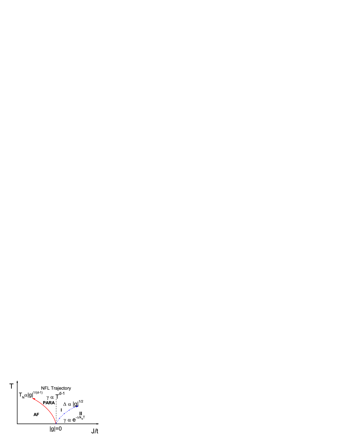
Figure 1: (Color online) Schematic phase diagram of the Kondo necklace model at finite temperatures. The AF phase is located below the Neel line $T_{N}$ (solid line), which vanishes at a critical value $(J/t)_{c}$ (QCP). The spin gap energy (dashed line) is shown as a function of $g$. Below this line there is a Kondo spin liquid state. The temperature dependence of the specific heat $\gamma=C/T$ is given along the NFL trajectory and in the Kondo spin liquid state for any dimension. The phase diagram shows that at low temperatures a small value of $J/t$ supports the development of AF order via the RKKY interaction. If the value of $J/t$ becomes too high, the local moments are quenched by the conduction electrons and the system has a dense Kondo ground state.

VII.2 Specific heat in the Kondo spin liquid state

In the region II of the Fig. (1) we have to consider the paramagnetic contribution to the specific heat given by Eq. (18) but now taking into account that $k_{B}T\ll\Delta$. Then for $k_{B}T\ll\Delta\approx\sqrt{|g|}$ we obtain,

$$C/T=\frac{2S_{d}}{\pi^{d}D^{d/2}}\frac{\Delta^{d+2}}{k_{B}T^{3}}e^{\Delta/k_{B}T}\delta(d,T),$$ (32)

where $\cosh u_{f}=1+x_{0}^{-1}$, $x_{0}=\Delta/k_{B}T$ and $\delta(d)=\int_{0}^{u_{f}}(\sinh u)^{d-1}\cosh^{3}udu$. This can be calculated and we obtain $\delta(d=2,T)=\left(\frac{k_{B}T}{\Delta}+\frac{3}{2}(\frac{k_{B}T}{\Delta})^{2}\right)$ and $\delta(d=3,T)=\frac{\sqrt{2}}{3}\left(2(\frac{k_{B}T}{\Delta})^{3/2}+\frac{17}{5}(\frac{k_{B}T}{\Delta})^{5/2}\right)$ in two and three dimensions respectively. In this case the specific heat is governed by the exponential term and we can conclude that the dimensionality does not make much difference in thermodynamic properties. This point was also indicated using numerical methods for the $2d$ KLMHaule .

Summarizing we have

$$C/T\propto\left\{\begin{array}[]{ll}T^{d-1}&\mbox{ NFL trajectory, $J\gg k_{B}T\gg\Delta$}\\ e^{-\Delta/k_{B}T}&\mbox{, $k_{B}T\ll\Delta$}\vspace{.2cm}\\ \end{array}\right.,$$ (33)

where in the latter case only the dominant term has been written. Then, we have obtained the specific heat due to the magnetic degrees of freedom in the paramagnetic phase of the half-filled KNM for any dimension and temperatures $k_{B}T\ll J$. We have investigated it in two cases: along the NFL trajectory and in the dense Kondo spin liquid phase where an exponential temperature due to the spin gap dominates over the power law associated with different dimensionalities. Unfortunately, there are few existing results in higher dimension considering the approaches done; almost all results above were obtained for the strong coupling limit ($t=0$). Our work should provide a valuable benchmark for other approaches. While we have not attempted a detailed comparison on or fit to experiment, this would be possible.

VIII Conclusions

In the present work, we have constructed analytical expressions to find the phase diagram of the Kondo necklace model for any dimension and at low temperatures, such that, $k_{B}T\ll J$. Although there were several approaches treating the Kondo lattice model with methods similar to the one we use, they were all restricted to zero temperature. The present finite temperature treatment allowed us to determine the critical line for antiferromagnetic transitions, as well as, the thermodynamic behavior along the quantum critical trajectory and in the non-critical part of the phase diagram. We obtained the relevant critical exponents governing the critical line and the thermodynamic behavior due to the magnetic degrees of freedom. For three dimensions these results turn out to be exact since $d_{eff}=d+z=4$ is equal to the upper critical dimension for the Kondo lattice.

We also found that the spin gap in the Kondo singlet phase vanishes as $\sqrt{|g|}$ at the QCP consistent with $z=1$ and a mean field correlation length $\nu=1/2$.

- (1) J. Larrea J., M. B. Fontes, E. M. Baggio-Saitovitch, J. Plessel, M. M. Abd-Elmeguid, J. Ferstl, C. Geibel, A. Pereira, A.Jornada, and M. A. Continentino, Phys. Rev. B 74, 140406(R) (2006).
- (2) S. Doniach, Physica B 91, 231 (1977).
- (3) J. R. Schrieffer and P. A. Wolff, Phys. Rev. 149, 491 (1966).
- (4) Guang-Ming Zhang, Qiang Gu and Lu Yu, Phys. Rev. B 62, 69 (2000).
- (5) S. Sachdev and R. N. Bhatt, Phys. Rev. B 41, 9323 (1990).
- (6) C. Jurecka and W. Brenig, Phys. Rev. B 64, 092406 (2001).
- (7) D. Reyes, M. A. Continentino, A. Troper and A. Saguia Physica B 359, 714 (2005).
- (8) N. D. Mermin and H. Wagner, Phys. Rev. Lett. 17, 1133 (1966).
- (9) M. A. Continentino, Phys. Rev. B 47, 11587 (1993).
- (10) J. A. Hertz, Phys. Rev. B 14, 1165 (1976).
- (11) T. Moriya and T. Takimoto, J. Phys. Soc. Jpn. 64, 960 (1995).
- (12) A. J. Millis, Phys. Rev. B 48, 7183 (1993).
- (13) S. Gopalan, T. M. Rice and M. Sigrist, Phys. Rev. B 49, 8901 (1994).
- (14) B. Normand and T. M. Rice, Phys. Rev. B 54, 7180 (1996).
- (15) M.A. Continentino, Journal de Physique I, l, 693-701 (1991).
- (16) T. Barnes, E. Dagotto, J. Riera and E. S. Swanson, Phys. Rev. B 47, 3196 (1993).
- (17) N. Shibata et al., J. Phys. Soc. Jpn. 67, 1086 (1998).
- (18) N. Shibata and H. Tsunetsugu, J. Phys. Soc. Jpn. 68, 744 (1999).
- (19) N. Shibata and K. Ueda, J. Phys.: Condens. Matter 11, R1 (1999).
- (20) Haule, J. Bonca and P. Prelovsek, Phys. Rev. B 61, 2482 (2000).
- (21) Qiang Gu, Phys. Rev. B 66, 052404 (2002).
- (22) S. Capponi and F. F. Assaad, Phys. Rev. B 63, 155114 (2002).
- (23) C. Brnger and F. F. Assaad, Phys. Rev. B 74, 205107 (2006).
- (24) G. R. Stewart, Rev. Mod. Phys. 73, 797 (2001).
- (25) M.A. Continentino, Quantum Scaling in Many-Body Systems, World Scientific, Singapore, (2001).