A Complete Catalog of Swift GRB Spectra and Durations:
Demise of a Physical Origin for Pre-Swift High-Energy Correlations

Abstract

We calculate durations and spectral parameters for 218 Swift bursts detected by the BAT instrument between and including GRBs 041220 and 070509, including 77 events with measured redshifts. Incorporating prior knowledge into the spectral fits, we are able to measure the characteristic $\nu F_{\nu}$ spectral peak energy $E_{\rm pk,obs}$ and the isotropic equivalent energy $E_{\rm iso}$ (1–$10^{4}$ keV) for all events. This complete and rather extensive catalog, analyzed with a unified methodology, allows us to address the persistence and origin of high-energy correlations suggested in pre-Swift observations. We find that the $E_{\rm pk,obs}$–$E_{\rm iso}$ correlation is present in the Swift sample; however, the best-fit powerlaw relation is inconsistent with the best-fit pre-Swift relation at $>5\sigma$ significance. It has a factor $\mathrel{\hbox{\hbox to0.0pt{\hbox{\lower 4.0pt\hbox{$\sim$}}\hss}\hbox{$>$}}}2$ larger intrinsic scatter, after accounting for large errors on $E_{\rm pk,obs}$. A large fraction of the Swift events are hard and subluminous relative to (and inconsistent with) the pre-Swift relation, in agreement with indications from BATSE GRBs without redshift. Moreover, we determine an experimental threshold for the BAT detector and show how the $E_{\rm pk,obs}$–$E_{\rm iso}$ correlation arises artificially due to partial correlation with the threshold. We show that pre-Swift correlations found by Amati et al. (2002); Yonetoku et al. (2004); Firmani et al. (2006) (and independently by others) are likely unrelated to the physical properties of GRBs and are likely useless for tests of cosmology. Also, an explanation of these correlations in terms of a detector threshold provides a natural and quantitative explanation for why short-duration GRBs and events at low redshift tend to be outliers to the correlations.

1. Introduction

The Swift satellite (Gehrels et al., 2004) is revolutionizing our understanding of Gamma-ray Bursts (GRBs) and their afterglows. Our knowledge of the early X-ray afterglows has increased tremendously due to the dramatic success of the X-ray Telescope (Burrows et al., 2005). However, our understanding of the prompt emission properties has lagged. This is due in part to the narrow energy bandpass of the Burst Alert Telescope (BAT; Barthelmy et al., 2005), which precludes direct measurement of the broad GRB spectra and tends to weaken any inferences about the $\nu F_{\nu}$ spectral peak energy $E_{\rm pk,obs}$ and the bolometric GRB fluence. Pre-Swift observations and estimations of these parameters lead to tantalizing correlations between the host-frame characteristics of GRBs (e.g., Lloyd, Petrosian, & Mallozzi, 2000; Fenimore & Ramirez-Ruiz, 2000; Norris, Marani, & Bonnell, 2000; Schaeffer, 2003; Amati et al., 2002; Lamb et al., 2004; Ghirlanda, Ghisellini, & Lazzati, 2004; Firmani et al., 2006).

The number of redshifts available in the Swift sample now exceeds by large factor the number of pre-Swift GRBs with measured redshifts, and a Swift BAT catalog is a veritable gold-mine for the study of GRB intrinsic properties and possibly cosmological parameters, provided we find a way to accurately constrain the BAT GRB energetics.

Cabrera et al. (2007) derive $E_{\rm pk,obs}$ values and isotropic equivalent energies $E_{\rm iso}$ for 28 BAT GRBs with measured redshift, in an impressive study which carefully accounts for the narrow BAT bandpass. Interestingly, their fits suggest an inconsistency between an $E_{\rm pk,obs}$-$E_{\rm iso}$ correlation in the Swift sample relative to the pre-Swift sample (e.g., Amati et al., 2002; Lamb et al., 2004). Several Swift events appear to populate a region of the $E_{\rm pk,obs}$-$E_{\rm iso}$ plane containing events harder and less energetic than those found prior to Swift. Indications that this might happen were found in the BATSE GRB sample by Nakar & Piran (2005) and Band & Preece (2005). Band & Preece (2005) estimate that as many as 88% of BATSE GRBs are inconsistent with the (pre-Swift) $E_{\rm pk,obs}$-$E_{\rm iso}$ relation and that this relation may in fact be an inequality, provided we account for truncation by the detector threshold.

Below, we show that $E_{\rm pk,obs}$ determinations well above the nominal BAT upper energy of 150 keV, which agree well with those made by detectors actually sensitive at those energies, are possible. We constrain $E_{\rm pk,obs}$ and the $1-10^{4}$ keV fluence $S_{\rm bol}$ for 218 BAT GRBs, including 77 GRBs with host galaxy/spectroscopic redshifts. As we describe in Section 3, this can be done because the BATSE catalog sets strong priors for the possible values of $E_{\rm pk,obs}$. Moreover, we show (Section 4.1) that it is possible to rigorously account for the measurement uncertainty in $E_{\rm pk,obs}$ and $E_{\rm iso}$ when fitting for an ensemble relation between these quantities.

We find that a powerlaw relation between $E_{\rm pk,obs}$ and $E_{\rm iso}$ is likely present but there is a large intrinsic scatter — even after accounting for the observed scatter arising from the BAT narrow bandpass and resulting large $E_{\rm pk,obs}$ uncertainties. The Swift sample relation is inconsistent with all pre-Swift relations at the $>5\sigma$ level. We experimentally infer the threshold of the detector (Section 2.4) and test for the first time with many events the way the threshold impacts the observable host frame quantities $E_{\rm pk}$ and $E_{\rm iso}$. We find that the $E_{\rm pk}$–$E_{\rm iso}$ correlation, as well as the correlations found by Firmani et al. (2006), Yonetoku et al. (2004), and Atteia (2003) are significant but simply due to a Malmquist (1922) type bias in the source frame luminosity.

2. Data Reduction and Temporal Region Definition

Our automated pipeline at Berkeley is used to download the Swift data in near real time from the Swift Archive and quicklook site. We use the calibration files from the 2006-10-14 BAT database release. We establish the energy scale and mask weighting for the BAT event mode data by running the bateconvert and batmaskwtevt tasks from the HEASoft 6.0.6 software release. Spectra and light curves are extracted with the batbinevt task, and response matrices are produced by running batdrmgen. We apply the systematic error corrections to the low-energy BAT spectral data as suggested by the BAT Digest website, and fit the data in the 15–150 keV band using ISIS. The spectral normalizations are corrected for satellite slews using the batupdatephakw task. All errors regions reported correspond to the 90% confidence interval. In determining source frame flux values, we assume a cosmology with $h=0.71$, $\Omega_{m}=0.3$, and $\Omega_{\Lambda}=0.7$.

The timing and spectral analyses described in detail below first require the definition of a time region encompassing the burst.

2.1. Automated Burst Interval Determination

The observed raw counts detected by the BAT are modulated by the coded-mask pattern above the detector. By “mask-weighting” the observed data using a known source position, assumed here to be the position from the XRT if available, the standard analysis software effectively removes the mean counts flux from background sources. Estimation of the burst time interval and count rate from the mask-weighted light curve therefore does not require the fitting of a background term. Because the burst interval is defined only by a start time t1 and a stop time t2, it is possible to quickly measure the signal-to-noise ($S/N$) ratio of every possible burst interval for a given stretch of data known to contain a GRB.

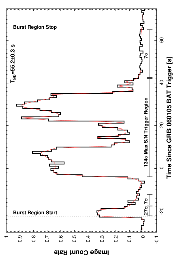
We employ the following automated 3-step procedure to define an optimum burst interval in the sense that it is likely to contain most of the source counts. An example event is shown in Figure 1 (Top Panel).

1. For every possible source extraction window t1–t2, by examining the cumulative distribution of detected counts in a light curve with 10ms bins, we record each interval of duration $\Delta t$ [s] with signal-to-noise ratio $S/N$ over threshold $S/N_{\rm min}={\rm MIN}(\sqrt{\Delta t},5)$. This trigger threshold suppresses the detection of entire emission episodes lasting longer than 25s. This is to avoid contamination due to count rate fluctuations that sometimes occur at the start or end of data acquisition due to the spacecraft slew. Low $S/N$ and long emission episodes are still detected, provided they are comprised of shorter regions, because:

2. We sort the triggers and dump temporal overlaps with lower $S/N$. The burst region is defined as the interval containing all surviving intervals. For the example shown in Figure 1 (Top Panel), the algorithm recovers four temporally separate triggers over threshold.

3. We allow the endpoints of this region to extend slightly outward to allow for the presence of a low $S/N$ rise or tail. With binsize $0.01~{}dt_{S/N}$, where $dt_{S/N}$ is the duration of the time window containing the maximal $S/N$ detection, we form a binned light curve and denoise the binned light curve with Haar wavelets (e.g., Kolaczyk & Dixon, 2000). The start (or end) of the initial burst region is allowed to extend by one additional bin for a total extension of $n_{\rm extend}$ bins as long as the $S/N$ of the denoised lightcurve in that bin is $>0.1~{}\sqrt{n_{\rm extend}}$, where 0.1 is the typical root-mean-square background noise fluctuation after denoising.

This final region is fixed and used for the timing and spectral analyses discussed below. In three cases (GRBs 060218, 061027, and 070126), the above procedure fails to detect a trigger and we must decrease the threshold in step 1 to $S/N_{\rm min}=3$.

2.2. Burst Duration Estimates

Using the burst intervals defined above for each event, we form the cumulative distribution of source counts and record the time values according to when a fraction 5, 25, 75, and 95% of the total counts arrive relative to the start of the burst interval. The difference between the 75 and 25 percentile time defines the burst $T_{50}$ duration, while the difference between the 95 and 5 percentile time defines the burst $T_{90}$ duration. We also determine a measure of duration $T_{r45}$ according to the prescription of Reichart et al. (2001). We also report the ratio of the peak rate Rate_p (in a time bin of width $0.01~{}dt_{S/N}$) over the total source counts (Cts). This is used to below to approximately relate the burst fluences reported in Table 2 to peak fluxes. We determine errors on each measured duration by performing a bootstrap Monte Carlo (e.g., Lupton, 1993), using the observed Poisson errors on the observed count rate. These duration values as well as the time region and $S/N$ ratio of the highest $S/N$ trigger for each burst are given in Table 1.

$T_{90}$ durations are strongly dependent on the choice of burst start and stop times, which are typically set by hand (e.g., Paciesas et al., 1999). We note the following loose consistency with the $T_{90}$ values reported by the Swift team without uncertainties on their public webage. Less than half (39%) of our $T_{90}$ values are consistent (1-sigma level) with those reported on the Swift webpage, assuming a 10% error for the Swift Team values. At the 3-sigma level, the consistency is 67%. Although individual values are inconsistent, it is important to note that we cannot reject the hypothesis that our $T_{90}$ distribution (see, also, Curtis et al., 2007) is consistent with that of the Swift Team (Kolmogorov-Smirnov (KS) test $P_{\rm KS}=0.7$).

2.3. Caveats, Manual Burst Region Edits

We separate short and long durations GRBs (e.g., Kouveliotou et al., 1993) here using a cutoff duration $T_{90}<3$s. The details of how our durations change with energy band and redshift are discussed in Curtis et al. (2007). In some cases, our automated algorithm detects a faint and long tail following some short GRBs. For GRB 050724, for example, there is a broad ($dt=20.7$ s) and late bump at 74 s after the main pulse ($dt=0.54$ s, $S/N=20.8$). For GRB 061006, the automated region selection above finds a broad $\approx 60$ s (see, also, Krimm et al., 2006) burst region due to a broad pulse with $S/N=14.7$. This lies under and after a narrow pulse of $S/N=42.6$ and $dt=0.82$ s. The ratio of the durations of these pulses ($\approx 40$ and 70, respectively) are $\mathrel{\hbox{\hbox to0.0pt{\hbox{\lower 4.0pt\hbox{$\sim$}}\hss}\hbox{$>$}}}3\sigma$ outliers with respect to the ratios found for all other BAT events. For this reason, we present in Table 2 spectral fits for both the full burst region and for the narrow pulse. We do this also for GRB 051227. We also conservatively label these events as “short-duration” events for exclusion in the analyses in Section 4.

The portion of of GRB 060124 which we analyze is only the pre-cursor to a much longer event (see, e.g., Romano et al., 2006b). The precursor is a factor $\approx 15$ fainter than the large flare which occurs $\approx 500$s later and for which only a light curve data are available.

Similarly we do not analyze the flux contribution to the unusual GRB 060218 (e.g., Campana et al., 2006a) after $t\approx 300$s.

2.4. Experimental Determination of the Detector Threshold

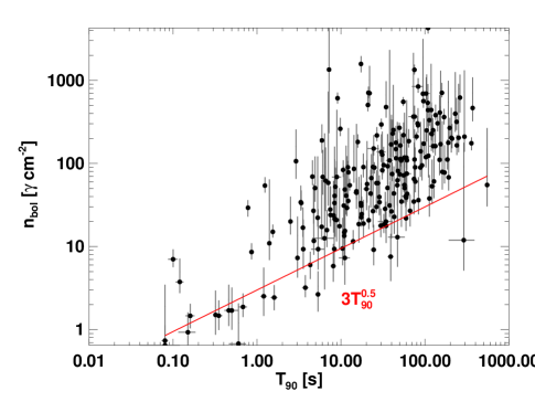
Plotting various observed quantities derived from the BAT spectra and light curves, we notice a strong correlation between the photon fluence and duration (e.g., Figure 2, Top Right). This correlation has also been noted by Berger (2007) for energy fluence in the case of short-duration GRBs only. Lee, Bloom, & Petrosian (2000) discuss a similar correlation found for pulses in BATSE bursts, which is unlikely to be due to cosmological effects.

The fluence and duration in the Swift sample are best fit by a powerlaw with index consistent with one half, which is suggestive of a detector threshold at the Poisson level. It is reasonable that the BAT detector could perform at or near the Poisson level over a wide range of burst durations due to the detector’s capacity to trigger on images (demasked light curves). A precise determination of the threshold, which is beyond the scope of this work, would involve modelling the satellite triggering algorithm and observational efficiency and also accounting for the sensitivity by the detector at different field angles for incident photons distributed in energy according to the true burst spectrum. We are interested here in obtaining an approximation to this threshold in terms of our best-fit values for detector independent quantities.

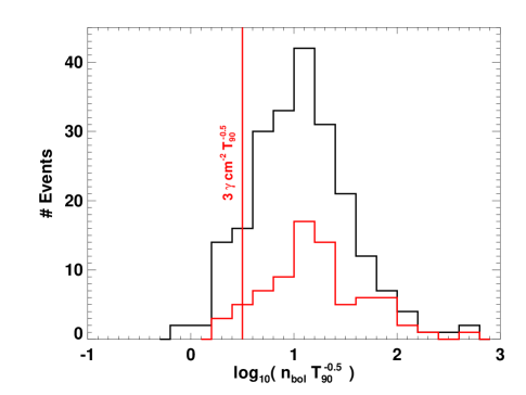
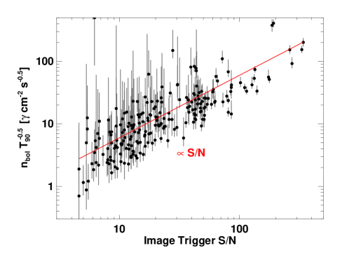
The fluence–duration correlation is likely due in part to the both shape of the typical GRB spectrum and also due to an intrinsic decrease in the number of bright relative to faint events. To test whether a truncation of the lowest fluence values by the detector threshold also contributes to the correlation, we plot the histogram of photon fluence over the square root of the $T_{90}$ duration (Figure 2, Top Left). There is a narrow clustering of values, and we find that $>90$% of events have $n_{\rm bol}/\sqrt{T_{90}}>3$ ph cm^-2 s^-0.5. Also, characteristic of a threshold, the observed $S/N$ of the maximal $S/N$ image trigger correlates tightly and linearly with $n_{\rm bol}/\sqrt{T_{90}}$ (Figure 2, Bottom Left). This clustering does not tighten if we consider a threshold in terms of peak photon rate instead of fluence over root time, as is typically the case for GRBs which fade rapidly in time (e.g., Band, 2003).

We find that the threshold in $n_{\rm bol}/\sqrt{T_{90}}$ corresponds to an $\approx 5\sigma$ detection threshold. The scatter around this best fit log-log line is $\sigma=0.52\pm 0.05$, determined using equation (14). Hence, the threshold estimator traces the actual threshold (as proxied by the observed $S/N$) to $\approx 50$% accuracy. There is no significant decrease in the scatter in Figure 2 (Bottom Left) or significant increase in the tightness of the histogram in Figure 2 (Top Left) if we attempt to include $E_{\rm pk,obs}$ (to some power) in the threshold estimate. We note that our value of $(n_{\rm bol}/\sqrt{T_{90}})_{\rm thresh}$ is closely consistent with the value estimated prior to Swift of $\approx 1$ ph cm^-2 s^-1 peak rate (1-$10^{3}$ keV) by Band (2003), after accounting for a slight increase due to a typical $\sqrt{T_{90}}\approx 3$ s^0.5. The Band (2003) threshold is also nearly independent of $E_{\rm pk,obs}$.

3. Spectral Fitting

We employ in parallel two spectral modelling approaches. The first is a classical frequentist approach that will be familiar to experienced users of the software package XSPEC (Arnaud, 1996). As we describe in the next subsection, we fit the data with the simplest of three possible models. We then derive confidence intervals by considering random realizations of the data given the best-fit model for each model parameter constrained by the best-fit model. This approach turns out to be very limited for Swift events, due to the narrow energy bandpass of the BAT instrument. In particular it is possible to measure a $\nu F_{\nu}$ spectral peak energy $E_{\rm pk,obs}$ for only about one third of the events in the sample. A more powerful Bayesian approach assumes that the each burst spectrum has an intrinsic spectrum containing the interesting $E_{\rm pk,obs}$ parameter, and we derive the probability distribution for that parameter given the data. We show below that prior information can be exploited to derive limits on $E_{\rm pk,obs}$ (and the burst fluence) even for cases where $E_{\rm pk,obs}$ is well above the detection passband.

3.1. Model Fitting 1: Frequentist Approach

We fit the time-integrated BAT spectra in the 15-150 keV band by forward folding an incident photon spectrum through the detector response. The resulting counts model is called $m(\vec{\theta})$ and is a function of the parameters $\vec{\theta}$. We find the best-fit model by minimizing:

$$\chi^{2}=\sum_{i}(y_{i}-m_{i}(\vec{\theta}))^{2}/\sigma_{i}^{2},$$ (1)

where $y_{i}$ is the count rate per energy in energy $E$ bin $i$ and $\sigma_{i}$ is the uncertainty (estimated from the source and background data) in $y_{i}$. To avoid falling into local $\chi^{2}$ minima, all minimization is done using a downhill simplex algorithm (e.g., Press et al., 1992) instead of the default XSPEC Marquardt algorithm (Arnaud, 1996).

We consider three possible models of increasing complexity to fit the time-integrated BAT spectra. These are a simple powerlaw, a powerlaw times an exponential cutoff, and a smoothly-connected broken powerlaw. The final model is the GRB Model (GRBM) of Band et al. (1993). We force this model to have a peak in the $\nu F_{\nu}$ spectrum in $E\in(0,\infty)$ by requiring that the low energy photon index $\alpha>-2$ and the high-energy photon index $\beta<-2$. Identifying the exponential times powerlaw model with the low energy portion of the GRBM spectrum, we require that the photon index for this model also satisfy $\alpha>-2$.

As we step from one model to the next, we add one additional parameter to the fit. Because the models are nested, the improvement in $\chi^{2}$ with each new parameter is distributed approximately as $\chi^{2}_{\nu}$ with $\nu=1$ degrees of freedom (e.g., Protassov et al., 2002). We only allow the step to a more complex model if the change in $\chi^{2}$ corresponds to a $>$90% confidence improvement in the fit. Errors on the parameters $\vec{\theta}$ are reported in Table 2 and are found from $\chi^{2}_{\rm min}$ in the vicinity of the global minimum as described in, e.g., Cash (1976).

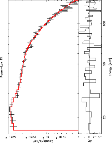
The middle panel of Figure 1 shows an example spectrum which is well fit by a powerlaw. All BAT bursts are adequately fit by one of the three models (Table 2).

In the 63% of cases where the data are adequately fit by a simple powerlaw model only, we also calculate a limit on $E^{\rm freq.}_{\rm pk,obs}$ as follows. If the photon index is more negative than $-2$ at 90% confidence, we use the constrained Band formalism (Sakamoto et al., 2004) to derive an $E^{\rm freq.}_{\rm pk,obs}$ upper limit. If the photon index is greater than $-2$ at 90% confidence, we derive an $E^{\rm freq.}_{\rm pk,obs}$ lower limit by fitting an exponential times powerlaw model. We warn the reader that lower and upper limits, respectively, on $E^{\rm freq.}_{\rm pk,obs}$ are undefined in these cases. Also, the probabilities associated with all quantities become poorly defined if the best-fit models have $\beta\approx-2$ or $\alpha\approx-2$, due the discontinuity in $\chi^{2}$ at these values (see, e.g., Protassov et al., 2002).

3.2. Model Fitting 2: Bayesian Approach

In the discussion below, we will be primarily interested in determining burst energetics via $E_{\rm pk,obs}$ and the bolometric GRB energy fluence. Because these quantities are poorly defined (if at all) for many BAT events in the frequentist approach, we consider also a more powerful Bayesian approach. The likelihood of the model given the data is

$$P(\vec{Y}|\vec{\theta})\propto\exp{(-\chi^{2}/2)}$$ (2)

From Bayes rule (e.g., Gregory, 2005) the posterior distribution gives the probability of the model, given the data

$$P(\vec{\theta}|\vec{Y})\propto P(\vec{Y}|\vec{\theta})P(\vec{\theta}),$$ (3)

where $P(\vec{\theta})$ in the prior probability on the model. We assume below that the prior can be broken into four multiplicative terms, one for each of the GRBM parameters. The posterior probability distribution for a given parameter $\theta_{i}$ is found by marginalizing $P(\vec{\theta}|\vec{Y})$ over the other parameters.

The power in the Bayesian approach comes from its capacity to allow us to incorporate pre-Swift knowledge of GRB spectra into our model fitting through the prior. Observations of thousands of GRBs by BATSE (e.g., Preece et al., 2000) strongly limit the range of likely GRBM parameters.

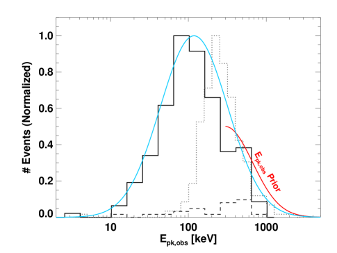
Most importantly (for Swift), the BATSE distribution in $E_{\rm pk,obs}$ falls off sharply above 300 keV (Preece et al., 2000; Kaneko et al., 2006). This leads us to the following prior on $ln[E_{\rm pk,obs}]$, ignoring the normalization:

$$P(ln[E_{\rm pk,obs}])\propto\exp{\left\{-0.5\left[ln\left({E_{\rm pk,obs}\over 300~{}{\rm keV}}\right)\right]^{2}/\sigma^{2}_{lE_{p}}\right\}},$$ (4)

for $E_{\rm pk,obs}>300$ keV, with $\sigma_{lE_{p}}=4/5$. We assume a uniform distribution in $ln[E_{\rm pk,obs}]$ below 300 keV instead of the cutoff observed by BATSE due to the high-energy bandpass of that instrument and to the discovery of X-ray Flashes (XRFs; Heise et al., 2000) which extends the distribution to low $E_{\rm pk,obs}$. We assign zero probability to $E_{\rm pk,obs}<1$ keV and $E_{\rm pk,obs}>10^{4}$ keV.

Kippen et al. (2002) (also, Barraud et al., 2003) show that the photon indices for XRFs are consistent with those found for GRBs. We assume the low energy powerlaw index distribution from BATSE (e.g., Kaneko et al., 2006):

$$P(\alpha)\propto\exp{(-0.5(\alpha-\alpha_{\rm pk})^{2}/\sigma^{2}_{\alpha})},$$ (5)

with $\alpha_{\rm pk}=-1.1$ and $\sigma_{\alpha}=0.25$.

There is evidence that the high-energy index distribution broadens with the inclusion of XRFs (see, Sakamoto et al., 2005). To be conservative, we assume only the peak of the BATSE distribution $\beta_{\rm pk}=-2.3$. We use the maximum entropy (e.g., Gregory, 2005) prior for a distribution of known mean:

$$P(\beta)\propto\exp{(-\beta/\beta_{\rm pk})}.$$ (6)

Finally, we assign equal probability per logarithmic interval to the model normalization, taken to be the fluence in the $1-10^{4}$ keV band (host frame, or source frame if redshift unknown) (see, also, Amati et al., 2002). We truncate this prior below $10^{-10}$ erg cm^-2 so that the integral over the model normalization remains finite. The specific value of this truncation is unimportant. We find identical results if we truncate instead at $10^{-50}$ erg cm^-2.

3.3. Most Probable Values, Samples, and Confidence Intervals

We find that the $E_{\rm pk,obs}$ marginal posterior probability distributions are typically broad and asymmetrical. We calculate these distributions explicitly for each event by integrating $P(\vec{\theta}|\vec{Y})$ analytically over model normalization and numerically over $\alpha$ and $\beta$. The 2-dimensional numerical integration is done via 10-point Gaussian quadrature (Press et al., 1992). At each step, we fit for and concentrate the integration in the region of maximal $P(\vec{\theta}|\vec{Y})$.

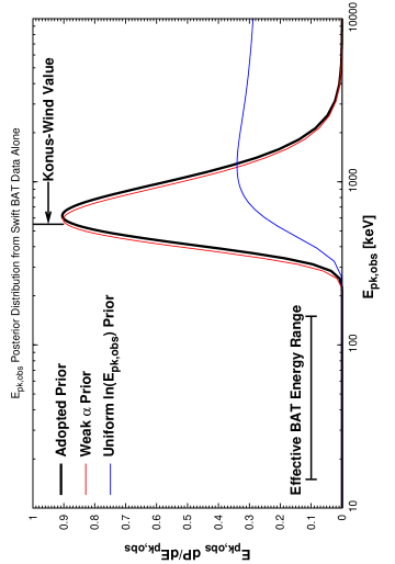
An example posterior probability curve is plotted in the bottom panel of Figure 1. With the adopted prior above, we recover an $E_{\rm pk,obs}$ value which is well above the Swift BAT bandpass and also consistent with Konus-Wind measurements (Golenetskii et al., 2006) in the 20–$2\times 10^{4}$ keV band.

Figure 1 also shows how the $E_{\rm pk,obs}$ determination changes as we relax our priors. Quadrupling the dispersion $\sigma_{\alpha}$ in the $\alpha$ prior has little effect at these high energies. However, if we discard the prior on $ln[E_{\rm pk,obs}]$ above 300 keV, then we are only able to derive a lower limit on $E_{\rm pk,obs}$ as in the frequentist approach ($E_{\rm pk,obs}>390$ keV; Table 2). At low energies, and analogous to the constrained Band formalism (Sakamoto et al., 2004), the prior on $\alpha$ helps to break the degeneracy between fitting a powerlaw spectrum associated with either the low-energy or the high-energy portion of the GRBM.

To describe the joint posterior probability distribution in $E_{\rm pk,obs}$ and fluence $E_{\rm iso}$, we obtain $10^{3}$ samples via a Markov Chain Monte Carlo (MCMC) simulation. We first draw $10^{3}$ samples from the marginal $E_{\rm pk,obs}$ posterior distribution (tabulated as discussed above). For each $E_{\rm pk,obs}$, we determine the mode of P($E_{\rm iso}$,$E_{\rm pk,obs}|\vec{Y}$) and the curvature at the mode. These define a Gaussian sampling distribution from which we take five Metropolis-Hastings steps (e.g., Gregory, 2005) in a random walk. The last $E_{\rm iso}$ value is saved, and the process is repeated $10^{3}$ times to store $10^{3}$ $E_{\rm pk,obs}$–$E_{\rm iso}$ pairs. Samples from the posterior distributions for each GRB with measured redshift are plotted in Figure 6. We use the $E_{\rm pk,obs}$ and $E_{\rm iso}$ samples to report the most probable values and intervals containing 90% of the posterior probability for all 218 bursts in Table 2.

3.4. $E_{\rm pk,obs}$ Constraints for Powerlaw Events

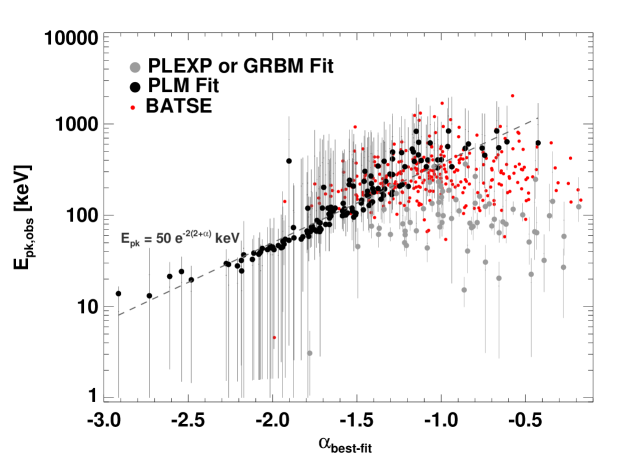
The referee has noted that our most-probable $E_{\rm pk,obs}$ values for events adequately fit by simple powerlaws correlate tightly with the best fit powerlaw indices $\alpha_{\rm best-fit}$ (Figure 3; also, Sakamoto et al., 2006). Indeed, because we wish to measure $E_{\rm pk,obs}$ from data which only constrain $\alpha_{\rm best-fit}$, this had better be the case. How does the correlation arise?

Half of the events, or about 30% of the total sample, produce the tightest region of the correlation and have $\alpha_{\rm best-fit}<-1.6$. Given our prior on the GRBM $\alpha$, these $\alpha_{\rm best-fit}$ are $2\sigma$ unlikely to be associated with the low energy index. Instead, the most-probable model steepens the index by placing $E_{\rm pk,obs}$ just above, in, and then below the BAT bandpass (see, also, Cabrera et al., 2007). We should not, therefore, interpret $\alpha_{\rm best-fit}$ as the GRBM $\alpha$ in this regime. However, we can also be confident that the data are strongly influencing $E_{\rm pk,obs}$.

The remaining half of events have $\alpha_{\rm best-fit}$ which could be associated with the GRBM $\alpha$. Above 200 keV, the steepening of $\alpha_{\rm best-fit}$ relative to $\alpha$ is comparable to the breadth of the $E_{\rm pk,obs}$ prior, and this makes the prior on $\alpha$ relatively unimportant in this regime (e.g., Figure 1, Bottom Panel). Because the exponential cutoff in the GRBM $E_{\circ}=(2+\alpha)E_{\rm pk,obs}$, the hardest events will still be most sensitive to low $E_{\rm pk,obs}$ values and will lead to tighter lower limits than for the softer events. The prior on $E_{\rm pk,obs}$ truncates the probability at high $E_{\rm pk,obs}$, and we continue to see a correlation, although with more scatter. Figure 3 shows how the $E_{\rm pk,obs}$ upper limits effectively account for possible large $E_{\rm pk,obs}$ values in the BATSE sample.

The average $E_{\rm pk,obs}$ for a large number of events in the regime $\alpha_{\rm best-fit}>-1.6$ is expected, therefore, to be unbiased with respect to BATSE GRBs with $E_{\rm pk,obs}>200$ keV. Also, the uncertainty in our estimate should account for the population $E_{\rm pk,obs}$ variations at high $E_{\rm pk,obs}$. Therefore, our $E_{\rm pk,obs}$ should still be useful for population studies (e.g., Sections 4.1,4.5). Our error regions are also likely to contain the true $E_{\rm pk,obs}$ for a given event.

Whether the most likely $E_{\rm pk,obs}$ for an individual burst closely corresponds to the true $E_{\rm pk,obs}$ will depend on whether or not $\alpha$ tends to be shallow for high $E_{\rm pk,obs}$. There is a weak but signifcant correlation ($\tau_{K}=0.18$, $5.1\sigma$) in GRBM fits to the Kaneko et al. (2006) BATSE sample, which indicates that this may be the case for some events. Contemporaneous measurement at energies above the BAT bandpass provide a direct test.

3.5. Comparison to Konus-Wind and Suzaku Measurements

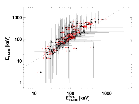
For 75 events in Table 2, we are able to determine lower and upper 90% confidence intervals for $E_{\rm pk,obs}$ using the classical frequentist approach (Figure 5; Top Left). The sample mean is $E^{\rm freq.}_{\rm pk,obs}=(79\pm 6)$ keV. We find consistent and unbiased $E_{\rm pk,obs}$ estimates from the Bayesian approach ($E_{\rm pk,obs}=(83\pm 6)$ keV). There is no strong evidence that the distributions are inconsistent ($P_{\rm KS}=0.88$). How does the Bayesian approach fare at higher energies where the spectra are typically acceptably modelled by powerlaws?

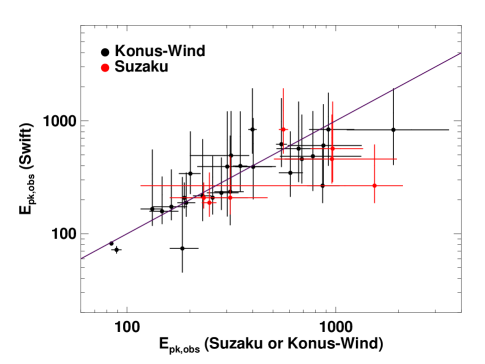
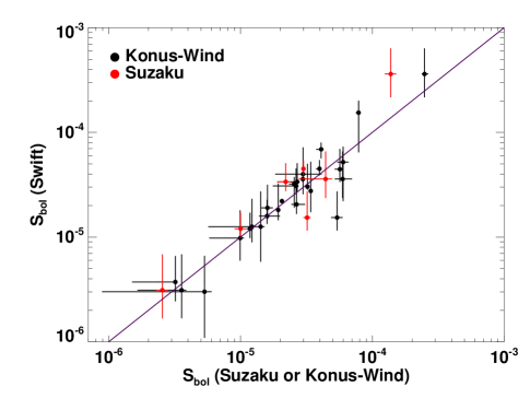
Comparing our Swift numbers to values from 27 observations by Konus-Wind reported in the Gamma-ray bursts Coordinates Network (GCN) circulars (e.g., Golenetskii et al., 2006), we find no evidence for bias in either our $E_{\rm pk,obs}$ or our $S_{\rm bol}$ determination (Figure 4). The sample means for both quantities are consistent at the $<1\sigma$ level ($\log_{10}{(S_{\rm bol,KW})}=-4.62\pm 0.08$ versus $\log_{10}{(S_{\rm bol,Sw})}=-4.62\pm 0.09$ and $\log_{10}{(E_{\rm pk,obs,KW})}=2.52\pm 0.06$ versus $\log_{10}{(E_{\rm pk,obs,Sw})}=2.47\pm 0.06$). There is no evidence from a KS-test ($P_{\rm KS}=$1.0, 0.9, for the fluence and $E_{\rm pk,obs}$ comparisons, respectively) that the distributions are different. Additionally, we note that there are very few discrepancies. We find that $>85$% of either our $E_{\rm pk,obs}$ values or our $S_{\rm bol}$ values are consistent within our estimated 90% confidence errors.

This agreement is remarkable considering that the Konus-Wind spectral fits are only the preliminary fits reported to the GCN. For seven of the events, Suzaku measurements are also reported in the GCN (e.g., Hong et al., 2007). We find no evidence for bias when comparing our Swift values instead to these (Figure 4).

To check that we are measuring $E_{\rm pk,obs}$ values above the BAT bandpass rather than simply assigning these all the same $E_{\rm pk,obs}$, we fit a powerlaw to the Swift and Konus-Wind data in Figure 4 (Left). To be conservative, we exclude the 8 points below 200 keV. For most (15 of 19) of these events, the Swift data are adequately fit by a powerlaw, and only one event has $\alpha_{\rm best-fit}<-1.6$. The remaining 4 of 19 events have weakly constrained $E^{\rm freq.}_{\rm pk,obs}$ values. The joint $E_{\rm pk,obs}$ data are fit by a powerlaw with index ($0.6\pm 0.2$) greater than zero at $\approx 5\sigma$ confidence.

Although this indicates information content in our $E_{\rm pk,obs}$ values, an index less than unity indicates a tendency to underestimate $E_{\rm pk,obs}$ at high $E_{\rm pk,obs}$. Our prior appears to lead to underestimates of large $E_{\rm pk,obs}\mathrel{\hbox{\hbox to0.0pt{\hbox{\lower 4.0pt\hbox{$\sim$}}\hss}\hbox{$>$}}}2$ MeV by a factor $\mathrel{\hbox{\hbox to0.0pt{\hbox{\lower 4.0pt\hbox{$\sim$}}\hss}\hbox{$>$}}}2$. We note that our estimates remain consistent within errors, that $E_{\rm pk,obs}$ understimates will be conservative as regards the analyses below, and that such very high $E_{\rm pk,obs}$ events are rare in the BATSE sample.

3.6. Comparison to BATSE Measurements

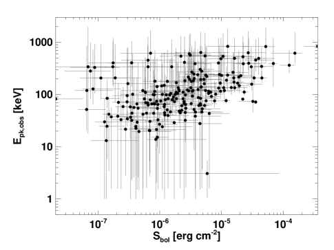
Figure 5 displays our fluence and $E_{\rm pk,obs}$ estimates. In the lower-right panel, an excess of low-$E_{\rm pk,obs}$ events is present relative to the $E_{\rm pk,obs}$ distributions determined by Kaneko et al. (2006) for bright BATSE GRBs. A similar effect is present in the HETE-2 catalog (Sakamoto et al., 2005). We also plot the best-fit Gaussian to the $E_{\rm pk,obs}$ data including errors (Section 4.1). There is marginal evidence for a shift in the peak of the $E_{\rm pk,obs}$ distribution. The prior we assume on $E_{\rm pk,obs}$ (from BATSE) is at least partially responsible for this effect. Further analyses and comparisons of our $E_{\rm iso}$ and $E_{\rm pk}$ estimates to those found for previous GRBs, also using our XRT analyses (Butler & Kocevski, 2007a, b), are presented in Kocevski et al. (2007).

4. Discussion

4.1. $E_{\rm iso}$–$E_{\rm pk}$ Correlation and Intrinsic Scatter

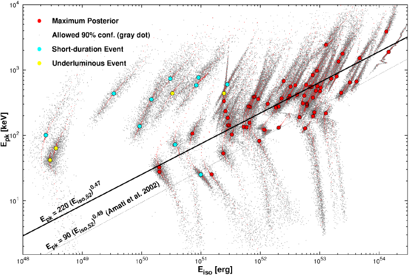
In this section, we use the $10^{3}$ pairs of $E_{\rm iso}$–$E_{\rm pk}$ samples accumulated above, which fully account for correlations between the GRBM parameters for each of 77 bursts with measured redshift, in order to test the well known burst-to-burst relation $E_{\rm pk}=(1+z)E_{\rm pk,obs}\approx K(E_{\rm iso}/[10^{52}{\rm~{}erg}])^{\eta}$ keV (e.g., Lloyd, Petrosian, & Mallozzi, 2000; Amati et al., 2002). The samples, aside from the most peripheral 10%, are plotted in Figure 6 along with the best fit powerlaw we derive below. These are publicly available from our webpage and should be used in place of the best-fit values (Table 2) when fitting models to the data. As we illustrate below, these samples can be used to rigorously determine the normalization, slope, and scatter, even when large measurement errors are present.

First it is interesting to know what fraction of the total number of events have at least $10^{2}$ samples on the opposite side of the best fit line of Amati et al. (2002, i.e. $K=90$, $\eta=0.49$) from the main mass of samples. This provides a measure of consistency at the 90% confidence level. To be conservative, we allow the Amati et al. (2002) relation to have a logarithmic dispersion of $\pm 0.7$ (i.e., 0.3 dex). We also toss out strong outliers from our sample. We ignore the short-duration and underluminous events marked in yellow and cyan in the Figure 6. We use an ad hoc (and admittedly circular) definition of underluminous: the $E_{\rm iso}$ is 100 or more times fainter than that expected from the Amati et al. (2002) relation, given the best-fit $E_{\rm pk}$. The underluminous events with long durations are GRBs 051109B, 060218, and 060614. After removing the underluminous and short duration events and retaining only those marked with red circles in Figure 6, we find that 41% ($26/63$) of Swift events are inconsistent with the Amati et al. (2002) powerlaw at the 90% confidence level.

We now determine the best $E_{\rm iso}$–$E_{\rm pk}$ powerlaw relation for the Swift data. For each event $j$, the $10^{3}$ samples represent the posterior probability $P(E_{j,{\rm iso}},E_{j{\rm pk}}|\vec{Y})$ (Section 3.2). Using the $(E_{\rm iso},E_{\rm pk})$ values corresponding to the posterior peak in each event (Table 2), there is evidence for a strong correlation (Section 4.4). What are the values of $K$ and $\eta$ describing this correlation via a powerlaw fit, and what is the true scatter around this fit?

For simplicity in notation we write $x_{j}=ln(E_{j,{\rm iso}}/[10^{52}{\rm~{}erg}])$ and $y_{j}=ln(E_{j,{\rm pk}})$. We now assume for each burst a prior between $x_{j}$ and $y_{j}$ representing a powerlaw relation between $E_{\rm iso}$ and $E_{\rm pk}$:

$$P(x_{j},y_{j}|k,\eta,\sigma_{A})\propto\\ \exp{(-0.5[y_{j}-k-\eta x_{j}]^{2}/\sigma^{2}_{A})}/\sigma_{A},$$ (7)

where $\sigma_{A}$ allows for an intrinsic scatter in the correlation. By inverting the data in this fashion to determine the intrinsic scatter (rather than just assuming that the observed scatter is the intrinsic scatter), we rigorously account for the large $E_{\rm pk,obs}$ uncertainties arising from the narrow BAT bandpass. The parameter $\sigma_{A}$ also plays an important role in allowing the powerlaw model to acceptably fit the data, as we discuss in Section 4.2.

Equation (7) multiplies the posterior $P(x_{j},y_{j}|\vec{Y})$ for each event to form the posterior probability of $k$, $\eta$, and $\sigma_{A}$ for that event. The posterior considering all $N$ events is then:

$$P(k,\eta,\sigma_{A},x_{j},y_{j}|\vec{Y})\propto~{}\sigma^{-N-1}_{A}\prod_{{\rm event}~{}j}P(x_{j},y_{j}|\vec{Y})\\ \times\exp{(-0.5[y_{j}-k-\eta x_{j}]^{2}/\sigma^{2}_{A})}.$$ (8)

Here we have included a $1/\sigma_{A}$ prior on $\sigma_{A}$ (i.e., equal probability per logarithmic interval or scale invariance). We assume uniform priors on $k$ and $\eta$. Because $P(x_{j},y_{j}|k,\eta,\sigma_{A})=P(y_{j}|x_{j},k,\eta,\sigma_{A})P(x_{j}|k,\eta,\sigma_{A})$, we are effectively setting a uniform prior on $x_{j}$ as well.

We wish now to marginalize over the $(x_{j},y_{j})$. This can be accomplished by Monte Carlo integration using the $10^{3}$ samples $i$ for each event:

$$P(k,\eta,\sigma_{A}|\vec{Y})\propto~{}\sigma^{-N-1}_{A}\\ \times\prod_{{\rm event}~{}j}\left\{\sum_{{\rm samp}~{}i~{}}\exp{(-0.5[y_{i,j}-k-\eta x_{i,j}]^{2}/\sigma^{2}_{A})}\right\},$$ (9)

where $x_{i,j}$ designates the $i$th sample of $x_{j}$. Because the $P(x_{j},y_{j}|\vec{Y})$ are independent, we can carry out the product before the sum in Equation 8, provided we randomize away any sorting that may have occurred in the tabulation of the $(x_{i,j},y_{i,j})$. Defining $\Theta_{i}\equiv\sum_{j}[y_{i,j}-k-\eta x_{i,j}]^{2}$, we have:

$$P(k,\eta,\sigma_{A}|\vec{Y})\propto~{}\sigma^{-N-1}_{A}\left\{\sum_{{\rm samp}~{}i~{}}\exp{(-0.5\Theta_{i}/\sigma^{2}_{A})}\right\}.$$ (10)

If we define the following statistics for the set of $i$th samples averaged over events $j$, $mx_{i}={<x_{i,j}>_{j}}$, $my_{i}={<y_{i,j}>_{j}}$ $vx_{i}={<x^{2}_{i,j}>_{j}-mx^{2}_{j}}$, $vy_{i}={<y^{2}_{i,j}>_{j}-my^{2}_{j}}$, $cov_{i}={<x_{i,j}y_{i,j}>_{j}}-mx_{j}my_{j}$, we can marginalize to find:

$$P(k,\eta|\vec{Y})\propto\sum_{{\rm samp}~{}i}[k^{2}+2k\eta~{}mx_{i}-2k~{}my_{i}+\\ \eta^{2}(vx_{i}+mx^{2}_{i})-2\eta(cov_{i}+my_{i}~{}mx_{i})+(vy_{i}+my^{2}_{i})]^{-N/2},$$ (11)

$$P(k|\vec{Y})\propto\sum_{{\rm samp}~{}i}(vx_{i}+mx_{i}^{2})^{(N-2)/2}\\ [(vy_{i}+my_{i}^{2})(vx_{i}+mx_{i}^{2})-(cov_{i}+mx_{i}my_{i})^{2}-\\ 2k(my_{i}~{}vx-mx_{i}~{}cov_{i})+k^{2}~{}vx_{i})]^{-(N-1)/2},$$ (12)

$$P(\eta|\vec{Y})\propto\sum_{{\rm samp}~{}i}(\eta^{2}~{}vx_{i}-2\eta~{}cov_{i}+vy_{i})^{-(N-1)/2},~{}{\rm and}$$ (13)

$$P(\sigma_{A}|\vec{Y})\propto\sigma^{-N+1}_{A}\\ \times\sum_{{\rm samp}~{}i}vx_{i}^{-1/2}\exp{(-0.5N[vy_{i}-cov_{i}^{2}/vx_{i}]/\sigma^{2}_{A})}.$$ (14)

In a similar fashion to the derivation of these formulae, it is interesting to know the intrinsic distribution of individual parameters if we assume that this distribution is a Gaussian, i.e.,

$$P(x_{j}|\vec{Y})\propto\exp{(-0.5[x_{j}-x_{\circ}]^{2}/\sigma^{2}_{\rm x})}/\sigma_{\rm x}.$$ (15)

As in Equation (11),

$$P(x_{\circ}|\vec{Y})\propto\sum_{{\rm samp}~{}i}[(x_{\circ}-mx_{i})^{2}+vx_{i}]^{-N/2}.$$ (16)

As in Equation (14),

$$P(\sigma_{\rm x}|\vec{Y})\propto~{}\sigma^{-N}_{\rm x}\sum_{{\rm samp}~{}i}\exp{(-0.5Nvx_{i}/\sigma^{2}_{\rm x})}.$$ (17)

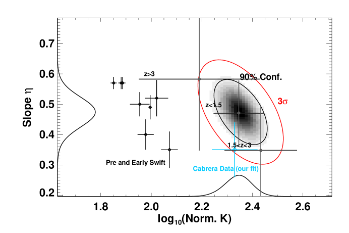
Figure 7 shows Equations (11, 12, and 13) for the 63 events marked by red circles in Figure 6. We find that the posterior (Equation 11) peaks at $\log_{10}{(K)}=2.35\pm 0.09$ and $\eta=0.47\pm 0.08$. This is inconsistent at the $>5\sigma$ level with all pre-Swift curves. There is also large intrinsic scatter in the relation $\sigma_{A}=0.7\pm 0.1$ ($0.30\pm 0.04$ dex), given the Swift data.

Comparatively, the observed scatter (Equation 14 for just the best fit $E_{\rm pk}$ and $E_{\rm iso}$ values; Table 2) is 0.46 dex. This latter value is an unfair estimate of the true scatter, because it is contaminated by the relatively weak $E_{\rm pk,obs}$ determinations (Figure 6) due to the narrow BAT bandpass. The intrinsic scatter we calculate is far larger than the pre-Swift estimate of $0.14^{+0.3}_{-0.2}$ dex by Amati et al. (2006). Because $\sigma_{A}$ refers to the scatter in the logarithm, our value corresponds to a factor of 2 intrinsic scatter in the powerlaw relation $E_{\rm pk}=KE_{\rm iso}^{\eta}$.

Li (2007) observes a possibly significant variation in $K$ and $\eta$ with redshift for the pre-Swift sample. For the Swift sample, we observe no significant evidence for such variations (Figure 7). Also, we note that possible variations appear to be non-monotonic. The intrinsic scatter does not vary significantly: $\sigma_{A}=0.58^{+0.20}_{-0.14}$ ($z<1.5$), $\sigma_{A}=0.53^{+0.24}_{-0.14}$ ($1.5<z<3.0$), and $\sigma_{A}=0.65^{+0.20}_{-0.16}$ ($z>3$).

There is little evidence for an $E_{\rm pk}$-$E_{\rm iso}$ relation in the Swift short-duration GRB sample, because the relation has large errors $\log_{10}{(K)}=2.7\pm 1.0$, $\eta=0.1^{+0.4}_{-0.5}$ and a large intrinsic scatter $\sigma_{A}=1.3^{+0.8}_{-0.5}$. Also, $\eta$ is consistent with zero.

4.2. Comparison with Cabrera et al. (2007)
$E_{\rm pk}$-$E_{\rm iso}$ Relation

As described above, Cabrera et al. (2007) measure $E_{\rm pk}$ and $E_{\rm iso}$ for 28 Swift GRBs with measured redshift — a subsample of the full 77 GRB sample considered here. They account for the detector-dependent correlation between these quantities for each GRB with a Gaussian approximation. We have retrieved their best fit $E_{\rm pk}$ and $E_{\rm iso}$ and confidence regions (their Table 3), drawn $10^{3}$ samples from the appropriate bivariate-Gaussian distributions for each event, and fit the data using Equations (12-14).

We find $\log_{10}{(K)}=2.33\pm 0.09$ and $\eta=0.35\pm 0.09$ (Figure 7), and an intrinsic scatter $\sigma_{A}=0.4\pm 0.1$ ($0.18\pm 0.04$ dex). These parameters are closely consistent with those that we derive above for our full sample, although $\sigma_{A}$ is larger for the full sample. We find identical maximum posterior values and confidence regions with the linmix_err MCMC regression tool (Kelly, 2007) in IDL, which sets different priors for the $E_{{\rm iso},j}$ and $\sigma_{A}$.

Because Cabrera et al. (2007) employ a Gaussian error approximation, a powerlaw fit to their $E_{\rm pk}$ and $E_{\rm iso}$ values can also be obtained from a simple $\chi^{2}$ minimization procedure. Following Press et al. (1992), we minimize

$$\chi_{p}^{2}=\sum_{i}{(y_{i}-k-\eta x_{i})^{2}\over(\sigma^{2}_{y_{i}}+\eta^{2}\sigma^{2}_{x_{i}}-2\rho_{i}\eta\sigma_{x_{i}}\sigma_{y_{i}}+\sigma_{A}^{2})},$$ (18)

where $\sigma_{x_{i}}$ and $\sigma_{y_{i}}$ are the errors on $x_{i}$ and $y_{i}$, respectively, and $\rho_{i}$ is the Pearson correlation coefficient between $x_{i}$ and $y_{i}$ (labeled “cov” in Table 3 of Cabrera et al. (2007)). Fixing $\sigma_{A}=0.4$ and minimizing $\chi^{2}_{p}$, we find $\log_{10}{(K)}=2.32\pm 0.08$ and $\eta=0.32\pm 0.19$, for $\chi^{2}_{p}/\nu=21.9/26$. This is consistent with our Monte Carlo fits above but inconsistent with the Monte Carlo fit reported in Cabrera et al. (2007): $\log_{10}{(K)}=2.03\pm 0.01$ and $\eta=0.53\pm 0.03$.

For $\sigma_{A}=0$, the Cabrera et al. (2007) fit has $\chi^{2}_{p}/\nu=445.7/26$. It is clear from Figures 4 and 5 in Cabrera et al. (2007) that their fit does not match the data well and that the fit errors are under-estimated. The quoted errors are under-estimated by at least a factor $(\chi^{2}_{p}/\nu)^{0.5}\approx 4$.

It is not entirely clear how such a poorly-fitting model was chosen by those authors. It is likely that assuming $\sigma_{A}=0$ precludes finding a statistically acceptable model: our best-fit model with $\sigma_{A}=0$ has $\log_{10}{(K)}=2.11$ and $\eta=0.23$ ($\chi^{2}_{p}/\nu=366.4/26$).

4.3. Differences Between the Amati et al. (2002) Consistent and Outlier Samples

Separating the 59% of events above found to be consistent with the Amati et al. (2002) relation at 90% confidence from those found to be inconsistent, we perform a number of 2-sample KS tests on the observables in Tables 1 and 2. We adopt a functional definition of inconsistency between these sub-samples: the KS test NULL hypothesis probability that the sub-samples are drawn from the same parent distribution is $P_{\rm KS}<0.01$. We find that the sub-sample distributions goodness of fit $\chi^{2}/\nu$, $T_{90}$ duration, and fluence are all consistent. The redshift and $E_{\rm iso}$ distributions are also consistent. Contrarily, the photon fluences are lower on average by a factor $\approx 2.3$ ($P_{\rm KS}=9.8\times 10^{-3}$) in the observer frame and $\approx 2.7$ in the source frame ($P_{\rm KS}=1.4\times 10^{-3}$). Because the energy fluences were consistent, we expect and observe that the Amati et al. (2002) inconsistent events are on average a factor $\approx 2.5$ times harder ($P_{\rm KS}=4.1\times 10^{-4}$) in terms of $E_{\rm pk,obs}$, or a factor $\approx 1.5$ in $E_{\rm pk}$ ($P_{\rm KS}=9.3\times 10^{-3}$).

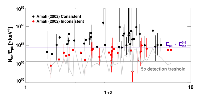
The differences in $N_{\rm iso}$ and $E_{\rm pk}$ between the two samples are most apparent when we plot the ratio of these quantities (Figure 8). Because $E_{\rm iso}\propto E_{\rm pk}N_{\rm iso}$ (e.g., Figure 5, Bottom Left), a powerlaw relation $E_{\rm peak}\propto E^{0.5}_{\rm iso}$ like that found above for the full Swift sample and by Amati et al. (2002) for GRBs observed by Beppo-SAX translates to a line of constant $N_{\rm iso}/E_{\rm pk}$. We also plot the observed $5\sigma$ detection threshold, determined by scaling the observed $N_{\rm iso}/E_{\rm pk}$ by $5/(S/N)$. As we discuss in more detail in the next section, a dividing line between events detected by a satellite of greater sensitivity (Swift versus Beppo-SAX) points to a detector threshold selection effect.

To be quantitative, we perform the following bootstrap simulation which approximately conserves the local fraction of events per energy flux interval. In redshift steps $dz=1$, we shuffle the observed $E_{\rm peak}$, $T_{90}$, and $z$ values and calculate $N_{\rm iso,new}=N_{\rm iso}(E_{\rm pk}/E_{\rm pk,new})/(T_{90,{\rm new}}/T_{90})$ for each event several times. We observe that no simulated events above the horizontal line drawn in Figure 8 are lost due to a threshold in $N_{\rm iso}/\sqrt{T_{90}}$ (Section 2.4). However, 30% of events below the line fall below threshold. If we increase the Swift threshold by a factor of 3 (see, Band, 2003) to obtain an approximate Beppo-SAX threshold, then 65% percent of events below the line are lost, while only 2% are lost above the line. If we increase the Swift threshold by a factor of 10 — as is suggested by the Firmani et al. (2006) relation (Section 4.6) — then nearly all (96%) of events below the line are lost while only 34% are lost above the line.

An alternative explanation for why our $E_{\rm pk}$–$E_{\rm iso}$ relation is inconsistent with the pre-Swift relations is that the Swift GRBs are intrinsically different from pre-Swift GRBs. Most must have $E_{\rm pk}$ values which are $(2.5)^{2}\approx 6$ times harder on average, assuming that they have similar photon fluences. We are very confident that our analysis — which determines $E_{\rm pk,obs}$ for an approximately fixed photon fluence — could not yield an error this large for individual events and certainly not for a large number of events.

Our prior assumptions cannot be the dominant source of inconsistency. A similar fraction ($\approx 60$%) of events for both the Amati et al. (2002) consistent and inconsistent classes are adequately fit by powerlaws, and the number of events in each class with $\alpha_{\rm best-fit}<-1.6$ (see Section 3.4) are comparable. Moreover, if some events adequately fit by a simple powerlaw in the classical frequentist approach actually did have extremely high $E_{\rm pk}\mathrel{\hbox{\hbox to0.0pt{\hbox{\lower 4.0pt\hbox{$\sim$}}\hss}\hbox{$>$}}}1$ MeV, these would be underestimated given our prior, and the actual values would be more inconsistent with the pre-Swift relations.

Also, the priors can be discarded, and similar results are found. Our best-fit $E_{\rm pk}$ and $E_{\rm iso}$ values (Table 2) for the events shared between our and the Cabrera et al. (2007) analyses are closely consistent. The fits lead to a closely consistent $E_{\rm pk}=KE_{\rm iso}^{\eta}$ relation (Section 4.2). If we retain our priors but replace our Swift numbers with the 7 closely-consistent $E_{\rm pk,obs}$–$E_{\rm iso}$ pairs available from the Konus-Wind sample (Section 3.5) of GRBs with measured redshifts, we also find statistically indistinguishable results.

The difference in the Swift sample cannot be a difference due to the higher redshifts, because the low-$z$ events in the Swift sample dominate the relation and force it to be inconsistent with the pre-Swift relation (Figure 7). The high-$z$ events produce the most consistent $E_{\rm pk}$–$E_{\rm iso}$ relation to that of Amati et al. (2002).

4.4. The $E_{\rm pk}$–$E_{\rm iso}$ Correlation as a Threshold Effect

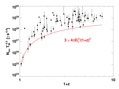
It is apparent from Figure 2 (Bottom Right) that the BAT detector threshold leads to a strong truncation of detected events with redshift. We show above how this truncation can help to narrow the scatter in a powerlaw $E_{\rm pk}$–$E_{\rm iso}$ relation, making that relation more consistent with a pre-Swift relation found by Amati et al. (2002). Our observed relation corresponds to fainter and harder events, in agreement with indications from spectral fits to BATSE GRBs (Nakar & Piran, 2005; Band & Preece, 2005) that the relation may in fact be an inequality.

In agreement with previous studies (Amati et al., 2002; Amati, 2003; Ghirlanda, Ghisellini, & Lazzati, 2004; Friedman & Bloom, 2005; Nava et al., 2006; Amati et al., 2006), we find that $E_{\rm iso}$ and $E_{\rm pk}$ are tightly correlated (e.g., Figure 6). We find a Kendall’s $\tau_{K}=0.59$ ($6.8\sigma$ significant), for the best-fit values (Table 2) in 63 bursts.

A correlation between $E_{\rm pk}$ and $E_{\rm iso}$ could come about in two very different ways. First (1), there could be an intrinsic correlation between these quantities in the source frame, as is widely held (e.g., Cabrera et al., 2007). Alternatively (2), these quantities could be correlated in the observer frame (or just narrowly-distributed) and a strong correlation arises when we multiply both quantities by strong functions of redshift. The most straight-forward way to rule out (2) in favor of a true source frame correlation is to show that there is no strong correlation among values in the observer frame. If that fails, as it does for the Swift sample, we can argue against (2) by attempting to show that the source frame correlation represents a tighter clustering. The source frame clustering then presumably leads to the observer frame clustering. To demonstrate a significantly tighter clustering in the source frame, we must control for the increase in clustering which arises due to multiplication by factors containing redshift.

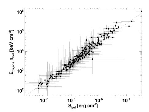
If we separate the terms in the $E_{\rm iso}$-$E_{\rm pk}$ powerlaw fit containing redshift from those not containing redshift (e.g., Nakar & Piran, 2005), we see that the redshift independent terms $\approx S^{0.5}_{\rm bol}/E_{\rm pk,obs}$ ($\approx\sqrt{n_{\rm bol}/E_{\rm pk,obs}}$) exhibit a narrow scatter of $0.32\pm 0.05$ dex. (There is a strong observer frame correlation between our best-fit $S_{\rm bol}$ and $E_{\rm pk,obs}$: $\tau_{K}=0.49$, $5.7\sigma$.) This is consistent with the scatter about the $E_{\rm iso}$-$E_{\rm pk}$ relation (Section 4). Stated differently, we can ignore the actual data and randomly sample the ratio $S_{\rm bol}/E_{\rm pk,obs}$ from a lognormal distribution and recover an equally significant (but fake) $1+z$ versus $E_{\rm iso}/E_{\rm pk}$ correlation in a majority (94%) of simulations. The narrow scatter in these observer frame quantities is likely a consequence of the detector threshold, because there is less scatter in $\sqrt{n_{\rm bol}}$ alone ($0.23\pm 0.04$ dex) and in $\sqrt{n_{\rm bol}/T^{0.5}_{90}}$ ($0.19\pm 0.03$ dex; Figure 2; Top Left). Moreover, the scatter in $\sqrt{n_{\rm bol}/T^{0.5}_{90}}$ ($0.24\pm 0.04$ dex) changes little if we also include the short-duration and underluminous events.

In addition to a weak dependence on the actual fluence and $E_{\rm pk,obs}$ data, little source frame information appears to be encoded in the $E_{\rm iso}$-$E_{\rm pk}$ correlation. If we shuffle the redshifts among the sample, drawing with repetition one redshift for each burst and recalculating the source frame quantities given the observer frame quantities, we find that a stronger correlation happens by chance in a large fraction (42%) of simulations. Schaeffer & Collazzi (2007) discuss in detail the redshift degeneracy in the $E_{\rm iso}$-$E_{\rm pk}$ and other high-energy relations.

We show now how the $E_{\rm iso}$-$E_{\rm pk}$ correlation can arise due to partial correlation with the detector threshold. First we divide the $E_{\rm iso}$, $E_{\rm pk}$ through by $E_{\rm pk,obs}$ and find that $(1+z)$ and $E_{\rm iso}/E_{\rm pk,obs}$ are tightly correlated ($\tau_{K}=0.53$, $6.2\sigma$ significance). The expected threshold for $E_{\rm iso}/E_{\rm pk,obs}$ scales as $D_{L}^{2}/(1+z)\sqrt{T_{90}}$. Controlling for partial correlation with this quantity (see, Akritas & Siebert, 1996), we find that the $E_{\rm pk}$-$E_{\rm iso}$ correlation has $\tau_{K,{\rm partial}}=0.12$, with a significance of only $1.5\sigma$. We conclude that the detector threshold accounts for a substantial portion of the $E_{\rm iso}$-$E_{\rm pk}$ correlation seen for Swift events.

Previous studies (e.g., Amati et al., 2002) have concluded that the $E_{\rm pk}$–$E_{\rm iso}$ correlation is not due to a flux selection effect because individual burst fluences tend to lie well above the detector threshold. This is not a strong enough argument, however, because even highly significant detections can be affected by a threshold bias if the values follow the threshold and are clustered (e.g., Figure 2; Top Left). We can then invent apparent source frame correlations of arbitrarily small significance (i.e., very significant) by multiplying by steeper and steeper function of redshift.

It is also argued that the large dynamic range in $E_{\rm pk,obs}$ and fluence over which the pre-Swift $E_{\rm pk}$–$E_{\rm iso}$ relation is observed makes it less likely to be a selection effect. However, the ratio of fluence to $E_{\rm pk,obs}$ is narrowly-distributed (i.e., these quantities are highly correlated in the observer frame; Figure 5, Top Right), even for the pre-Swift sample (see, e.g., Amati et al., 2002; Sakamoto et al., 2005), and this ratio is what we should require to exhibit a large dynamic range.

4.5. Other High-Energy Correlations

A number of correlations have been reported in the literature among GRB timing and spectral parameters in addition to the $E_{\rm iso}$–$E_{\rm pk}$ correlation. We can test three of these against the Swift data set in Tables 1 and 2.

Firmani et al. (2006) have performed a careful search over high-energy parameters in fits to 27 pre-Swift GRBs in order to find a very tight correlation $L_{\rm iso}\approx 10^{48.5\pm 0.1}(E_{\rm pk}^{1.62}T^{-0.49}_{z,r45})$. We find a consistent but less tightly constrained relation from the Swift sample: $L_{\rm iso}\approx 10^{48.5\pm 0.7}(E_{\rm pk}^{1.62}T^{-0.49}_{z,r45})^{0.86\pm 0.15}$. Here, the duration $T_{r45}$ (Tables 1 & 2) is transformed to the source frame according to the prescription in Firmani et al. (2006), $T_{z,r45}r=T_{r45}/(1+z)((1+z)/2)^{0.4}$, which accounts for the BAT energy range. The most-probable new relation has large intrinsic scatter of $0.58\pm 0.8$ dex.

The Firmani et al. (2006) relation broadens in the Swift sample due to the excess of hard and low-luminosity events. We find that most Swift events (60% or $38/63$) are inconsistent with the pre-Swift Firmani et al. (2006) relation at the 90% confidence level. Stated differently, most (71%) of the Swift GRB 90% confidence redshift intervals on a redshift estimator $\hat{z}$ determined assuming the relation do not contain the actual redshift.

Using Equation 17 to account for the large uncertainties in $\log_{10}{(1+\hat{z})}$, we find that there is a large intrinsic scatter of $0.6\pm 0.1$ dex between this and the same of function using the host galaxy/spectroscopic redshift. We find that 50% of the probability in terms of estimated redshift for 40% of events is at $z>10$, due to the faintness and hardness of the Swift events. Ignoring these cases, the 90% confidence redshift estimate still fails for 53% ($20/38$) of events. There is only a weak correlation ($\tau_{K}=0.17$, $1.9\sigma$) between the best-fit redshift assuming the relation and the actual redshift.

The Swift Firmani et al. (2006) correlation, using the best-fit parameters from Tables 1 & 2, has $\tau_{K}=0.61$ ($7.1\sigma$). However, this decreases to $\tau_{K,{\rm partial}}=0.13$ ($1.5\sigma$) if we control for partial correlation with the detector threshold. Because the ratio of source frame quantities used in the Firmani et al. (2006) relation is narrowly-distributed for the Swift sample (0.45 dex), we find that most simulations (71%) of the source frame correlation using fake observer frame data yield a more significant source frame correlation.

We observe a significant correlation between $L_{\rm iso}$ and $E_{\rm peak}$ (see, Schaeffer, 2003; Yonetoku et al., 2004), with $\tau_{K}=0.55$ ($6.3\sigma$) for our best-fit model parameters (Tables 1 & 2). However, if we control for partial correlation with the detector threshold as above, the correlation largely disappears ($\tau_{K,{\rm partial}}=0.15$, $\sigma=1.8$). Most simulations (96%) of the source frame correlation using fake observer frame data yield a more significant source frame correlation.

Atteia (2003) find a tight correlation between $N_{\rm iso}/E_{\rm pk,obs}/\sqrt{T_{90}}$ and $1+z$ for data detected by the HETE-2 satellite, which is used as a redshift estimator. We find a modestly significant correlation ($\tau_{K}=0.38$, $4.4\sigma$) among our best fit parameters (Tables 1 & 2). As hinted by the similar form of the Atteia (2003) redshift estimator to our $S/N$ estimator ($n_{\rm bol}/\sqrt{T_{90}}$; Section 2.4), the correlation strength degrades greatly when we control for partial correlation with the detector threshold ($\tau_{K,{\rm partial}}=0.14$, $1.6\sigma$). Most simulations ($>$99%) of the source frame correlation using fake observer frame data yield a more significant source frame correlation.

We note that the Atteia (2003) correlation and the correlations above can be used as redshift estimators only if one believes that the correlation exists in the source frame, independent of the observer frame detector threshold.

We do not test here the veracity of correlations between temporal lag and luminosity (e.g., Norris, Marani, & Bonnell, 2000) or temporal variability and luminosity (e.g., Fenimore & Ramirez-Ruiz, 2000). However, we stress that future analyses testing these correlations must account for the detector threshold.

We also do not test the correlation between $E_{\rm pk}$ and the beaming corrected energy release $E_{\gamma}$ found by (Ghirlanda, Ghisellini, & Lazzati, 2004) (see, also, Liang & Zhang, 2005). This requires measurement of late-time light curve breaks, and these appear to be ambiguous or non-existent for many Swift events (Sato et al., 2007; Willingale et al., 2007). Panaitescu (2007) find that the $E_{\rm pk}$-$E_{\gamma}$ exists in the Swift sample but is largely a consequence of the $E_{\rm pk}$-$E_{\rm iso}$ correlation. We explore this issue in a separate paper (Kocevski et al., 2007).

4.6. The pre-Swift Threshold and Low-$z$ Events

We assume here that the pre-Swift correlations represent measures of detection threshold. In addition to the instrument that detected the GRB (e.g., HETE-2 or Beppo-SAX), this includes biases due to the source localization, optical afterglow brightness and host galaxy brightness and star formation rate. There are also likely strong biases due to outlier rejection during the construction of the correlations. The Firmani et al. (2006) relation is potentially the best measure of the sum total of these biases, because that relation has the narrowest scatter.

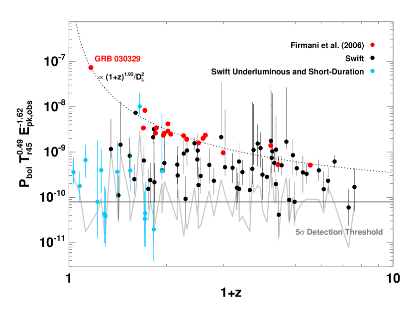
In Figure 9, we plot the observer-frame quantities used to form the Firmani et al. (2006) relation versus redshift. There is a moderately strong correlation in the Firmani et al. (2006) sample ($\tau_{K}=0.76$, $4.6\sigma$). Excluding the underluminous and short-duration Swift events as above, the Swift sample exhibits lower flux values, and the correlation among best-fit model parameters (Table 2) is weak ($\tau_{K}=0.17$, $1.9\sigma$). Because the Firmani et al. (2006) relation has a similar form to our detector threshold estimate (Section 2.4), as we describe below, the clustering in observer-frame quantities in Figure 9 is likely a consequence of a clustering above threshold (Figure 2; Top Left).

Additionally, it is plausible that the moderately strong correlation between these quantities and redshift in the pre-Swift sample arises from biases associated with optical transient detection. If the intrinsic optical flux tracks the $\gamma$-ray flux, then there will be a truncation below lines roughly parallel to the dotted line in Figure 9. We find that bright ($R<18$ mag) optical transients were not detected within 0.5 days of the GRB for 25% of events above $5\times 10^{-10}$ erg cm^-2 s^-0.51 keV^-1.62 in Figure 9. However, more than half of events below a line drawn at that value do not have bright optical counterparts. Pre-Swift host galaxy associations depended on tight localizations possible only from optical detections, whereas Swift-era host galaxies are often pin-pointed from XRT observations.

The redshift dependence of the observer frame quantities in the pre-Swift sample appears compelling in large part due to the presence of the bright GRB 0303029 (Figure 9) at low redshift. However, the Swift sample shows the high flux of this event to be anomalous. There are additional points — overlapping with the Swift cyan points in Figure 9 — which were discarded as outliers by Firmani et al. (2006).

If we re-write the Firmani et al. (2006) relation in terms of $n_{\rm bol}$, we find

$$n_{\rm bol,firmani}\approx 30\left\{{E_{\rm pk,obs}\over 100~{}{\rm keV}}\right\}^{0.62}T_{r45}^{-0.49}(1+z)^{-0.09}\\ \times\left\{{D_{L}(z=1)\over D_{L}}\right\}^{2}\left\{{1+z\over 2}\right\}^{2}\gamma~{}{\rm cm}^{-2}.$$ (19)

Equation 19 has a similar time dependence to our threshold. There is also a weak dependence on the burst $E_{\rm pk,obs}$. Ignoring the difference between $T_{90}$ and $T_{r45}$, the value of the threshold is in an order of magnitude lower than our estimated Swift threshold (Section 2.4). This is consistent with the relative fraction of expected hard/faint events in the Swift and pre-Swift samples determined in Section 4. The redshift variation in Equation 19 is extremely weak for $z\mathrel{\hbox{\hbox to0.0pt{\hbox{\lower 4.0pt\hbox{$\sim$}}\hss}\hbox{$>$}}}1$.

An explanation in terms of a threshold provides a natural explanation for why low-$z$ events like GRBs 051109B, 060218, 060614, and the short-duration GRBs do not fit on the Firmani et al. (2006) and other relations. In Sections 2.4 and 4.5, we discuss how these Swift short-duration and underluminous events, which are strong outliers to the $E_{\rm iso}$–$E_{\rm pk}$ relation, do follow the source frame correlation set by the detector threshold (Figure 2; Bottom Left).

A test of our claim that most pre-Swift high-energy correlations are due simply to the detector threshold is to also show that the pre-Swift underluminous and short duration events satisfy Equation (19). In terms of $E_{\rm iso}$, if the events are near threshold, the expected value is

$$E_{\rm iso,thresh}\approx 5\times 10^{49}\left\{{E_{\rm pk,obs}\over 100~{}{\rm keV}}\right\}^{1.62}\left\{{T_{r45}\over 5~{}{\rm s}}\right\}^{-0.49}\\ \times\left\{{D_{L}\over D_{L}(z=0.1)}\right\}^{2}\left\{{1.1\over 1+z}\right\}^{2}~{}{\rm erg}.$$ (20)

The observed $E_{\rm iso}$ and $E_{\rm obs,pk}$ for GRB 980425 at $z=0.0085$ (e.g., Kouveliotou et al., 2004; Ghirlanda, Ghisellini, & Lazzati, 2004) are $\approx 10^{48}$ erg and 120 keV, respectively. If we assume $T_{r45}=5$ s, then we find $E_{\rm iso,thresh}\approx 5\times 10^{47}$ erg. The observed $E_{\rm iso}$ and $E_{\rm obs,pk}$ for GRB 031203 at $z=0.105$ (e.g., Sazonov et al., 2004) are $\approx 5\times 10^{49}$ erg and $\mathrel{\hbox{\hbox to0.0pt{\hbox{\lower 4.0pt\hbox{$\sim$}}\hss}\hbox{$>$}}}190$ keV, respectively. If we assume $T_{r45}=5$ s, then we find $E_{\rm iso,thresh}\approx 5\times 10^{49}$ erg. The observed $E_{\rm iso}$ and $E_{\rm obs,pk}$ for short GRB 050709 at $z=0.16$ (e.g., Villasenor et al., 2005) are $\approx 10^{50}$ erg and 84 keV, respectively. If we assume $T_{r45}=0.5$ s, then we find $E_{\rm iso,thresh}\approx 10^{50}$ erg. This agreement is excellent.

Because we can understand the luminosities of these events in terms of a detector threshold, there is little reason to think of them as anomalously subluminous (see, e.g., Soderberg et al., 2004; Guetta et al., 2004; Watson et al., 2006a; Ghisellini et al., 2006). If our threshold versus redshift is in fact correct for short durations, then there is little reason to believe that the intrinsic energy release in short durations GRBs is different from that in long duration GRBs.

5. Conclusions

We fit for the durations and spectral parameters of 218 Swift GRBs, including 77 GRBs with redshifts. Unbiased estimates of $E_{\rm iso}$ and $E_{\rm pk,obs}$ (at least for $E_{\rm pk,obs}\mathrel{\hbox{\hbox to0.0pt{\hbox{\lower 4.0pt\hbox{$\sim$}}\hss}\hbox{$<$}}}1$ MeV) are possible for these events if we adopt a Bayesian spectral fitting approach, with relatively weak prior assumptions. Because $E_{\rm pk,obs}$ is typically poorly-constrained and correlates with $E_{\rm iso}$ in a complicated fashion, we rigorously propagate errors via a sampling of the posterior probability. We have searched for correlations among the observer frame quantities, and have found a family of correlations (Figure 2) which we argue to be due to the detector threshold. We have also measured apparently statistically significant correlations among host frame quantities (Sections 4.4 and 4.5).

Thanks to the large Swift BAT dataset, we now understand the probable origin of the $E_{\rm pk}$-$E_{\rm iso}$ correlation: a trigger threshold $\propto n_{\rm bol}$ and an intrinsic lack of bright relative to faint sources induces a strong observer-frame correlation between $E_{\rm pk,obs}$ and $S_{\rm bol}$. The apparent correlation strength is then amplified as we multiply both side of the equation by strong functions of redshift, in order to transform to the host frame quantities. The redshifts or fluence and $E_{\rm pk,obs}$ data can be drawn at random and do not have to correspond to the actual host galaxy redshifts or measured values in order to produce a significant correlation in the host frame quantities.

There are 3 strong and independent reasons to believe that the $E_{\rm pk}$-$E_{\rm iso}$ relation for both Swift and pre-Swift GRBs is an artifact of the detection threshold. First, a large fraction of the Swift GRB sample exhibits hard and underluminous spectra which are inconsistent with the pre-Swift relations, in agreement with indications from BATSE GRBs without redshifts. Second, the Swift GRB sample yields a powerlaw $E_{\rm pk}$-$E_{\rm iso}$ relation which is inconsistent at the $>5\sigma$ level with the pre-Swift relations, and with an intrinsic scatter at least a factor of 2 larger. Third, a dividing line between the pre-Swift and Swift samples can be plotted (Figure 8) using only the detector threshold, and the $E_{\rm pk}$-$E_{\rm iso}$ correlation significance can be shown to decrease dramatically if we correct for partial correlation with the probable shape of the threshold.

These faults appear to be shared by several other correlations among high-energy parameters reported in the literature (Section 4.5). It is likely that these contain largely redundant information which reduces to the shape of the detector threshold, at least for Swift BAT events. This insight also helps to explain why short-duration and underluminous events at low$-z$ appear to fall away from the relations (Section 4.6).

We stress that even if the relations contain information actually related to the physical properties of GRBs, the wide dispersion in the relations makes them useless as cosmology probes (see, also, Friedman & Bloom, 2005).

Nonetheless, it is still likely that the relations encapsulate important information about the intrinsic distribution of GRBs with luminosity. Extracting this information requires that we account accurately for the detector threshold. Turning this around, at the low energy end, the $E_{\rm pk}$-$E_{\rm iso}$ and other relations may be useful proxies for the detector threshold and other complicated biases (e.g., those associated with source localization, optical detection and redshift determination; Section 4.6). Accounting for these biases may be the most fruitful path toward uncovering true source frame relations in GRBs. This is clearly a critical step toward realizing the potential of Swift and future missions such as GLAST and EXIST.

Figure 1.— Time region definition, duration estimation, and spectral parameter estimation for example GRB 060105. (Top Panel) Light curve plotted with 1s binning. The automated algorithm finds four trigger regions over threshold and merges these into a burst window of width $\Delta t=87.4$s. This region is then extended backward by 0.46 s and forward by 3.22 s based on signal in the denoised light curve (overplotted in red) to define the final burst interval. (Middle Panel) The time-integrated spectrum is acceptably fit by a simple powerlaw (Table 2). (Bottom Panel) Using prior information (primarily on $E_{\rm pk,obs}$) we are able to infer the presence of a spectral break located well above the BAT detector bandpass, consistent with measurements by Konus-Wind (Golenetskii et al., 2006).

Figure 2.— Experimental determination of the BAT threshold in terms of $n_{\rm bol}/\sqrt{T_{90}}$. (Top Left) The histogram of 1–$10^{4}$ keV photon fluence $n_{\rm bol}$ (Table 2) divided by the square root of $T_{90}$ (Table 1) exhibits a narrow distribution and 90% of values are greater than a threshold of 3 ph cm^-2 s^-0.5. The red histogram shows the events with measured redshift. (Top Right) Scatter plot showing a correlation between $n_{\rm bol}$ and $T_{90}$ likely due to the threshold. The approximate threshold from the Top Left plot is also plotted. (Bottom Left) The trigger $S/N$ (Table 1) correlates tightly with $n_{\rm bol}/\sqrt{T_{90}}$. The best fit powerlaw (plotted) has index $\approx 1$ and normalization $S/N\approx 5$ at $n_{\rm bol}/\sqrt{T_{90}}=3$ ph cm^-2 s^-0.5. (Bottom Right) The effect of the threshold in the source frame versus redshift $z$.

Figure 3.— The role of the Bayesian priors over a large $E_{\rm pk,obs}$ range plotted versus best-fit powerlaw photon index $\alpha_{\rm best-fit}$. The dark black points and error bars show $E_{\rm pk,obs}$ determinations for events adequately fit by a powerlaw model (PLM). In the classical frequentist approach to spectral fitting, these spectra yield only limits (Table 2). Very large $E_{\rm pk,obs}$ values are extremeley uncommon, as is clear from the red points from BATSE (Kaneko et al., 2006), which are plotted using the GRBM high energy index $\alpha$ on the x-axis; we truncate the probability at high $E_{\rm pk,obs}$ through our model priors. We do not truncate the probability at low $E_{\rm pk,obs}$ until 1 keV, and it is clear that Swift measures $E_{\rm pk,obs}$ values (grey points) below the BATSE bandpass. A strong correlation between the best-fit photon index $\alpha_{\rm best-fit}$ for the black points — which is not necessarily $\alpha$ or $\beta$ in the GRBM due to the possible proximity of $E_{\rm pk,obs}$ to the bandpass — and $E_{\rm pk,obs}$ results (Section 3.5).

Figure 4.— Comparison of $E_{\rm pk,obs}$ and approximate bolometric fluences $S_{\rm bol}$ derived here to values reported in the GCN circulars for Konus-Wind (e.g., Golenetskii et al., 2006) or Suzaku (e.g., Hong et al., 2007) and the lines of equality. Although the BAT detector approaches zero effective area above 150 keV, we are able to accurately recover the true $E_{\rm pk,obs}$ and fluence without bias.

Figure 5.— Catalog values for the 1–$10^{4}$ keV photon ($n_{\rm bol}$) and energy ($S_{\rm bol}$) fluences and $\nu F_{\nu}$ spectral peak energy $E_{\rm pk,obs}$. (Top Left) Bayesian versus frequentist $E_{\rm pk,obs}$ estimates and the line of equality. The red arrows designate $E_{\rm pk,obs}^{\rm freq.}$ limits for the majority (66%) of BAT events. (Top Right) $E_{\rm pk,obs}$ versus the approximate bolometric fluence $S_{\rm bol}$. (Bottom Left) The approximately bolometric photon fluence scales as $S_{\rm bol}/E_{\rm pk,obs}$. (Bottom Right) The Swift sample contains an excess of low $E_{\rm pk,obs}$ events, similar to HETE-2 (Sakamoto et al., 2005), compared to the Kaneko et al. (2006) catalog of bright BATSE GRBs. In blue we plot the fit to the $E_{\rm pk,obs}$ (including errors) for each GRB (from Equations 16 and 17). We assume the red line as a prior in the fitting for each event in order to measure upper confidence interval bounds on $E_{\rm pk,obs}$. The histogram for Swift “short-duration” GRBs is given as a dashed histogram.

Figure 6.— Maximum posterior probability values for $E_{\rm pk}$ and $E_{\rm iso}$ (filled circles) for 77 Swift GRBs with measured redshifts (Table 2). Also plotted are samples from the 90% confidence region in $E_{\rm pk}$ and $E_{\rm iso}$ for each GRB (small gray dots). Outliers in terms of short burst duration or low-luminosity are labelled. The best fit lines from this study (excluding the underluminous and “short-duration” events) and from the Beppo-SAX sample of Amati et al. (2002) are also plotted. Events furthest from the Amati et al. (2002) line in terms of low $E_{\rm iso}$ and high $E_{\rm pk}$ are closer to detector thresholds (Figure 8).

Figure 7.— Posterior probability contours for a powerlaw relation $E_{\rm pk}=K~{}(E_{\rm iso}/[10^{52}{\rm~{}erg}])^{\eta}$ keV. We also plot ($K,\eta)$ for the sample divided into 3 redshift bins. Estimates of the relation before Swift and including early Swift data summarized in Amati et al. (2006) (and from Amati et al. (2002); Amati (2003); Ghirlanda, Ghisellini, & Lazzati (2004); Friedman & Bloom (2005); Nava et al. (2006)) are inconsistent with the current sample normalization $K$ at the $>5\sigma$ level. $E_{\rm pk}$ and $E_{\rm iso}$ values and confidence regions from Cabrera et al. (2007) for 28 of the events also used in this study are also fit (cyan point; Section 4.2). The marginal posterior distributions in $K$ and $\eta$ are plotted above the $X$ and to the right of $Y$ axes, respectively.

Figure 8.— $E_{\rm pk}$–$E_{\rm iso}$ truncation and the detector threshold. We can separate events consistent with the Amati et al. (2002) relation (black circles) from those inconsistent (red circles) by a line of constant $E^{0.5}_{\rm iso}/E_{\rm pk}$, which is approximately a line of constant $N_{\rm iso}/E_{\rm pk}$. The detection threshold scales as $N_{\rm iso}/\sqrt{T_{90}}$ (Section 2.4). For the units in the plot, because of convolution with the burst $T_{90}$ and $E_{\rm pk}$, the threshold is blurred and the observed instance is a jagged line. We also plot the median threshold. Hypothetical events below the purple line (which divides the red and black events and also touches the detection threshold at various points) are $\mathrel{\hbox{\hbox to0.0pt{\hbox{\lower 4.0pt\hbox{$\sim$}}\hss}\hbox{$>$}}}65$% more likely to be absent from pre-Swift catalogs.

Figure 9.— The observer frame quantities found to correlate tightly with redshift by Firmani et al. (2006) do not correlate tightly in the Swift sample. Both samples follow the same upper limit envelope. However, the Swift events extend to lower flux and stop at the detector threshold. Here, $P_{\rm bol}$ is the peak energy flux. The Swift threshold values (actual and median) are plotted, as is the best-fit line to the Firmani et al. (2006) sample. Error bars are not plotted for the (red) events considered in Firmani et al. (2006).

References

- Akritas & Siebert (1996) Akritas, M. G., & Siebert, J. 1996, A&A, 278, 919
- Amati (2003) Amati, L. 2003, ChJAA, 3 Suppl., 455
- Amati et al. (2002) Amati, L., et al. 2002, A&A, 390, 81
- Amati et al. (2006) Amati, L. 2006, MNRAS, 372, 233
- Arnaud (1996) Arnaud, K. A. 1996, Astronomical Data Analysis Software and Systems V, eds. Jacoby G. and Barnes J., ASP Conf. Series v101.
- Atteia (2003) Atteia, J.-L. 2003, A&A, 407, L1
- Band (2003) Band, D. L. 2003, ApJ, 588, 945
- Band et al. (1993) Band, D. L., et al. 1993, ApJ, 413, 281
- Band & Preece (2005) Band, D. L., & Preece, R. D. 2005, ApJ, 627, 319
- Barraud et al. (2003) Barraud, C., et al. 2003, A&A, 413, 281
- Barthelmy et al. (2005) Barthelmy, S. D., et al. 2005, Space Science Reviews, 120, 143
- Berger & Becker (2005) Berger, E., & Becker, G. 2005, GCN #3520
- Berger et al. (2005a) Berger, E., et al. 2005a, ApJ, 629, 328
- Berger et al. (2005b) Berger, E., et al. 2005b, ApJ, 634, 501
- Berger (2006) Berger, E. 2006, GCN #5962
- Berger & Gladders (2006) Berger, E., & Gladders, M. 2006, GCN #5170
- Berger et al. (2006a) Berger, E., et al. 2006a, GCN #4815
- Berger et al. (2006b) Berger, E., et al. 2006b, ApJ, 642, 979
- Berger (2007) Berger, E. 2007, ApJSubmitted, astro-ph/0702694
- Berger et al. (2007) Berger, E., et al. 2007, ApJaccepted, astro-ph/0611128
- Bloom et al. (2005) Bloom, J. S., et al. 2005, GCN #3758
- Bloom et al. (2006a) Bloom, J. S., et al. 2006a, GCN #5238
- Bloom et al. (2006b) Bloom, J. S., et al. 2006b, GCN #5217
- Bloom et al. (2006c) Bloom, J. S., et al. 2006c, GCN #5826
- Burrows et al. (2005) Burrows, D. N., et al. 2005, Space Science Reviews, 120, 165
- Butler (2007a) Butler, N. 2007a, ApJ, 656, 1001
- Butler (2007b) Butler, N. 2007b, AJ, 133, 1027
- Butler & Kocevski (2007a) Butler, N., & Kocevski, D. 2007a, astro-ph/0612564, ApJAccepted
- Butler & Kocevski (2007b) Butler, N., & Kocevski, D. 2007b, astro-ph/0702638, ApJAccepted
- Cabrera et al. (2007) Cabrera, J. I., et al. 2007, arXiv:0704.0791, MNRAS submitted
- Campana et al. (2006a) Campana, S., et al. 2006, Nature, 442, 1008
- Cash (1976) Cash, W. 1976, A&A, 52, 307
- Castro-Tirado et al. (2006) Castro-Tirado, A. J., et al. 2006, GCN #5218
- Cenko et al. (2006a) Cenko, S. B., et al. 2006a, GCN #4592
- Cenko et al. (2006b) Cenko, S. B., et al. 2006b, GCN #5155
- Cenko et al. (2007) Cenko, S. B., et al. 2007, GCN #6322
- Chen et al. (2005) Chen, H.-W., et al. 2005, ApJL, 634, L25
- Chen et al. (2007) Chen, H.-W., et al. 2007, GCN #6217
- Cucchiara et al. (2006a) Cucchiara, A., et al. 2006a, GCN #4729
- Cucchiara et al. (2006b) Cucchiara, A., et al. 2006b, GCN #5052
- Cucchiara et al. (2007) Cucchiara, A., et al. 2007, GCN #6083
- Curtis et al. (2007) Curtis, J. L., et al. 2007, in prep.
- D’Elia et al. (2005) D’Elia, V., et al. 2005, GCN #4044
- Della Valle et al. (2006) Della Valle, M., et al. 2006, Nature, 444, 1050
- Dupree et al. (2006) Dupree, A. K., et al. 2006, GCN #4969
- Fenimore & Ramirez-Ruiz (2000) Fenimore, E. E., & Ramirez-Ruiz, E., astro-ph/0004176
- Firmani et al. (2006) Firmani, C., et al. 2006, MNRAS, 370, 185
- Foley et al. (2005a) Foley, R. J., et al. 2005a, GCN #3483
- Foley et al. (2005b) Foley, R. J., et al. 2005b, GCN #4409
- Friedman & Bloom (2005) Friedman, A. S., & Bloom, J. S. 2005, ApJ, 627, 1
- Fugazza et al. (2005) Fugazza, D., et al. 2005, GCN #3948
- Fugazza et al. (2006) Fugazza, D., et al. 2006, GCN #5513
- Fynbo et al. (2005) Fynbo, J. P. U., et al. 2005, GCN #3749
- Fynbo et al. (2006a) Fynbo, J. P. U., et al. 2006a, A&A, 451, L47
- Fynbo et al. (2006b) Fynbo, J. P. U., et al. 2006b, GCN #5809
- Gehrels et al. (2004) Gehrels, N., et al. 2004, ApJ, 611, 1005
- Ghirlanda, Ghisellini, & Lazzati (2004) Ghirlanda, G., Ghisellini, G., & Lazzati D. 2004, ApJ, 616, 331
- Ghisellini et al. (2006) Ghisellini, G., et al. 2006, MNRAS, 372, 1699
- Golenetskii et al. (2006) Golenetskii, S., et al. 2006, GCN #4439
- Grazian et al. (2006) Grazian, A., et al. 2006, GCN #4545
- Gregory (2005) Gregory, P. 2005, Bayesian Logical Data Analysis for the Physical Sciences, Cambridge Uvinversity Press, Cambridge
- Guetta et al. (2004) Guetta, D., et al. 2004, ApJ, 615, 73
- Halpern & Mirabal (2005) Halpern, J. P., & Mirabal, N. 2005, GCN #5982
- Heise et al. (2000) Heise, J., et al. 2000, in Proc. 2nd Rome Workshop: Gamma-ray Bursts in the Afterglow Era, eds. E. Costa, F. Frontera, J. Hjorth (Berlin: Springer-Verlag), 16
- Hong et al. (2007) Hong, S., et al. 2007, GCN #6240
- Jakobsson et al. (2005) Jakobsson, P., et al. 2005, A&A, 447, 897
- Jakobsson et al. (2006a) Jakobsson, P., et al. 2006a, A&A, 460, L13
- Jakobsson et al. (2006b) Jakobsson, P., et al. 2006b, GCN #5298
- Jakobsson et al. (2006c) Jakobsson, P., et al. 2006c, GCN #5320
- Jakobsson et al. (2006d) Jakobsson, P., et al. 2006d, GCN #5617
- Jakobsson et al. (2006e) Jakobsson, P., et al. 2006e, GCN #5698
- Jakobsson et al. (2007a) Jakobsson, P., et al. 2007a, GCN #6283
- Jakobsson et al. (2007b) Jakobsson, P., et al. 2007b, GCN #6398
- Jaunsen et al. (2007a) Jaunsen, A. O., et al. 2007a, GCN #6010
- Jaunsen et al. (2007b) Jaunsen, A. O., et al. 2007b, GCN #6202
- Kaneko et al. (2006) Kaneko, Y., et al. 2006, ApJS, 166, 298
- Kawai et al. (2005) Kawai, N., et al. 2005, Nature, 440, 184
- Kelly (2007) Kelly, B. C. 2007, ApJAccepted, astro-ph/0705.2774
- Kippen et al. (2002) Kippen, R. M., et al. 2002, in Gamma-Ray Bursts and Afterglow Astronomy, ed. G. R. Ricker & R. Vanderspek (Melvill: AIP), 25
- Kocevski et al. (2007) Kocevski, D., et al. 2007, in prep
- Kolaczyk & Dixon (2000) Kolaczyk, E. D., Dixon, D. D. 2000, ApJ, 534, 490K
- Kouveliotou et al. (1993) Kouveliotou, C., et al. 1993, ApJ, 413, L101
- Kouveliotou et al. (2004) Kouveliotou, C., et al. 2004, ApJ, 608, 872
- Krimm et al. (2006) Krimm, H., et al. 2006, GCN #5704
- Lamb et al. (2004) Lamb, D. Q., et al. 2004, New A Rev., 48, 459
- Ledoux et al. (2006) Ledoux, C., et al. 2006, GCN #5237
- Ledoux et al. (2005) Ledoux, C., et al. 2005, GCN #3860
- Lee, Bloom, & Petrosian (2000) Lee, A., Bloom, E. D., & Petrosian, V. 2000, ApJS, 131, 21
- Li (2007) Li, L.-X. 2007, MNRAS Accepted, arXiv:0704.3128
- Liang & Zhang (2005) Liang, E., & Zhang, B. 2005, ApJ, 633, 611
- Lloyd, Petrosian, & Mallozzi (2000) Lloyd, N. M., Petrosian, V., & Mallozzi, R. S. 2000, ApJ534, 227
- Lupton (1993) Lupton, R. 1993, Statistics in Theory and Practice, Princeton University Press, Princeton
- Malesani et al. (2007) Malesani, D., et al. 2007, A&Asubmitted, arXiv
- Malmquist (1922) Malmquist, K. G. 1922, Lund Medd. Ser. I, 100, 1
- Melandri et al. (2006) Melandri, A., et al. 2006, GCN #4539
- Nakar & Piran (2005) Nakar, E., & Piran, T. 2005, MNRAS, 360, 73
- Nava et al. (2006) Nava, L., et al. 2006, preprint (astro-ph/0511499)
- Norris, Marani, & Bonnell (2000) Norris, J. P., Marani, G. F., & Bonnell J. T. 2000, ApJ, 534, 248
- Osip et al. (2006) Osip, D., et al. 2006, GCN #5715
- Paciesas et al. (1999) Paciesas, W. S., et al. 1999, ApJS, 122, 465
- Panaitescu (2007) Panaitescu, A. 2007, MNRAS submitted, arXiv/0705.1015
- Pellizza et al. (2006) Pellizza, L. J., et al. 2006, A&A, 459, L5
- Penprase et al. (2005) Penprase, B. E., et al. 2005, ApJ, 646, 358
- Perley et al. (2006) Perley, D. A., et al. 2006, GCN #5387
- Perley et al. (2007) Perley, D. A., et al. 2007, ApJsubmitted, astro-ph/0703538
- Pian et al. (2006) Pian, E., et al. 2006, Nature, 442, 1011
- Piranomonte et al. (2006a) Piranomonte, S., et al. 2006a, GCN #5626
- Piranomonte et al. (2006b) Piranomonte, S., et al. 2006b, GCN #4520
- Preece et al. (2000) Preece, R. D., et al. 2000, ApJ, 126, 19S
- Press et al. (1992) Press, W. H., et al. 1992, Numerical Recipes in C, (2nd ed.; Cambridge: Cambridge Univ. Press)
- Price et al. (2007) Price, P. A., et al. 2007, ApJL, 663, L57
- Prochaska et al. (2005) Prochaska, J. X., et al. 2005, GCN #3390
- Prochaska et al. (2006) Prochaska, J. X., et al. 2006, ApJ, 642, 989
- Protassov et al. (2002) Protassov, R., et al. 2002, ApJ, 571, 545
- Quimby et al. (2005) Quimby, R., et al. 2005, GCN #4221
- Reichart et al. (2001) Reichart, D. E., et al. 2001, ApJ, 552, 57
- Rol et al. (2006) Rol, E., et al. 2006, GCN #5555
- Romano et al. (2006b) Romano, P., et al. 2006a, A&A, 456, 917
- Ruiz-Velasco et al. (2007) Ruiz-Velasco, A. E., et al. 2007, ApJsubmitted, arXiv
- Sakamoto et al. (2004) Sakamoto, T., et al. 2004, ApJ, 602, 875
- Sakamoto et al. (2005) Sakamoto, T., et al. 2005, ApJ, 629, 311
- Sakamoto et al. (2006) Sakamoto, T., et al. 2006, HEAD Meeting Bulletin, 38, 380
- Sato et al. (2007) Sato, G., et al. 2007, ApJ, 657, 359
- Savaglio (2006) Savaglio, S., et al 2006, GCN #6166
- Sazonov et al. (2004) Sazonov, S. Y., et al. 2004, Nature, 430, 646
- Schady (2006) Schady, P., et al. 2006, GCN #5296
- Schaeffer (2003) Schaeffer, B. E. 2003, ApJ, 583, L67
- Schaeffer & Collazzi (2007) Schaeffer, B. E., & Collazzi, A. C. 2003, ApJL Accepted, astro-ph/07015481
- Soderberg et al. (2004) Soderberg, A. M., et al.2004, Nature, 430, 648
- Soderberg et al. (2005) Soderberg, A. M., et al. 2005, GCN #4186
- Soderberg et al. (2006) Soderberg, A. M., et al. 2006, ApJ, 650, 261
- Soderberg et al. (2007) Soderberg, A. M., et al. 2007, ApJ, 661, 982
- Sollerman et al. (2007) Sollerman, J., et al. 2007, A&A, 466, 839
- Thöne et al. (2006a) Thöne, C. C., et al. 2006a, GCN #5373
- Thöne et al. (2006b) Thöne, C. C., et al. 2006b, GCN #5812
- Thöne et al. (2007) Thöne, C. C., et al. 2007, GCN #6379
- Villasenor et al. (2005) Villasenor, J. S., et al. 2005, Nature, 437, 855
- Vreeswijk et al. (2006) Vreeswijk, P., et al. 2006, GCN #5535
- Watson et al. (2006a) Watson, D., et al. 2006a, ApJ, 636, 967
- Watson et al. (2006b) Watson, D., et al. 2006b, ApJ, 652, 1011
- Willingale et al. (2007) Willingale, R., et al. 2007, astro-ph/0612031
- Yonetoku et al. (2004) Yonetoku, D., et al. 2004, ApJ, 609, 935