Are all highly liquid securities within the same class?

Abstract

In this manuscript we analyse the leading statistical properties of fluctuations of ($\log$) $3$-month US Treasury bill quotation in the secondary market, namely: probability density function, autocorrelation, absolute values autocorrelation, and absolute values persistency. We verify that this financial instrument, in spite of its high liquidity, shows very peculiar properties. Particularly, we verify that $\log$-fluctuations belong to the Lévy class of stochastic variables.

Financial markets have become a paradigmatic example of complexity and the focus of plenty of work within physics. Specifically, several techniques, mainly related to statistical physics (e.g., stochastic dynamics, theory of critical phenomena or nonlinear systems), have been applied either to reproduce or simply verify several properties, e.g., the probability density functional form (PDF), or the autocorrelation function (ACF) of financial observables books ; book2 ; book3 . The systematic (asymptotic) power-law behaviour found for quantities such as price/index fluctuations, or traded volume has been pointed out to be at the helm of the multifractal character of financial time series mandelbrot-fractals-scaling , a feature that is also regular in out-of-equilibrium systems amit . On the account of the background on this type of phenomena, in which scale invariance also rules, it has come out the endeavour to identify universality classes for financial markets defined by the exponents that characterise their main statistical properties. Explicitly, these classes indicate the existence of a common behaviour for systems within the same class apart their microscopic or specific details stanley-colloqium . On this way, it has been suggested stanley-colloqium that financial products like securities with a very high level of liquidity (high trading activity) might present similar characteristics. As an example, it has been shown that, despite of the fact that in their essence stocks and commodities are completely different financial instruments (securities), their (daily) price fluctuations behave on a very similar way, i.e., they can be enclosed in the same class matia-amaral-bp .

Within securities are also public debt bonds like United States (US) Treasury bills debt ; bali . The US Treasury bills (T-bills) are marketable bonds issued by the US federal government and represent one of the debt financing instruments used by the Treasury Department t-bill . T-bills are classified as zero-coupon bonds that are sold in the primary market at a discount of the face value in order to present a positive yield to maturity which can be $28$ ($1$ month), $91$ ($3$ months), or $182$ ($6$ months) days. In regard of this, they are considered to be the most risk-free investment in the USA. This makes of T-bills an important and heavily traded (i.e., highly liquid) financial instrument in the secondary market where they are quoted on an annual percentage yield to maturity.

In the sequel of this manuscript we study some of the main statistical features of the $3$-month US T-bills traded on the secondary market. Our time series, $\left\{Q_{t}\right\}$, which is named $DTB3$ by the Federal Reserve, is composed by $3$-month US T-bill daily prices and runs from the $4^{th}$ January $1954$ up to the $26^{th}$ February $2007$ in a total of $13866$ trading days data-url . Our choice for a maturity of $3$ months is justified by the fact that it is the most used interest rate maturity in derivative financial products like call-put options. To compare the statistical properties of $DTB3$ daily $\log$-value fluctuations, $\tilde{r}_{t}=\ln Q_{t}-\ln Q_{t-1}$, we use the daily $\log$-index fluctuations, $\tilde{r}_{t}^{\prime}=\ln S_{t}-\ln S_{t-1}$, of $SP500$ time series, $\left\{S_{t}\right\}$, which runs the same time interval as $DTB3$. Both fluctuation time series, $\left\{\tilde{r}_{t}\right\}$ and $\left\{\tilde{r}_{t}^{\prime}\right\}$ have been subtracted of respective averages, $\left\langle\tilde{r}_{t}^{(\prime)}\right\rangle$, and normalised by standard deviation $\sigma_{\tilde{r}^{(\prime)}}$, i.e., $r_{t}^{(\prime)}=\left[\tilde{r}_{t}^{(\prime)}-\left\langle\tilde{r}_{t}^{(\prime)}\right\rangle\right]/\sigma_{\tilde{r}^{(\prime)}}$. (from here on the prime stands for $SP500$ quantities, and $x$ is used in definitions to represent any observable upon analysis).

Moving ahead, we shall now analyse and compare primary and more usually studied statistical features. Commencing with the analysis of ACF,

$$C_{x}\left(\tau\right)=\frac{\left\langle x_{t}\,x_{t+\tau}\right\rangle-\left\langle x_{t}\,\right\rangle^{2}}{\left\langle x_{t}^{2}\,\right\rangle-\left\langle x_{t}\,\right\rangle^{2}},$$ (1)

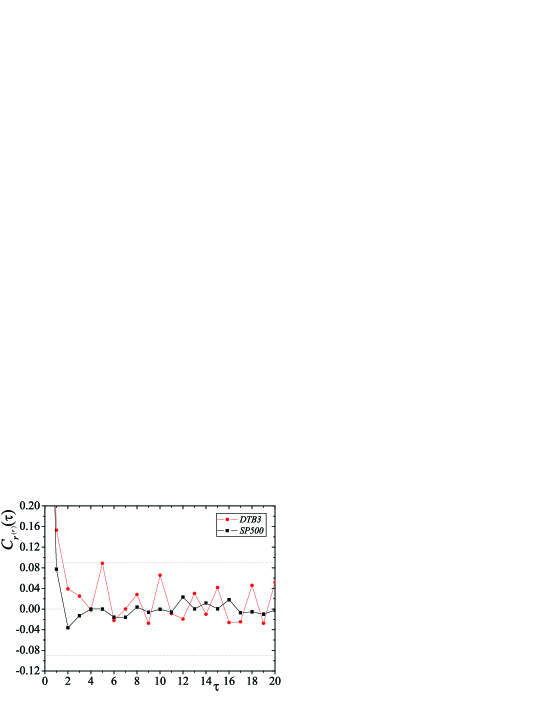
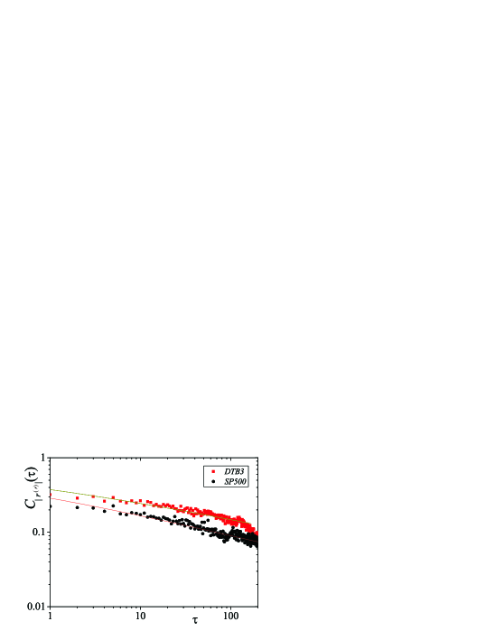
we have verified a noteworthy difference between $\left\{r_{t}\right\}$ and $\left\{r_{t}^{\prime}\right\}$. Firstly, as depicted in Fig. 1, $C_{r}\left(1\right)$ clearly exceeds three time noise level within which typical interday correlation values of $SP500$ and other indices as well books lay in. Additionally, correlation values greater than noise level have been measured at least for lag $\tau=5,10$ days. We attribute the origin of this feature to the fact that T-bills are weekly ($5$ trading days) sold at the primary market. Concerning the ACF of absolute values, we have not observed any relevant differences. Both curves are fairly described by (asymptotic power-law) $q_{c}^{(\prime)}$-exponential functions,

$$C_{\left|r^{(\prime)}\right|}\left(\tau\right)=\,\left[1-\left(1-q_{c}^{(\prime)}\right)\,\mathcal{T}^{(\prime)}\mathcal{\,}\tau^{2}\right]^{\frac{1}{1-q_{c}^{(\prime)}}},$$ (2)

where $q_{c}^{(\prime)}$ gives the decaying exponent, and $\mathcal{T}^{(\prime)}$ characteristic parameter. The value $q_{c}=4.7\pm 0.1$ is not far from $q_{c}^{\prime}=4.3\pm 0.1$, and both are in accordance with previous values obtained for $SP500$ amaral-cps-pre or $DJIA$ equities smdq-canberra . For $\mathcal{T}^{(\prime)}$ we have obtained $\mathcal{T}=0.45\pm 0.05$, and $\mathcal{T}^{\prime}=0.77\pm 0.05$.

Figure 1: (colour on-line) Autocorrelation function Eq. 1, $C\left(\tau\right)$ vs. $\tau$ of $r_{t}^{(\prime)}$ (left panel) and $\left|r_{t}^{(\prime)}\right|$ in a $\log$-$\log$ scale (right panel). It is visible that $r_{t}$ is correlated for immediate correlations and presents measurable correlations every multiple of $5$ days lag. The autocorrelation of $\left|r_{t}^{(\prime)}\right|$ can be described by Eq. (2) with $q_{c}=4.7\pm 0.1$, $\mathcal{T}=0.45\pm 0.05$ ($\chi^{2}/n=2\times 10^{-4}$, $R^{2}=0.9$) for $DTB3$, and $q_{c}^{\prime}=4.3\pm 0.1$, $\mathcal{T}^{\prime}=0.77\pm 0.05$ ($\chi^{2}/n=10^{-4}$, $R^{2}=0.9$) for $SP500$. The dashed line in left panel represents three times the noise level bounds.

Stronger dissimilarity has appeared on the PDFs, which we have fitted for $q$-Gaussian distributions,

$$\mathcal{G}_{q}\left(x\right)=\mathcal{A}\,\left[1-\left(1-q\right)\,\mathcal{B\,}x^{2}\right]^{\frac{1}{1-q}},\qquad\left(q<3\right),$$ (3)

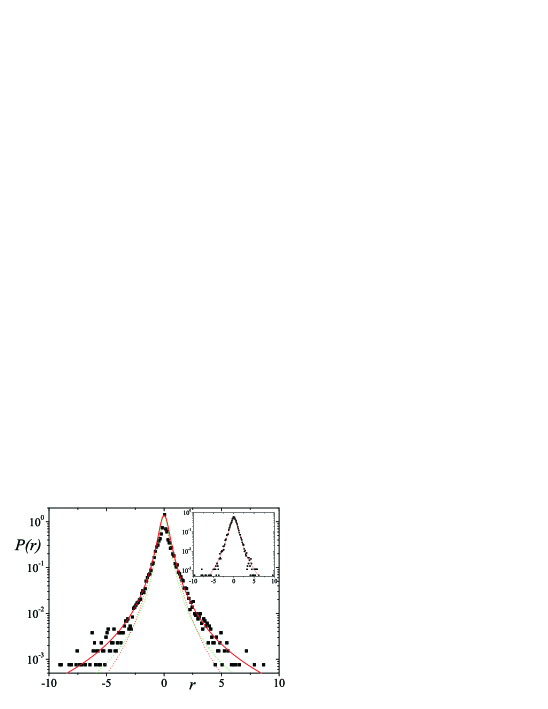
where $\mathcal{A}$ is the normalisation, and $\mathcal{B}$ is related to the “width” of the distribution determined by its $q$-generalised second order moment, $\sigma_{q}^{\,2}=\int x^{2}\ \left[P\left(x\right)\right]^{q}\ dx/\int\left[P\left(x\right)\right]^{q}dx$, in the form, $\mathcal{B}=\left[\sigma_{q}^{\,2}\left(3\,q-1\right)\right]^{-1}$ tsallis-milan . When $q<5/3$, standard deviation is finite and the equality $\mathcal{B}=\left[\sigma^{2}\left(5-3\,q\right)\right]^{-1}$ is also valid. For $q<3$, Distribution (3) emerges from optimising non-additive (Tsallis) entropy upon appropriate constraints ct . In the limit $q\rightarrow 1$ the Gaussian distribution is obtained, $\mathcal{G}_{1}\left(x\right)\equiv\mathcal{G}\left(x\right)$. Regardless both of the two fluctuations are well described by Eq. (3), the values of $q$ are qualitatively quite different. Namely, we have obtained the best fit for $q=1.72\pm 0.02$ for $DTB3$, and $q^{\prime}=1.49\pm 0.01$ for $SP500$ (see Fig. 2) . The latter is in accordance with prior analysis books ; book2 ; book3 ; amaral-cps-pre ; q-arch . Such a disparity has clear implications on the attractor in probability space of each observable when we consider the addition of fluctuations defining variable $R_{N,\,t}^{(\prime)}\equiv\sum_{i=0}^{N-1}r_{t+i}^{(\prime)}$. Since the two signals are essentially uncorrelated, in the sense that ACF rapidly attains at noise level, standard central limit theorems do apply araujo . In other words, for $SP500$, by reason of its entropic index $q$ is smaller than $\frac{5}{3}$, $\sigma^{\prime}$ is finite, hence the convolution of PDF $\log$-$SP500$ fluctuations leads to the Gaussian distribution, $\mathcal{G}\left(R_{N}^{\prime}\right)=\frac{1}{\sqrt{2\,\pi\,N\,\left(\sigma^{\prime}\right)^{2}}}\exp\left[-\frac{R_{N}^{\prime}}{2\,N\,\left(\sigma^{\prime}\right)^{2}}\right]$ (for $N\rightarrow\infty$, and since the daily time series has been normalised upon a finite series, $\sigma^{\prime}\approx 1$). Conversely, the entropic index for $DTB3$ is greater than $\frac{5}{3}$, which makes $\sigma$ actually incommensurable. Thus, according to the Lévy-Gnedenko central limit theorem araujo , the attracting distribution (for $N\rightarrow\infty$) is an $\alpha$-stable distribution,

$$\mathcal{L}_{\alpha}\left(R_{N}\right)=\frac{1}{2\,\pi}\int_{-\infty}^{+\infty}\exp\left[-i\,k\,R_{N}-a\left|k\right|^{\alpha}\right]dk,$$ (4)

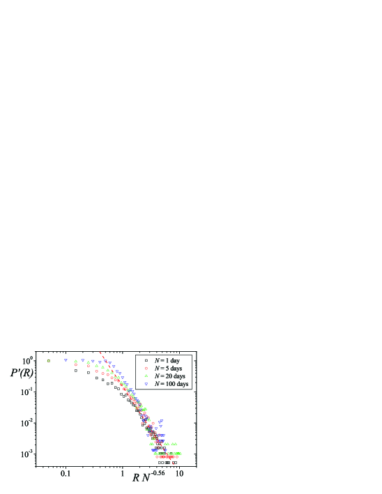
with $\alpha=\left(3-q\right)/\left(q-1\right)$, which follows, for large $N$, the scaling law $\mathcal{L}_{\alpha}\left(R_{N}\right)=N^{-1/\alpha}\mathcal{L}_{\alpha}\left(\frac{R_{N}}{N^{1/\alpha}}\right)$, and $\mathcal{L}_{\alpha}\left(R_{N}\right)\sim R_{N}^{-\alpha-1}$. As it is visible in Fig. 2, the PDFs of properly scaled $R_{N}$ variables obtained from $r\left(t\right)$ signal asymptotically collapse exhibiting a tail described by $\alpha\approx 1.77$, as it happens for variables whose attractor is a $\alpha$-stable distribution (see Ref. catania ). This constitutes, in our point of view, a substantial difference between $3$-month T-bill daily fluctuations and other financial fluctuations, by the fact that it represents a drastic change of the attractor.

Figure 2: (colour on-line) Left panel: PDF, $P\left(r\right)$ vs. $r$ in $\log$-linear scale. Symbols are obtained from data and the full line represents the best numerical adjustment for Eq. (3), with $q=1.72\pm 0.02$ and $\mathcal{B}=5.9\pm 0.4$ ($R^{2}=0.96$ and $\chi^{2}/n=3\times 10^{-3}$). The dotted line is the best fit for $\mathcal{G}_{q}\left(r\right)$, but imposing $q=q^{\prime}=1.49$ as in $SP500$ case shown at the in-set ($\mathcal{B}^{\prime}=2.23\pm 0.09$, $R^{2}=0.99$, and $\chi^{2}/n=3\times 10^{-4}$ ). The dashed line represents the best fit with $q=1.666$ ($\mathcal{B}=8.2\pm 0.6$) (on the edge of finite variance). Right panel: $P^{\prime}\left(R_{N}\right)=\frac{P\left(R_{N}\right)}{P\left(0\right)}N^{1/\alpha.}$ vs. $R_{N}\,N^{-1/\alpha}$ for $N=1$, $5$, $20$, $100$ days in $\log$-$\log$ scale. The asymptotic collapse of the curves, described by a tail exponent of $1+\alpha=2\frac{1}{q-1}=2.77$ is visible.

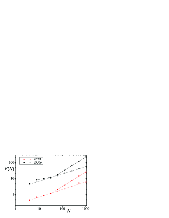
Within a macroscopic framework, the long-lasting form of the absolute price fluctuations ACF has been held responsible for the non-Gaussian behaviour of financial securities fluctuations long-volatility ; smdq-qf . To further analyse the persistency of absolute fluctuations, we have applied the $DFA$ method to assess the Hurst exponent, $H$, of $\left|r_{t}^{(\prime)}\right|$ time series and shuffled $\left\{\left|r_{t}^{(\prime)}\right|\right\}$ (procedure presented in dfa ). The results are exhibited in Fig. 3, where $N$ represents the lenght of the time series dfa . For $N>40$ we have verified that $DTB3$ presents a strong persistent behaviour as $SP500$ does with $H=0.90\pm 0.02$ and $H^{\prime}=0.90\pm 0.03$. For $N<40$ we verify a crossover, but this time index and T-bill fall apart with $H=0.50\pm 0.02$ (like a Brownian motion) and a specious $H^{\prime}=0.27$ (antipersistency). It is known that the presence of spikes and locality on persistency might introduce spurious features on DFA analysis dfa-bad ; dfa-bad1 ; dimatteo of persistent signals leading to $H<1/2\$values for small $N$. We attribute to this fact the emergence of $H\leq 1/2$ values.

Figure 3: (colour on-line) Left panel: Root-mean-square deviation $F\left(N\right)$ vs. $N$ for integrated absolute fluctuations time series of $DTB3$ (squares), and $SP500$ (circles). The full symbols are from the ordered series and empty symbols from shuffled signals. For large $N$ we have measured a Hurst exponent of $0.90\pm 0.02$ ($DTB3$), and $0.90\pm 0.03$ ($SP500$). For small $N$, T-bills absolute fluctuations $\log$-fluctuations presents a behaviour similar to white noise while $SP500$ exhibits a antipersistent behaviour.

Another property we have analysed are the correlations between fluctuations and absolute fluctuations bouchaud-leverage ,

$$L\left(\tau\right)=\frac{\left\langle r_{t}^{(\prime)}\,\left[r_{t+\tau}^{(\prime)}\right]^{2}\right\rangle}{\left\langle\left[r_{t+\tau}^{(\prime)}\right]^{2}\right\rangle^{2}}.$$ (5)

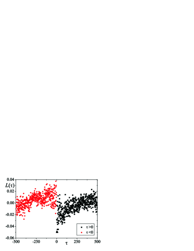
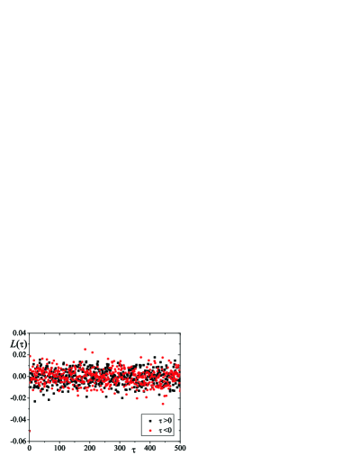
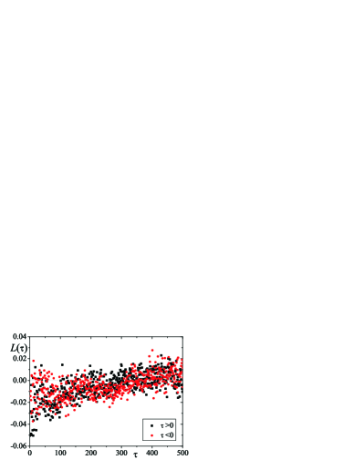
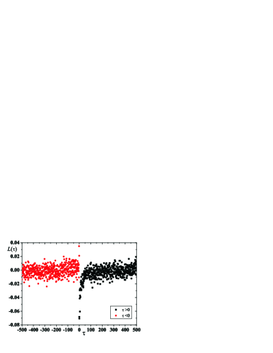
It has been verified in several securities and financial indices that $L\left(\tau\right)=0$ for $\tau<0$, and $L\left(\tau\right)\sim-\exp\left[-\tau/\lambda\right]$ for $\tau\geq 0$. This behaviour, known has leverage effect leverage , is intimately related to risk-aversion and negative skew of price fluctuations PDF. In defiance of the noisy $L\left(\tau\right)$ which has inhibited us to present a trusty quantitative description, it is plausible to affirm that $DTB3$ fluctuations also show time symmetry breaking, but in an antisymmetrical fashion, $L\left(-\tau\right)=-L\left(\tau\right)$, as it is understandable from Fig. 4. For $\tau<0$, there is a positive correlation between fluctuations and future absolute fluctuations, whereas for $\tau>0$, there exists a negative correlation between fluctuations and future absolute fluctuations. This antisymmetric behaviour has clear implications on dynamical mimicking. As an example, the Heston approach to financial fluctuations heston ; yakovenko , in which the noises of stochastic equations for the fluctuation and instantaneous variance are anti-correlated, must be modified in order embrace our empirical observations of T-bill $\log$-fluctuations.

Figure 4: (colour on-line) $L\left(\tau\right)$ vs. $\tau$ of $DTB3$ (left), and shuffled $\left\{r_{t}\right\}$ (centre left). Comparing both panels and taking into account noise level (dashed lines) it is visible the existence of a functional form for $L\left(\tau\right)$. Centre right panel: $L\left(\tau\right)$ for $\tau>0$ and $-L\left(-\tau\right)$ for $\tau<0$ vs. $\tau$. At right panel, $L\left(\tau\right)$ vs. $\tau$ of $SP500$ for mere illustration purposes.

To summarise, in this manuscript we have analysed a set of statistical properties of daily fluctuations of the $3$-month T-bill trading value, a highly liquid security. Our results have shown important differences between this financial instrument and a paradigmatic example of financial securities statistical properties, the daily fluctuations of $SP500$ index which also presents similar properties to other debt bonds books . Specifically, we have verified that T-bill daily fluctuations PDF belong to the $\alpha$-stable class of distributions, while other liquid securities that have been studied so far present the Gaussian distribution as the attractor in PDF space. This represents a fundamental justification for the well-known difficulties on the construction (namely specification) and implementation (namely identification and estimation) of generalised spot interest rate models t-bill-problems , which are always built assuming a finite standard deviation, unlike Lévy-Gnedenko class of random variables. Moreover, we have unveiled that the fluctuations-fluctuations magnitude correlation function presents an antisymmetric form, i.e., a different behaviour than the “leverage effect” that has been verified in other securities.

Our results emphasise the idea that liquidity is not the only factor to take into account when we aim to define a behavioural class for financial securities matia-amaral-bp ; eisler-kertesz-scaling . Properties such as the nature of the financial instrument under trading are actually relevant for its dynamics and categorisation. We address to future work the development of dynamical scenarios capable of reproducing the statistical properties we have presented herein.

SMDQ acknowledges C. Tsallis for several discussions on central limit theorems, L. Borland for practical aspects of financial trading, R. Rebonato for bibliographic references, and two anonymous colleagues for their comments that boosted the contents of this manuscript. The work presented benefited from infrastructural support from PRONEX/MCT (Brazilian agency) and financial support from FCT/MCES (Portuguese agency).

References

- (1) J.-P. Bouchaud and M. Potters, Theory of Financial Risks: From Statistical Physics to Risk Management (Cambridge University Press, Cambridge, 2000)
- (2) R.N. Mantegna and H.E. Stanley, An introduction to Econophysics: Correlations and Complexity in Finance (Cambridge University Press, Cambrigde, 1999)
- (3) J. Voit, The Statistical Mechanics of Financial Markets (Springer-Verlag, Berlin, 2003).
- (4) B.B. Mandelbrot, Fractals and Scaling in Finance (Springer, New York, 1997).
- (5) D. J. Amit, Field theory, the renormalization groups, and critical phenomena (World Scientific, Singapore, ).
- (6) H.E. Stanley, L.A.N. Amaral, S.V. Buldyrev, P. Gopikrishnan, V. Plerou, and M.A. Salinger, Proc. Nat. Acad. Sci. USA 99, 2561 (2002).
- (7) K. Matia, L.A.N. Amaral, S. Goodwin, and H.E. Stanley, Phys. Rev. E 66, 045103 (2002).
- (8) R. Rebonato and V. Gaspari, Quant. Finance 6, 297 (2006).
- (9) T. G. Bali, Ann. Oper. Res. 151, 151 (2007)
- (10) http://www.treasurydirect.gov/indiv/products/products.htm
-
(11)
Data available at URL:
http://research.stlouisfed.org/fred2/ - (12) P. Gopikrishnan, V. Plerou, L.A.N. Amaral, M. Meyer, and H.E. Stanley, Phys. Rev. E 60, 5305 (1999).
- (13) S.M.D. Queirós, L.G. Moyano, J. de Souza, and C. Tsallis, Eur. Phys. J. B 55, 161 (2007).
- (14) C. Tsallis, Milan J. Math. 73, 145 (2005).
- (15) C. Tsallis, J. Stat. Phys. 52, 479 (1988); C. Tsallis, R.S. Mendes, and A.R. Plastino, Physica A 261, 534 (1998).
- (16) S. M. Duarte Queirós, arXiv:0705.3248 (preprint, 2007).
- (17) A. Araujo and E. Guiné, The Central Limit Theorem for Real and Banach Valued Random Variables (John Wiley & Sons, New York, 1980).
- (18) C. Tsallis and S.M. Duarte Queirós, to appear in Proc. Int. Conf. on Complexity, Metastability and Nonextensivity, Catania, 2007, S. Abe, H.J. Herrmann, P. Quarati, A. Rapisarda, and C. Tsallis (eds.) (AIP, 2008). arXiv:0709.4656 (preprint, 2007).
- (19) M. Potters, R. Cont, and J.P. Bouchaud, Europhys. Lett. 41, 239 (1998).
- (20) S.M. Duarte Queirós, Quant. Financ. 5, 475 (2005).
- (21) C.-K. Peng , S.V. Buldyrev, S. Havlin, M. Simons, H.E. Stanley, and A.L. Goldberger, Phys. Rev. E 49 (1994) 1685.
- (22) Z. Chen, P.Ch. Ivanov, K. Hu, and H.E. Stanley, Phys. Rev. E 65, 041107 (2002).
- (23) Z. Chen, K.Hu, P.Carpena, P. Bernaola-Galvan, H.E. Stanley, and P.Ch. Ivanov, Phys. Rev. E 71, 011104 (2005).
- (24) M. Bartolozzi, C. Mellen, T. Di Matteo, and T. Aste, Eur. Phys. J. B 58, 207 (2007).
- (25) J.P. Bouchaud, A. Matacz, and M. Potters, Phys. Rev. Lett. 87, 228701 (2001).
- (26) J.C. Cox and S.A. Ross, J. Fin. Eco. 3, 145 (1976).
- (27) S.L. Heston, Rev. Fin. Stud. 6, 327 (1993).
- (28) A.A. Dragulescu, V.M. Yakovenko, Quant. Finance 2, 443 (2002).
- (29) G.J. Jiang, J. Fin. Quant. An. 33, 465 (1998) and references therein.
- (30) Z. Eisler and J. Kertész, Europhys. Lett. 77, 28001 (2007).